Curvature perturbation spectra from waterfall transition, black hole constraints and non-Gaussianity

Abstract

We carried out numerical calculations of a contribution of the waterfall field to the primordial curvature perturbation (on uniform density hypersurfaces) $\zeta$, which is produced during waterfall transition in hybrid inflation scenario. The calculation is performed for a broad interval of values of the model parameters. We show that there is a strong growth of amplitudes of the curvature perturbation spectrum in the limit when the bare mass-squared of the waterfall field becomes comparable with the square of Hubble parameter. We show that in this limit the primordial black hole constraints on the curvature perturbations must be taken into account. It is shown that, in the same limit, peak values of the curvature perturbation spectra are far beyond horizon, and the spectra are strongly non-Gaussian.

1 Introduction

In last two years an interest in hybrid inflation models was very much revived [1, 2, 3, 4, 5, 6, 7, 8] (see also earlier works [9, 10]). The main questions which were discussed are dynamics of the waterfall field and its influence on the total spectrum of density perturbations produced by inflationary expansion. It was suggested, in particular, that fluctuations in the waterfall field could lead to non-Gaussian curvature perturbation at rather large scales (even, possibly, at cosmological scales). Note that, in general, hybrid inflation models remain theoretically attractive up to now, especially in the context of supergravity and string theories (see, e.g., [11, 12]).

In many cosmological scenarios the period just after the end of inflation, i.e., the inflaton decay and the subsequent evolution of the decay products to a thermal equilibrium starts with preheating [13, 14, 16, 15]. One of the most studied models is hybrid inflation with tachyonic preheating. It had been shown in [17] that preheating after hybrid inflation goes through the tachyonic amplification due to the dynamical symmetry breaking, when one of the fields rolls to the minimum through the region where its effective mass-squared is negative. In the process of this rolling amplitudes of field fluctuations grow exponentially leading to a fast decrease of a height of the inflationary potential (“false vacuum decay”).

As is shown in the recent papers [1, 2, 3, 4, 6, 7, 8] the power spectrum of the comoving curvature perturbations from the waterfall field in hybrid inflation with tachyonic preheating is very blue: it depends on comoving wavenumber $k$ like $(k/k_{*})^{3}$ (for $k<k_{*}$) and is negligible on the cosmological scales. Absolute value of the spectrum amplitude at $k\sim k_{*}$ (as well as the value of $k_{*}$) depends on model parameters. In principle, this spectrum at $k\sim k_{*}$ may be quite substantial, and, in this case, it may be constrained by data of primordial black hole (PBH) and relict gravitational wave (GW) searches.

The amplification of curvature perturbations after preheating (e.g., in two-field inflation models) and blue spectra of the curvature perturbations on the constant energy density hypersurfaces, $\zeta$, behaving like $\sim k^{3}$ on super-horizon scales (in a case of the quadratic inflationary potential) had been predicted in many works (see, e.g., [18, 19, 20]). Another example where the steeply blue ($\sim k^{3}$) curvature perturbation spectrum is predicted is one of models of false vacuum inflation, in which the inflationary potential has a local minimum for a trapping of the field and a high temperature correction for a termination of inflation [21, 22].

In more recent studies of preheating processes [23, 24, 25, 26], primordial density perturbation spectra with blue tilt or, more generally, spectra having broad peak features at some $k_{*}$ value are predicted in two-field models of inflation ending by preheating (going through the parametric resonance) [23] and even in one-field inflation models (in particular, in models with tachyonic preheating after small-field inflation [24, 25]). The characteristic values of $k_{*}$ (i.e., the $k$-values of modes which become dominant as a result of tachyonic amplification or parametric resonance) are different in different models. In preheating after chaotic inflation [16, 27] where the perturbations are amplified by parametric resonance, power spectra are peaked at scales $k/aH\gg 1$, whereas in models of small-field inflation the spectra may be peaked around the Hubble scale. In preheating after hybrid inflation, the typical scale of $k$-values amplified by the tachyonic instability must be sub-Hubble if the phase transition is fast, i.e., if it takes less than a Hubble time [1, 26]. Clearly, the $k$-value of the dominantly amplified mode is an important characteristic of a preheating model because large curvature and density perturbations of the Hubble size may result in an abundant production of PBHs and GWs.

In the first stage of tachyonic preheating in models of hybrid inflation the amplification of initial quantum fluctuations of the non-inflaton field is realized due to the classical inflaton rolling or, in a case of the small initial velocity of the inflaton field, due to processes of quantum diffusion [17]. The former case is characterized by the existence of a period of the linear evolution of the non-inflaton field. The evolution in this case can be studied using the cosmological perturbation theory [28, 29, 30] or $\delta N$ approach [31, 32, 33, 34].

In the present paper we want to study in detail the dependence of the primordial curvature perturbations produced by hybrid inflation with tachyonic preheating on parameters of the inflationary potential. We show, in particular, that perturbation amplitudes strongly depend on the mass of the waterfall field $m_{\chi}$. More exactly, it depends on the relation $|m_{\chi}^{2}/H^{2}|$, where $H$ is a value of the Hubble parameter during inflation. At small values of this relation, $|m_{\chi}^{2}/H^{2}|\sim 1$, the waterfall transition is rather slow, and the expansion of the Universe can not be ignored. Our main aim is to predict concrete values of the perturbation spectrum amplitudes, as well as a form of the $k$-dependence of the spectrum. So, we preferred to use the results of the numerical (rather than analytical) solution of the equations for the time evolution of the waterfall field. The approximate analytic expression for the power spectrum amplitude, according to which one has, roughly, [8]

$${\cal P}_{\zeta}\sim\left|\frac{H^{2}}{m_{\chi}^{2}}\right|\cdot\left(\frac{k}{k_{*}}\right)^{3},\;\;\;\;\;k<k_{*},$$ (1.1)

was obtained in the limit of the fast waterfall transition, when $|m_{\chi}^{2}|\gg H^{2}$, and can not be a priori used in a whole region of the parameter space. This formula works well when number of e-folds of cosmological expansion during waterfall is not too small (say, $N\gtrsim 0.1$). If $N\ll 0.1$, eq. (1.1) must be multiplied on the factor which is proportional to $N$ and can be much less than $1$ [8].

The plan of the paper is as follows. In section 2 we calculate the time evolution of the power spectra of the waterfall field perturbations and the spectra at the end of the waterfall. The curvature perturbation spectra from the waterfall, as a function of model parameters, are calculated in section 3. In section 4 we give estimates for the possibility of PBH production in hybrid inflation model, with taking into account the non-Gaussianity of produced perturbations. Section 5 contains our conclusions.

2 Calculation of waterfall field amplitudes

We consider the hybrid inflation model which describes an evolution of the slowly rolling inflaton field $\phi$ and the waterfall field $\chi$, with the potential [35, 36]

$$V(\phi,\chi)=\left(M^{2}-\frac{\sqrt{\lambda}}{2}\chi^{2}\right)^{2}+\frac{1}{2}m^{2}\phi^{2}+\frac{1}{2}\gamma\phi^{2}\chi^{2}.$$ (2.1)

The first term in eq. (2.1) is a potential for the waterfall field $\chi$ with the false vacuum at $\chi=0$ and true vacuum at $\chi_{0}^{2}=2M^{2}/\sqrt{\lambda}\equiv v^{2}$. The effective mass of the waterfall field in the false vacuum state is given by

$$m_{\chi}^{2}(\phi)=\gamma\left(\phi^{2}-\phi_{c}^{2}\right),\qquad\phi_{c}^{2}\equiv\frac{2M^{2}\sqrt{\lambda}}{\gamma}.$$ (2.2)

At $\phi^{2}>\phi_{c}^{2}$ the false vacuum is stable, while at $\phi^{2}<\phi_{c}^{2}$ the effective mass-squared of $\chi$ becomes negative, and there is a tachyonic instability leading to a rapid growth of $\chi$-modes and eventually to an end of the inflationary expansion.

The evolution equations for the fields are given by

$$\ddot{\phi}+3H\dot{\phi}-\nabla^{2}\phi =-\phi(m^{2}+\gamma\chi^{2}),$$ (2.3)

$$\ddot{\chi}+3H\dot{\chi}-\nabla^{2}\chi =(2\sqrt{2}M^{2}-\gamma\phi^{2}-\lambda\chi^{2})\chi.$$ (2.4)

Before the waterfall transition, i.e., at $\phi^{2}>\phi_{c}^{2}$, the waterfall field is trapped at $\chi=0$, so we can consider eq. (2.4) as an equation for the vacuum fluctuation $\delta\chi$.

One should note that, as we will see below, the typical scale of the fluctuations amplified during the waterfall transition is of the order of the Hubble scale, or larger. In such a case, the back-reaction effects (due to perturbations of metric) may be non-negligible. The taking into account the back-reaction effects, i.e., an using of the perturbed FRW spacetime for the equation of motion for the scalar field $\phi$ at the stage when the second field, $\chi$, is absent, can be most simply done, as is well known (see, e.g., [37, 38]), in the spatially flat gauge. In this case, the perturbed equation coincides with the unperturbed one in the limit $\dot{\phi}=0$. The smallness of $\dot{\phi}$ is provided by the slow-roll regime. So, to minimize the back-reaction effects, we will work in the vacuum-dominated regime, i.e., we assume that the vacuum energy $M^{4}$ dominates, so that the Hubble parameter is effectively a constant,

$$H^{2}=H_{c}^{2}=\frac{M^{4}}{3M_{P}^{2}},$$ (2.5)

and one should consider only the case of small $\dot{\phi}$, satisfying the condition $\dot{\phi}^{2}\ll M_{P}^{2}H_{c}^{2}$.

Another way to minimize back-reaction effects (and we will use it below) is to choose the gauge with uniform $\phi$-slicing, in which $\delta\phi=0$.

As for eq. (2.4), the back-reaction effects are small because the unperturbed value of $\langle\chi\rangle$ is equal to zero [1].

The solution of eq. (2.3) (in which we ignore gradient term in accordance with our choice for the gauge) is (for $t>t_{c}$, $t_{c}$ is the critical point when the tachyonic instability begins)

$$\phi=\phi_{c}e^{-rH_{c}(t-t_{c})},\qquad r=\frac{3}{2}-\sqrt{\frac{9}{4}-\frac{m^{2}}{H_{c}^{2}}}.$$ (2.6)

The scale factor $a$ is normalized to $1$ at the time of the beginning of the waterfall (at $t=t_{c}=0$), so

$$a=e^{H_{c}t}.$$ (2.7)

The conformal time in this case is

$$\eta=-\frac{1}{H_{c}}e^{-H_{c}t}=-\frac{1}{aH_{c}},$$ (2.8)

corresponding to the de Sitter expansion.

Figure 1: The numerically calculated dependence of the module of $\delta\chi_{k}$ on time for two values of $k$: $k=0.01H_{c}$ (solid curve) and $k=H_{c}$ (dashed curve). Other parameters used for the calculation are: $\beta=100$, $r=0.1$, $H_{c}=10^{11}\;$GeV, $\phi_{c}=0.1M_{P}$. For this set of parameters, the waterfall ends near $Ht\approx 3.5$, but we proceed the curves further just to show the asymptotic behavior.

From eq. (2.4), one obtains the equation for Fourier modes of $\delta\chi$:

$$\delta\ddot{\chi}_{k}+3H\delta\dot{\chi}_{k}+\left(\frac{k^{2}}{a^{2}}-\beta H_{c}^{2}+\gamma\phi^{2}\right)\delta\chi_{k}=0.$$ (2.9)

Here, the parameter $\beta$ is given by the relation

$$\beta=2\sqrt{\lambda}\frac{M^{2}}{H_{c}^{2}}.$$ (2.10)

Substituting the solution for $\phi$ in eq. (2.9) and introducing the new variable, $u=a\delta\chi$, one obtains the equation

$$u_{k}^{\prime\prime}+(k^{2}+\mu^{2}(\eta))u_{k}=0,\qquad\mu^{2}(\eta)=\frac{\beta(|\eta H_{c}|^{2r}-1)-2}{\eta^{2}}.$$ (2.11)

Here, primes denote the derivative with respect to conformal time $\eta$. The normalization at early times, when $k\gg\mu$, is $u=\frac{1}{\sqrt{2k}}e^{-ik\eta}$. The definition of the power spectrum of $u$, as usual, is

$${\cal P}_{u}=\frac{k^{3}}{2\pi^{2}}P_{u}=\frac{k^{3}}{2\pi^{2}}|u_{k}|^{2}.$$ (2.12)

We show some results of numerical calculations in figures 1-3. In figure 1 we show how $\delta\chi_{k}$ depends on time for two different values of $k$ ($k=H$ and $k\ll H$). It is seen that time evolution of both modes after the beginning of the waterfall is almost the same. Following [6] we assume that the growth era ends when the last term in right-hand side of eq. (2.3) becomes equal to the preceding one, i.e, when

$$\langle(\delta\chi)^{2}\rangle=\frac{m^{2}}{\gamma}\equiv\chi^{2}_{nl}.$$ (2.13)

The asymptotic growth law of $k$-modes of the waterfall field is approximately [3]

$$\delta\chi_{k}\sim e^{sHt},\qquad s=\sqrt{\frac{9}{4}+\beta}-\frac{3}{2}.$$ (2.14)

It follows from eq. (2.14) that at large $\beta$ the asymptotics of $\chi$ is $e^{\sqrt{\beta}Ht}$, and the time scale of a period of the tachyonic instability is much less than a Hubble time.

The typical example of the calculation of the power spectrum of $u$ is shown in figure 2. This Figure is similar with figure 3 of [3], where analogous quantities for the case $\beta=100,r=0.1$ were shown. It is seen from our figure 2 that even for the case $\beta=1$ the waterfall is still effective, however it is much slower (it takes $\sim 20$ e-folds for $\beta=1$ while in the case of $\beta=100$ the number of e-folds is $\sim 3.5$).

Figure 2: The numerically calculated spectra ${\cal P}_{u}(k)$ at different moments of time, for $\beta=1$, $r=0.1$, $H_{c}=10^{11}\;$GeV, $\phi_{c}=3\times 10^{-6}M_{P}$. From bottom to top, $-\eta H=10^{3},10^{1},10^{-1},10^{-3},10^{-5},10^{-7},10^{-9}$. For these values of parameters, the waterfall ends at $-\eta H\approx 10^{-9}$.

Figure 3: The numerically calculated spectra ${\cal P}_{\delta\chi}(k)$ at the moment of the end of the waterfall. For all cases, $r=0.1$, $H_{c}=10^{11}\;$GeV, $\phi_{c}=0.1M_{P}$. From bottom to top, $\beta=1500,100,7$.

Figure 3 shows the form of ${\cal P}_{\delta\chi}(k)$ at the moment of the end of the waterfall (determined by eq. (2.13)), for several parameter sets. Note also, that we impose an artificial cutoff of large-$k$ modes in our numerical calculation, which corresponds to considering only the waterfall field modes that already became classical at the beginning of the waterfall. Technically, the cutoff is imposed at the local minimum of ${\cal P}_{\delta\chi}(k)$-curve.

After a calculation of the power spectrum of $\delta\chi$, we calculate the spectrum ${P}_{(\delta\chi)^{2}}(k)$ at the end of the waterfall by the formula followed from the convolution theorem [39]:

$${P}_{(\delta\chi)^{2}}(k)=\frac{2}{(2\pi)^{3}}\int d^{3}k^{\prime}P_{\delta\chi}(k^{\prime})P_{\delta\chi}(|\vec{k}-\vec{k}^{\prime}|).$$ (2.15)

3 Curvature perturbation spectrum

The main equation for a calculation of the primordial curvature perturbation (on uniform density hypersurfaces) is [40] (see also [42, 41])

$$\zeta=-\int dt\frac{H\delta p_{nad}}{p+\rho},$$ (3.1)

where the non-adiabatic pressure perturbation is $\delta p_{nad}=\delta p-c_{s}^{2}\delta\rho$ and the adiabatic sound speed is $c_{s}^{2}=\dot{p}/\dot{\rho}$. The formula (3.1) follows from the “separated universes” picture [31, 32, 33, 40, 34] where, after smoothing over sufficiently large scales, the universe becomes similar to an unperturbed FRW cosmology. In our case, one has

$$\delta p_{nad}=\delta p_{\chi}-\frac{\dot{p}}{\dot{\rho}}\;\delta\rho_{\chi}.$$ (3.2)

Energy density $\rho$ and pressure $p$ is a sum of contributions of $\phi$ and $\chi$ fields. Eq. (3.2) takes into account that in $\delta p_{nad}$ there is no contribution from $\phi$ field.

Everywhere below we will use for the fluctuations of the $\chi$ field the more simple notation, than that is used in the previous section: $\chi$ instead of $\delta\chi$. It is just the same because $\langle\chi\rangle=0$.

Our numerical calculations of $\chi_{k}(t)$ in section 2 (two examples are presented in figure 1) show that a form of the $t$-dependence of $\chi_{k}$ weakly depends on $k$. Therefore, we assume that, approximately, the time dependence of $\chi({\bf x},t)$ is the same as of $\chi_{k}(t)$ at $k\sim k_{*}$, where $k_{*}$ is the peak value of ${\cal P}_{\chi}$. We designate this dependence (with arbitrary normalization) by $f(t)$ (this function depends on the model parameters $\beta,r$). Then, one has

$$\chi({\bf x},t)=C({\bf x})f(t),$$ (3.3)

i.e., the dependence on a location is factorized, and

$$\dot{\chi}({\bf x},t)=C({\bf x})\dot{f}(t)=\chi({\bf x},t)\frac{\dot{f}(t)}{f(t)}.$$ (3.4)

Expressions for the energy density and pressure of the $\chi$ field are

$$p_{\chi}({\bf x},t) =-\frac{m_{\chi}^{2}(t)}{2}\chi^{2}({\bf x},t)+\frac{1}{2}\dot{\chi}^{2}({\bf x},t)-\frac{1}{6a^{2}}\left|\nabla\chi({\bf x},t)\right|^{2},$$ (3.5)

$$\rho_{\chi}({\bf x},t) =\frac{m_{\chi}^{2}(t)}{2}\chi^{2}({\bf x},t)+\frac{1}{2}\dot{\chi}^{2}({\bf x},t)+\frac{1}{2a^{2}}\left|\nabla\chi({\bf x},t)\right|^{2}$$ (3.6)

(where, for brevity, $m_{\chi}^{2}\left(\phi(t)\right)\equiv m_{\chi}^{2}(t)$).

For calculations of the curvature perturbation spectra we will use the spatially averaged energy density and pressure, i.e., we do in equations (3.5, 3.6) the substitutions $\chi^{2}\to\langle\chi^{2}\rangle$, $\dot{\chi}^{2}\to\langle\dot{\chi}^{2}\rangle$, $|\nabla\chi|^{2}\to\langle|\nabla\chi|^{2}\rangle$.

We proved the relative smallness of gradient terms in these expressions using the approximate method suggested in [6] for the case when cosmological expansion during the waterfall is ignored. Namely, due to a peak feature in ${\cal P}_{\chi}(k)$-dependence (see figure 3) one has, approximately,

$$\langle\left|\nabla\chi({\bf x},t)\right|^{2}\rangle\sim\int d^{3}kk^{2}|\chi_{k}|^{2}\sim k_{*}^{2}(t)\langle\chi^{2}(t)\rangle.$$ (3.7)

For values of parameters we operate with, $k_{*}\sim H_{c}$. At the end of the waterfall ($t=t_{end}$), the estimate for the gradient term will be

$$\langle\left|\nabla\chi\right|^{2}\rangle\sim H_{c}^{2}\chi_{nl}^{2},$$ (3.8)

and the relation between gradient and time derivative terms in (3.6) (we denote it with letter $D$) can be written as

$$D\equiv\frac{\langle\left|\nabla\chi\right|^{2}\rangle}{a^{2}\langle\dot{\chi}^{2}\rangle}\sim\frac{1}{s^{2}a(t_{end})^{2}},$$ (3.9)

where we have used the asymptotic behavior (2.14) for this estimate. For $\beta\gg 1$, $D$ is negligible due to the large factor $s$, $s\gg 1$. For $\beta\sim 1$, $s\sim 1$, but $a\gg 1$. We conclude that $D$ is always small and the contribution of spatial gradient in (3.5, 3.6) can be always neglected (note that in case when $\beta$ is small, the peak in ${\cal P}_{\delta\chi}(k)$, as seen from figures 2 and 3, is very broad, so in this case the smallness of gradient terms is proved by the straightforward calculation of (3.7)).

For a calculation of $\delta p_{nad}$ we need expressions for fluctuations of energy density and pressure. They are given by

$$\delta p_{\chi} =\frac{1}{2}\left[-m_{\chi}^{2}(t)+\left(\frac{\dot{f}(t)}{f(t)}\right)^{2}\right]\delta\chi^{2},$$ (3.10)

$$\delta\rho_{\chi} =\frac{1}{2}\left[m_{\chi}^{2}(t)+\left(\frac{\dot{f}(t)}{f(t)}\right)^{2}\right]\delta\chi^{2},$$ (3.11)

where $\delta\chi^{2}=\chi^{2}-\langle\chi^{2}\rangle$. Averaged values of $\chi^{2}$ and $\dot{\chi}^{2}$ are calculated taking into account the equation (2.13):

$$\langle\chi^{2}(t)\rangle =\chi_{nl}^{2}\frac{f^{2}(t)}{f^{2}(t_{end})},$$ (3.12)

$$\langle\dot{\chi}^{2}(t)\rangle =\chi_{nl}^{2}\frac{\dot{f}^{2}(t)}{f^{2}(t_{end})}.$$ (3.13)

Here, $t_{end}$ is a moment of time of an end of the waterfall. Finally, for the average values of the energy density and pressure, one has

$$\langle p_{\chi}\rangle =\frac{1}{2}\left[-m_{\chi}^{2}(t)+\left(\frac{\dot{f}(t)}{f(t)}\right)^{2}\right]\left(\frac{f(t)}{f(t_{end})}\right)^{2}\chi_{nl}^{2},$$ (3.14)

$$\langle\rho_{\chi}\rangle =\frac{1}{2}\left[m_{\chi}^{2}(t)+\left(\frac{\dot{f}(t)}{f(t)}\right)^{2}\right]\left(\frac{f(t)}{f(t_{end})}\right)^{2}\chi_{nl}^{2}.$$ (3.15)

The values of $p_{\phi}$ and $\rho_{\phi}$ are

$$p_{\phi}=-V(\phi)+\frac{1}{2}\dot{\phi}^{2},\qquad\rho_{\phi}=V(\phi)+\frac{1}{2}\dot{\phi}^{2},$$ (3.16)

where, for our case, $V(\phi)=\frac{1}{2}m^{2}\phi^{2}$.

For the curvature perturbation, we have the integral

$$\zeta=\zeta_{\chi}=-\int\frac{H_{c}dt}{\dot{\phi}^{2}(t)+\langle\dot{\chi}^{2}(t)\rangle}\frac{\delta\chi^{2}(t)}{2}\left[-m_{\chi}^{2}(t)+\left(\frac{\dot{f}(t)}{f(t)}\right)^{2}-\frac{\dot{p}}{\dot{\rho}}\left(m_{\chi}^{2}(t)+\left(\frac{\dot{f}(t)}{f(t)}\right)^{2}\right)\right].$$ (3.17)

The relation between curvature perturbation and $\chi^{2}$-spectra can be written as

$${\cal P}_{\zeta}=A^{2}{\cal P}_{\delta\chi^{2}}(t_{end}),$$ (3.18)

where the value of the spectrum in the right-hand side is calculated at a time of the end of the waterfall, $t_{end}$, and $A$ is to be determined.

It is easy to check that for a calculation of the spectrum ${\cal P}_{\delta\chi^{2}}$ in equation (3.18) one can use the expression for ${\cal P}_{\chi^{2}}$ given by the convolution formula (2.15).

The time dependence of $\chi^{2}(t)$ needed for the calculation of the integral in (3.17) is given by

$$\chi^{2}(t)=\chi^{2}(t_{end})\left(\frac{f(t)}{f(t_{end})}\right)^{2}.$$ (3.19)

Using this relation, we can extract the value of $A$:

$$A=\int\limits_{0}^{t_{end}}\frac{H_{c}dt}{\dot{\phi}^{2}(t)+\langle\dot{\chi}^{2}(t)\rangle}\left(\frac{f(t)}{f(t_{end})}\right)^{2}\frac{1}{2}\left[-m_{\chi}^{2}(t)+\left(\frac{\dot{f}(t)}{f(t)}\right)^{2}-\frac{\dot{p}}{\dot{\rho}}\left(m_{\chi}^{2}(t)+\left(\frac{\dot{f}(t)}{f(t)}\right)^{2}\right)\right].$$ (3.20)

Figure 4: The numerically calculated spectra ${\cal P}_{\zeta}(k)$ at the moment of the end of the waterfall. Parameters used for the calculation are: $r=0.1$, $H_{c}=10^{11}\;$GeV (all curves); $\phi_{c}=3\times 10^{-6}M_{P}$ (for $\beta=1,2,7)$; $\phi_{c}=0.1M_{P}$ (for $\beta=100,1500)$.

We show results of the calculation of ${\cal P}_{\zeta}(k)$ in figure 4. It is seen that the spectrum can reach rather large values (of order of 1) for the case of $\beta\sim 1$ (if $r$ is in a broad interval, say, $0.1\div 0.001$).

In figure 5 we show the model parameter regions that lead to rather large values of ${\cal P}_{\zeta}$. We also show, on the same Figure, the parameter region where waterfall is not effective (classical regime is not reached) and boundary of $\phi_{c}=1$ (in units of Planck mass $M_{P}$).

At the end of this section, we numerate the constraints on the parameter space which follow from the assumptions used for an obtaining of the main results.

1. Slow roll of the inflaton field:

   $$m^{2}\ll H_{c}^{2}.$$ (3.21)

2. False vacuum dominance:

   $$M^{4}\gg\frac{1}{2}m^{2}\phi_{c}^{2}.$$ (3.22)

3. Small $\phi$-condition (for justifying of the omission of high powers of $\phi$ in the inflaton potential):

   $$\phi_{c}\ll M_{P}.$$ (3.23)

4. Small effects from back-reaction (slow-roll condition):

   $$\dot{\phi}^{2}\ll M_{P}^{2}H^{2}.$$ (3.24)

5. Condition for $\delta\chi_{k}$ to be classical field [1]

   $$\sqrt{\gamma}\ll\frac{1}{\sqrt{\beta}}.$$ (3.25)

6. Condition for a dominance of the scenario with the inflaton’s classical rolling [26]:

   $$\dot{\phi}_{c}>\gamma\lambda v^{2},\quad{\rm or}\quad\gamma^{3/2}<\sqrt{r}.$$ (3.26)

   

Figure 5: The allowed ranges for the values of $\gamma$ and $\lambda$ and the corresponding maximum values of ${\cal P}_{\zeta}(k)$ that are reached. Left panel: $r=0.1$ ($m\approx 0.5H_{c}$). Right panel: $r=0.001$ ($m\approx 0.05H_{c}$). For both panels, $H_{c}=10^{11}\;$GeV.

4 PBH production from non-Gaussian perturbations

A production of PBHs (about these objects, see, e.g., reviews [43, 44]) during reheating process had been considered in works [45, 20, 23, 24, 46]. The classical PBH formation criterion in the radiation-dominated epoch is [47]

$$\delta>\delta_{c}\approx 1/3,$$ (4.1)

where $\delta$ is the smoothed density contrast at horizon crossing. The Fourier component of the comoving density perturbation $\delta$ is related to the Fourier component of the Bardeen potential $\Psi$ as

$$\delta_{k}=-\frac{2}{3}\left(\frac{k}{aH}\right)^{2}\Psi_{k}.$$ (4.2)

For modes in a super-horizon regime, $\Psi_{k}\approx-(2/3){\cal R}_{k}\approx-(2/3)\zeta_{k}$, so (4.1) can be translated to a limiting value of the curvature perturbation [48], which is

$$\zeta_{c}\approx 0.7.$$ (4.3)

It is seen from (3.17) that the curvature perturbation generated by waterwall field has a negative sign, so, naively, the threshold (4.3) can’t be reached. However, the perturbations must be considered with respect to the average value, so

$$\zeta\to\zeta_{0}=\zeta-\langle\zeta\rangle,$$ (4.4)

and the condition for individual PBH formation is $\zeta_{0}\gtrsim\zeta_{c}$, while PBHs will exceed the currently available limits on their average abundance already for $|\langle\zeta\rangle|$ only slightly exceeding $\zeta_{c}$ (i.e., $|\langle\zeta\rangle|-\zeta_{c}\ll 1$) [8], so, practically, the PBH constraint on $\zeta$ is just $|\langle\zeta\rangle|<\zeta_{c}$.

For the distribution of $\zeta_{0}$ we may write

$$\zeta_{0}=-(g^{2}-\langle g^{2}\rangle),$$ (4.5)

where $g$ is gaussian (in our case, $g\sim\delta\chi$), and for the average of $\zeta_{0}^{2}$, using known properties of Gaussian distributions,

$$\langle\zeta_{0}^{2}\rangle=2\langle g^{2}\rangle^{2}=2|\langle\zeta\rangle|^{2},$$ (4.6)

so, in terms of $\langle\zeta_{0}^{2}\rangle$ the significant PBH formation will happen if

$$\langle\zeta_{0}^{2}\rangle=\int{\cal P}_{\zeta}(k)\frac{dk}{k}\;\gtrsim\;2\zeta_{c}^{2}\approx 1.$$ (4.7)

In case of ${\cal P}_{\zeta}$-spectra shown in figure 4, the curve corresponding to $\beta=2$ is close to the bound (4.7) while the curve for $\beta=1$ has $\langle\zeta_{0}^{2}\rangle\approx 7$ which makes that set of parameters forbidden by the PBH formation constraint.

The mass of the PBHs produced from curvature perturbation spectra presented in figure 4 can be estimated as follows. The horizon mass at the end of inflation is

$$M_{i}\approx(H_{c}^{-1})^{3}\rho=\frac{3M_{P}^{2}}{H_{c}}\sim 10^{2}\;{\rm g},$$ (4.8)

and using a well-known dependence for the horizon mass corresponding to fluctuation having wave number $k$, $M_{h}\sim k^{-2}$ (see, e.g., [49]), we have

$$M_{BH}\approx M_{h}\approx M_{i}\left(\frac{a(t_{end})H_{c}}{k}\right)^{2}.$$ (4.9)

For the case of figure 4, curve for $\beta=1$ corresponds to $M_{BH}\sim 10^{19}\;$g (the mass range of non-evaporating PBHs that can constitute dark matter) while $\beta=2$ corresponds to $M_{BH}\sim 10^{13}\;$g (such PBHs have already evaporated, but the products of their evaporation are, in principle, observable).

For other values of inflation energy scale, or reheating temperature, which is connected to $H_{c}$ by the relation [49]

$$T_{RH}=\left(\frac{90M_{P}^{2}H_{c}^{2}}{\pi^{2}g_{*}}\right)^{1/4},\qquad g_{*}\approx 100,$$ (4.10)

we sketch the expected range of characteristic masses of PBHs, that can be produced (see figure 6). The shaded region in the figure corresponds to large values of $\beta$ parameter ($1\lesssim\beta\lesssim 2$). The results shown in this figure must be considered together with the particular cosmological constraints on PBH abundance. We leave this question for further studies.

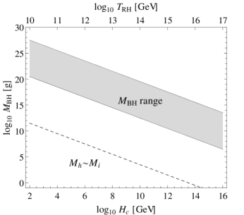
Figure 6: The range of characteristic masses of PBHs that can be produced by a hybrid inflation waterfall, as a function of inflation energy scale or reheating temperature.

5 Conclusions

We carried out numerical calculations of a contribution of the waterfall field to the primordial curvature perturbation (on uniform density hypersurfaces) $\zeta$, which is produced during waterfall transition in hybrid inflation scenario. The calculation is performed for a broad interval of values of the model parameters.

We did not consider the contribution to $\zeta$ from inflaton rolling, which is dominant at cosmological scales. One should note that the simple quadratic inflationary potential used in the present paper can be easily corrected (see, e.g., [50]) to give a red-tilted spectrum at cosmological scales (converting, e.g., the original hybrid inflation model to a hilltop model [51, 52]), without any modification of our predictions for small scales.

Main results of the paper are shown in figures 4, 5, 6. One can see from the figure 4 that peak amplitudes of ${\cal P}_{\zeta}$ strongly depend on the value of $\beta$ (curiously, ${\cal P}_{\zeta}\sim 1$ corresponds to $\beta\sim 1$ in a broad interval of $\gamma$ and $r$). The peak values, $k_{*}$, for small $\beta$ are far beyond horizon, so, the smoothing over the horizon size will not decrease the peak values of the smoothed spectrum. Furthermore, the spectrum near peak remains strongly non-Gaussian after the smoothing. Our calculations based on the quadratic inflaton potential show that for $\beta\lesssim 100$ and in the broad interval of $r$ the peak value $k_{*}$ can be estimated by the simple relation:

$$\frac{k_{*}}{aH}\sim e^{-N},$$ (5.1)

where $N$ is the number of e-folds during the waterfall transition. The similar estimate is contained in the recent work [8].

We conclude that the strong growth of amplitudes of the curvature perturbation spectrum at $\beta\to 1$, which had been anticipated in pioneering works [53, 54], really takes place. However, the condition which is very often used as a constraint, that the bare mass-squared of the $\chi$-field, $-m_{\chi}^{2}=2\sqrt{\lambda}M^{2}$, must be much larger than $H^{2}$ (the so-called “waterfall condition” [55]) seems to be too restrictive. Our results, presented in figures 4 and 5, show that only at $-m_{\chi}^{2}\approx H^{2}$ (when $\beta\sim 1$) the amplitude of the curvature spectrum ${\cal P}_{\zeta}$ becomes close to one, i.e., enters a region that can be constrained by PBH data. In figure 6 we show the region of PBH masses which can be produced due to the waterfall transition in hybrid inflation, in the case of large $\beta$ parameter. Abundances of these PBHs should be constrained by data of PBH searches. It would be very interesting to analyze the corresponding constraints following from data of relict GW searches (see, e.g., [26, 56, 57]).

References

- [1] D. H. Lyth, “Issues concerning the waterfall of hybrid inflation,” arXiv:1005.2461.
- [2] J. O. Gong and M. Sasaki, “Waterfall field in hybrid inflation and curvature perturbation,” JCAP 1103 (2011) 028 [arXiv:1010.3405].
- [3] J. Fonseca, M. Sasaki and D. Wands, “Large-scale Perturbations from the Waterfall Field in Hybrid Inflation,” JCAP 1009 (2010) 012 [arXiv:1005.4053].
- [4] A. A. Abolhasani and H. Firouzjahi, “No Large Scale Curvature Perturbations during Waterfall of Hybrid Inflation,” Phys. Rev. D 83 (2011) 063513 [arXiv:1005.2934].
- [5] A. A. Abolhasani, H. Firouzjahi and M. H. Namjoo, “Curvature Perturbations and non-Gaussianities from Waterfall Phase Transition during Inflation,” Class. Quant. Grav. 28 (2011) 075009 [arXiv:1010.6292].
- [6] D. H. Lyth, “Contribution of the hybrid inflation waterfall to the primordial curvature perturbation,” JCAP 1107 (2011) 035 [arXiv:1012.4617].
- [7] A. A. Abolhasani, H. Firouzjahi and M. Sasaki, “Curvature perturbation and waterfall dynamics in hybrid inflation,” arXiv:1106.6315.
- [8] D. H. Lyth, “Primordial black hole formation and hybrid inflation,” arXiv:1107.1681.
- [9] N. Barnaby and J. M. Cline, “Nongaussian and nonscale-invariant perturbations from tachyonic preheating in hybrid inflation,” Phys. Rev. D 73 (2006) 106012 [astro-ph/0601481].
- [10] N. Barnaby and J. M. Cline, “Nongaussianity from Tachyonic Preheating in Hybrid Inflation,” Phys. Rev. D 75 (2007) 086004 [astro-ph/0611750].
- [11] R. Kallosh, “On inflation in string theory,” Lect. Notes Phys. 738 (2008) 119-156 [hep-th/0702059].
- [12] R. Kallosh and A. D. Linde, “P term, D term and F term inflation,” JCAP 0310 (2003) 008 [hep-th/0306058].
- [13] J. H. Traschen and R. H. Brandenberger, “Particle Production During Out-of-equilibrium Phase Transitions,” Phys. Rev. D 42 (1990) 2491-2504.
- [14] A. D. Dolgov and D. P. Kirilova, “On Particle Creation By A Time Dependent Scalar Field,” Sov. J. Nucl. Phys. 51 (1990) 172-177 .
- [15] Y. Shtanov, J. H. Traschen and R. H. Brandenberger, “Universe reheating after inflation,” Phys. Rev. D 51 (1995) 5438-5455 [hep-ph/9407247].
- [16] L. Kofman, A. D. Linde and A. A. Starobinsky, “Reheating after inflation,” Phys. Rev. Lett. 73 (1994) 3195 [hep-th/9405187].
- [17] G. N. Felder, J. Garcia-Bellido, P. B. Greene, L. Kofman, A. D. Linde and I. Tkachev, “Dynamics of symmetry breaking and tachyonic preheating,” Phys. Rev. Lett. 87 (2001) 011601 [hep-ph/0012142].
- [18] B. A. Bassett, D. I. Kaiser, R. Maartens, “General relativistic preheating after inflation,” Phys. Lett. B 455 (1999) 84-89 [hep-ph/9808404].
- [19] A. R. Liddle, D. H. Lyth, K. A. Malik, D. Wands, “Superhorizon perturbations and preheating,” Phys. Rev. D 61 (2000) 103509 [hep-ph/9912473].
- [20] A. M. Green and K. A. Malik, “Primordial black hole production due to preheating,” Phys. Rev. D 64 (2001) 021301 [hep-ph/0008113].
- [21] L. Pilo, A. Riotto and A. Zaffaroni, “On the amount of gravitational waves from inflation,” Phys. Rev. Lett. 92 (2004) 201303 [astro-ph/0401302].
- [22] J. -O. Gong and M. Sasaki, “Curvature perturbation spectrum from false vacuum inflation,” JCAP 0901 (2009) 001 [arXiv:0804.4488].
- [23] T. Suyama, T. Tanaka, B. Bassett and H. Kudoh, “Are black holes over-produced during preheating?,” Phys. Rev. D 71 (2005) 063507 [hep-ph/0410247].
- [24] T. Suyama, T. Tanaka, B. Bassett and H. Kudoh, “Black hole production in tachyonic preheating,” JCAP 0604 (2006) 001 [hep-ph/0601108].
- [25] P. Brax, J. -F. Dufaux and S. Mariadassou, “Preheating after Small-Field Inflation,” Phys. Rev. D 83 (2011) 103510 [arXiv:1012.4656].
- [26] J. F. Dufaux, G. N. Felder, L. Kofman and O. Navros, “Gravity Waves from Tachyonic Preheating after Hybrid Inflation,” JCAP 0903 (2009) 001 [arXiv:0812.2917].
- [27] L. Kofman, A. D. Linde and A. A. Starobinsky, “Towards the theory of reheating after inflation,” Phys. Rev. D 56 (1997) 3258 [hep-ph/9704452].
- [28] T. Asaka, W. Buchmuller and L. Covi, “False vacuum decay after inflation,” Phys. Lett. B 510 (2001) 271-276 [hep-ph/0104037].
- [29] E. J. Copeland, S. Pascoli and A. Rajantie, “Dynamics of tachyonic preheating after hybrid inflation,” Phys. Rev. D 65 (2002) 103517 [hep-ph/0202031].
- [30] J. Garcia-Bellido, M. Garcia Perez and A. Gonzalez-Arroyo, “Symmetry breaking and false vacuum decay after hybrid inflation,” Phys. Rev. D 67 (2003) 103501 [hep-ph/0208228].
- [31] A. A. Starobinsky, “Dynamics of Phase Transition in the New Inflationary Universe Scenario and Generation of Perturbations,” Phys. Lett. B117 (1982) 175-178.
- [32] A. A. Starobinsky, “Multicomponent de Sitter (Inflationary) Stages and the Generation of Perturbations,” JETP Lett. 42 (1985) 152-155.
- [33] M. Sasaki and E. D. Stewart, “A General analytic formula for the spectral index of the density perturbations produced during inflation,” Prog. Theor. Phys. 95 (1996) 71 [astro-ph/9507001].
- [34] D. H. Lyth, K. A. Malik and M. Sasaki, “A General proof of the conservation of the curvature perturbation,” JCAP 0505 (2005) 004 [astro-ph/0411220].
- [35] A. D. Linde, “Axions in inflationary cosmology,” Phys. Lett. B 259 (1991) 38.
- [36] A. D. Linde, “Hybrid inflation,” Phys. Rev. D 49 (1994) 748-754 [astro-ph/9307002].
- [37] B. A. Bassett, S. Tsujikawa, D. Wands, “Inflation dynamics and reheating,” Rev. Mod. Phys. 78 (2006) 537-589 [astro-ph/0507632].
- [38] D. H. Lyth and A. R. Liddle, “The primordial density perturbation,” Cambridge University Press (2009).
- [39] D. H. Lyth, “Axions and inflation: Sitting in the vacuum,” Phys. Rev. D 45 (1992) 3394-3404.
- [40] D. Wands, K. A. Malik, D. H. Lyth and A. R. Liddle, “A New approach to the evolution of cosmological perturbations on large scales,” Phys. Rev. D 62 (2000) 043527 [astro-ph/0003278].
- [41] D. H. Lyth, A. Riotto, “Particle physics models of inflation and the cosmological density perturbation,” Phys. Rept. 314 (1999) 1-146 [hep-ph/9807278].
- [42] J. Garcia-Bellido, D. Wands, “Metric perturbations in two field inflation,” Phys. Rev. D 53 (1996) 5437-5445 [astro-ph/9511029].
- [43] M. Y. Khlopov, “Primordial Black Holes,” Res. Astron. Astrophys. 10 (2010) 495-528 [arXiv:0801.0116].
- [44] B. J. Carr, K. Kohri, Y. Sendouda and J. Yokoyama, “New cosmological constraints on primordial black holes,” Phys. Rev. D 81 (2010) 104019 [arXiv:0912.5297].
- [45] B. A. Bassett and S. Tsujikawa, “Inflationary preheating and primordial black holes,” Phys. Rev. D 63 (2001) 123503 [hep-ph/0008328].
- [46] F. Finelli and S. Khlebnikov, “Large metric perturbations from rescattering,” Phys. Lett. B 504 (2001) 309-313 [hep-ph/0009093].
- [47] B. J. Carr and S. W. Hawking, “Black holes in the early Universe,” Mon. Not. Roy. Astron. Soc. 168 (1974) 399-415.
- [48] J. C. Hidalgo, “The effect of non-Gaussian curvature perturbations on the formation of primordial black holes,” arXiv:0708.3875.
- [49] E. Bugaev and P. Klimai, “Constraints on amplitudes of curvature perturbations from primordial black holes,” Phys. Rev. D 79 (2009) 103511 [arXiv:0812.4247].
- [50] M. U. Rehman, Q. Shafi and J. R. Wickman, “Hybrid Inflation Revisited in Light of WMAP5,” Phys. Rev. D 79 (2009) 103503 [arXiv:0901.4345].
- [51] L. Boubekeur and D. H. Lyth, “Hilltop inflation,” JCAP 0507 (2005) 010 [hep-ph/0502047].
- [52] K. Kohri, C.-M. Lin and D. H. Lyth, “More hilltop inflation models,” JCAP 0712 (2007) 004 [arXiv:0707.3826].
- [53] L. Randall, M. Soljacic and A. H. Guth, “Supernatural inflation: Inflation from supersymmetry with no (very) small parameters,” Nucl. Phys. B 472 (1996) 377-408 [hep-ph/9512439].
- [54] J. Garcia-Bellido, A. D. Linde and D. Wands, “Density perturbations and black hole formation in hybrid inflation,” Phys. Rev. D 54 (1996) 6040-6058 [astro-ph/9605094].
- [55] E. J. Copeland, A. R. Liddle, D. H. Lyth, E. D. Stewart and D. Wands, “False vacuum inflation with Einstein gravity,” Phys. Rev. D 49 (1994) 6410-6433 [astro-ph/9401011].
- [56] E. Bugaev and P. Klimai, “Constraints on the induced gravitational wave background from primordial black holes,” Phys. Rev. D 83 (2011) 083521 [arXiv:1012.4697].
- [57] M. Giovannini, “Secondary graviton spectra and waterfall-like fields,” Phys. Rev. D 82 (2010) 083523 [arXiv:1008.1164].