Baryogenesis by $B-L$ generation due to superheavy particle decay

^aSeishi Enomoto , ^abNobuhiro Maekawa

^a Department of Physics, Nagoya University, Nagoya 464-8602, Japan

^b Kobayashi Maskawa Institute, Nagoya University, Nagoya 464-8602, Japan

We have shown that the $B-L$ generation due to the decay of the thermally produced superheavy fields can explain the Baryon assymmetry in the universe if the superheavy fields are heavier than $10^{13-14}$ GeV. Note that although the superheavy fields have non-vanishing charges under the standard model gauge interactions, the thermally prduced baryon asymmetry is sizable. The $B-L$ violating effective operators induced by integrating the superheavy fields have dimension 7, while the operator in the famous leptogenesis has dimension 5. Therefore, the constraints from the nucleon stability can be easily satisfied.

1 Introduction

To understand the origin of Baryon number $B$ in the universe is one of the most interesting subjects in the particle cosmology. The abundance of the Baryon in the universe is estimated by the nucleosynthesis analysis[1] and is observed by the WMAP[2], and it is quite impressive that they have given the consistent value for the Baryon density in the universe, which is roughly

$$\frac{n_{B}}{s}\sim 10^{-10},$$ (1.1)

where $n_{B}$ and $s$ are the Baryon number density and the entropy density, respectively. After Sakharov[3] pointed out the three conditions for the generation of the Baryon number $B$ in the universe, many mechanisms for baryogenesis have been studied in the literature[4, 5, 6, 7]. One of the most attractive scenario for the baryogenesis is the GUT baryogenesis[4] in which the decay of superheavy gauge bosons and Higgs appeared in the GUT produces the baryon number. Unfortunately, the produced baryon number is known to be washed out by the sphaleron process[8] in the standard model (SM). Since the sphaleron process conserves the $B-L$ number, it is important to produce non-vanishing $B-L$ number. The most famous scenario to produce $B-L$ number is the leptogenesis[5], in which the lepton number $L$ is produced by the decay of the right-handed neutrino. Especially, thermal leptogenesis, in which the lepton number is produced by the decay of the right-handed neutrino produced thermally, is one of the most interesting scenario because the observed baryon number can be related with the measurements on neutrino masses and mixings. However, since the scenarios in which the thermal leptogenesis can be applied are limited, other possibilities to produce the $B-L$ number are worth considering. In this paper, we study the $B-L$ production by the decay of certain superheavy fields with intermediate masses, which can be a remnant of some GUT models.

2 $B-L$ Violating Interactions

In the SM, the renormalizable operators cannot break the $B$ and $L$ numbers. Therefore, the non-conserving interactions appear in the higher dimensional operators whose mass dimensionis larger than four. For example, the dimension five operators $llh_{D}h_{D}$ between the doublet lepton $l$ and the doublet Higgs $h_{D}$ have non-vanishing $B-L$ charges and give neutrinos masses. The dimension 6 operators $qqu^{c\dagger}_{R}e^{c\dagger}_{R}$ break the $B$ and $L$ numbers, which can induce the proton decay. (For our notation of the particle contents, see Table 1.)

Names		$(SU(3)_{C},SU(2)_{L})_{U(1)_{Y}}$	$B$	$L$
doublet Quark	$q$	$(\mathbf{3},\mathbf{2})_{1/6}$	$+1/3$	$0$
right-handed Up	$u^{c}_{R}$	$(\bar{\mathbf{3}},\mathbf{1})_{-2/3}$	$-1/3$	$0$
right-handed Down	$d^{c}_{R}$	$(\bar{\mathbf{3}},\mathbf{1})_{1/3}$	$-1/3$	$0$
doublet Lepton	$l$	$(\mathbf{1},\mathbf{2})_{-1/2}$	$0$	$+1$
right-handed Electron	$e^{c}_{R}$	$(\mathbf{1},\mathbf{1})_{1}$	$0$	$-1$
doublet Higgs	$h_{D}$	$(\mathbf{1},\mathbf{2})_{1/2}$	$0$	$0$

Table 1: The particle contents and charges.

$llh_{D}h_{D}$ violates $L$ and $B-L$, while $qqu^{c\dagger}_{R}e^{c\dagger}_{R}$ violates $B$ and $L$ but not $B-L$. These higher dimensional operators, $llh_{D}h_{D}$ and $qqu^{c\dagger}_{R}e^{c\dagger}_{R}$, can be induced by integrating the superheavy right-handed neutrino $\nu_{R}^{c}$ and the GUT gauge boson $X$, respectively, as in Fig.1. The right-handed neutrino plays an important role in the leptogenesis scenario. And the $X$ gauge boson also plays a crucial role in the GUT baryogenesis.

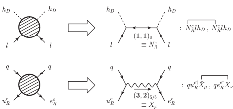
Figure 1: The decomposition of $llh_{D}h_{D}$ (upside) and $qqu_{R}^{c}e_{R}^{c}$ (downside). The fook over operators means the contraction.

Therefore, in order to produce $B-L$ number, it must be important to understand which superheavy particles can induce the $B-L$ violating higher dimensional operators.

Now, we discuss on other $B-L$ violating operators than $llh_{D}h_{D}$. In the literature, in the context of the nucleon decay, $B$ and/or $L$ violating operators have been classified in the SM[9] and in the minimal supersymmetric SM (MSSM)[10]. In the SM, there is no dimension six $B-L$ non-conserving operator. It is in dimension seven that we can find out $B-L$ non-conserving operators

$$qd_{R}^{c}llh_{D} \>,\>u_{R}^{c}d_{R}^{c}d_{R}^{c}lh_{D}\>,\>e_{R}^{c}lllh_{D}\>,\>qqd_{R}^{c\dagger}l^{\dagger}h_{D}^{\dagger}\>,\>qu_{R}^{c}l^{\dagger}l^{\dagger}h_{D}^{\dagger}\>,\>qe_{R}^{c}d_{R}^{c\dagger}d_{R}^{c\dagger}h_{D}^{\dagger}\>,$$

$$u_{R}^{c}e_{R}^{c}d_{R}^{c\dagger}l^{\dagger}h_{D}^{\dagger} \>,\>d_{R}^{c}d_{R}^{c}d_{R}^{c}lh_{D}^{\dagger}\>,\>qd_{R}^{c\dagger}d_{R}^{c\dagger}l^{\dagger}\>,\>u_{R}^{c}d_{R}^{c\dagger}l^{\dagger}l^{\dagger}\>,\>e_{R}^{c}d_{R}^{c\dagger}d_{R}^{c\dagger}d_{R}^{c\dagger}\>.$$

The last three operators include a differential operator or a gauge field. Since the differential operator can be replaced by the light fermion mass by using the equation of motion, the contribution of these operators become negligible and we do not consider the last three operators in the followings.

Which particles can induce these $B-L$ violating higher dimensional operators? To answer this question, let us decompose these operators into two parts. It is useful to write down these operators with the $SU(5)$ complete multiplets, ${\bf 10}\equiv(q,u_{R}^{c},e_{R}^{c})$, ${\bf\bar{5}}\equiv(d_{R}^{c},l)$, and ${\bf 5}_{s}\equiv(H_{T},h_{D})$, where $H_{T}$ is a colored Higgs, as ${\bf 10}\cdot{\bf\bar{5}}\cdot{\bf\bar{5}}\cdot{\bf\bar{5}}\cdot{\bf 5}_{s}$, ${\bf 10}\cdot{\bf 10}\cdot{\bf\bar{5}}^{\dagger}\cdot{\bf\bar{5}}^{\dagger}\cdot{\bf 5}^{\dagger}_{s}$, and ${\bf\bar{5}}\cdot{\bf\bar{5}}\cdot{\bf\bar{5}}\cdot{\bf\bar{5}}\cdot{\bf 5}_{s}^{\dagger}$. First of all, supposing that the superheavy fields are scalar. Then each part must includes two fermions. Therefore, the decomposition is limited. For example, the operator ${\bf 10}\cdot{\bf\bar{5}}\cdot{\bf\bar{5}}\cdot{\bf\bar{5}}\cdot{\bf 5}_{s}$ can be docomposed as $[{\bf 10}\cdot{\bf\bar{5}}\cdot{\bf 5}_{s}+{\bf\bar{5}}\cdot{\bf\bar{5}}]$ or $[{\bf 10}\cdot{\bf\bar{5}}+{\bf\bar{5}}\cdot{\bf\bar{5}}\cdot{\bf 5}_{s}]$. For simplicity, we assume that the superheavy fields are included in the $SU(5)$ multiplets, ${\bf 1}$, ${\bf 24}$, ${\bf 10}$, ${\bf 5}$. (Though it is straightforward to extend the superheavy fields with the general representations, we do not discuss the extension in detail in this paper.) For the former decomposition, the superheavy scalar belongs to ${\bf 10}$ representation of $SU(5)$, and for the latter, ${\bf 5}$. The concrete decompositions of the operators, $qd_{R}^{c}llh_{D}$ and $u_{R}^{c}d_{R}^{c}d_{R}^{c}lh_{D}$, can be seen in Fig.2 and 3, respectively.

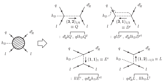
Figure 2: The decompositons of $qd_{R}^{c}llh_{D}$.

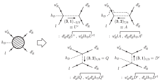
Figure 3: The decompositions of $u_{R}^{c}d_{R}^{c}d_{R}^{c}lh_{D}$.

We denote the superheavy fields as the large characters of the SM fields which have the same quantum numbers under the SM gauge interactions. (In Fig.3, the superheavy field $A$ has charges of $(\mathbf{3},\mathbf{2})_{7/6}$ under $SU(3)_{C}\times SU(2)_{L}\times U(1)_{Y}$, which belongs to $\mathbf{45}$ of $SU(5)$.) It is obvious that the superheavy scalars whose representations are ${\bf 10}$ or ${\bf 5}$ also induce the other $B-L$ violating operators. Therefore, we can consider the $B-L$ generation by the decay of the superheavy scalar fields which belong to ${\bf 10}$ and/or ${\bf 5}$ of $SU(5)$. We will return to this scenario in the next section.

If the superheavy fields are fermions, these operators must be decomposed as three fermions and one fermion. For example, the operator ${\bf 10}\cdot{\bf\bar{5}}\cdot{\bf\bar{5}}\cdot{\bf\bar{5}}\cdot{\bf 5}_{s}$ can be decomposed as $[{\bf 10}\cdot{\bf\bar{5}}\cdot{\bf\bar{5}}+{\bf\bar{5}}\cdot{\bf 5}_{s}]$ or $[{\bf\bar{5}}\cdot{\bf\bar{5}}\cdot{\bf\bar{5}}+{\bf 10}\cdot{\bf 5}_{s}]$. For the former decomposition, the superheavy fermions belong to ${\bf 1}$ or ${\bf 24}$, and for the latter, they belongs to ${\bf 10}$ and the complex conjugate. Actually the right-handed neutrinos which belongs to ${\bf 1}$ of $SU(5)$ can induce some of these operators. Though it must be possible to induce non-vanishing $B-L$ number by the decay of these superheavy fermions, we do not discuss this possibility in more detail. We may return to this subject in future.

In this section, we have decomposed the dimension seven $B-L$ violating operators into two parts. By this decomposition, we can address the generation of the $B-L$ number by the decay of the intermediate superheavy fields. Though some of the operators obtained by the decomposition have still higher dimension than four, we do not decompose them further because we do not need the origin of the operators to discuss $B-L$ generation.

3 $B-L$ Number Generation in the Early Universe

In this section, we study the $B-L$ generation by the decay of the superheavy scalar fields.

First, let us fix the particle contents. As discussed in the previous section, some additional fields are needed, and we introduce bosons denoted as $Q$, $U^{c}$, $D^{c}$, $E^{c}$, $L$ whose charges are the same as the Standard Model fermions, $q$, $u_{R}^{c}$, $d_{R}^{c}$, $e_{R}^{c}$, $l$, respectively.

Next, we write down all the dimension four and five interactions which include only one superheavy scalar as

• dim. 4 :
  $\quad d_{R}^{c}lQ\>,\>d_{R}^{c}d_{R}^{c}U^{c}\>,\>llE^{c}\>,\>qlD^{c}\>,\>u_{R}d_{R}D^{c}\>,\>q^{\dagger}q^{\dagger}D^{c}\>,\>u_{R}^{c\dagger}e_{R}^{c\dagger}D^{c}\>,$
  $\quad qd_{R}^{c}L\>,\>e_{R}^{c}lL\>,\>q^{\dagger}u_{R}^{c\dagger}L\>,\>(h.c.)$,

• dim. 5 :
  $\quad d_{R}^{c\dagger}d_{R}^{c\dagger}h_{D}Q\>,\>qqh_{D}^{\dagger}Q\>,\>u_{R}^{c}e_{R}^{c}h_{D}^{\dagger}Q\>,\>q^{\dagger}l^{\dagger}h_{D}^{\dagger}Q\>,\>u_{R}^{c\dagger}d_{R}^{c\dagger}h_{D}^{\dagger}Q\>,$
  $\quad d_{R}^{c\dagger}l^{\dagger}h_{D}U^{c}\>,\>qe_{R}^{c}h_{D}^{\dagger}U^{c}\>,\>u_{R}^{c\dagger}l^{\dagger}h_{D}^{\dagger}U^{c}\>,\>qu_{R}^{c}h_{D}^{\dagger}E^{c}\>,\>q^{\dagger}d_{R}^{c\dagger}h_{D}^{\dagger}E^{c}$
  $\quad e_{R}^{c\dagger}l^{\dagger}h_{D}^{\dagger}E^{c}\>,\>d_{R}^{c\dagger}l^{\dagger}h_{D}^{\dagger}D^{c}\>,\>l^{\dagger}l^{\dagger}h_{D}^{\dagger}L\>,\>(h.c.)$,

where we omited the indices of spinor, gauge of $SU(2)$ and $SU(3)$ for simplicity.

Interaction	$Q$	$U^{c}$	$E^{c}$	$D^{c}$	$L$
dim. 4	$+4/3$	$+2/3$	$\>\>+2\>\>$	$+2/3$	$0$
dim. 5	$-2/3$	$-4/3$	$0$	$-4/3$	$\>\>-2\>\>$

Table 2: The generated $B-L$ number by decay of additional particles.

It is interesting that the $B-L$ number of the final states by the decay of $Q$, $U^{c}$, $E^{c}$, $D^{c}$, $L$ is a fixed value for each superheavy fields and each dimension of the interactions as in Table 2. Since the $B-L$ number of the final states induced by the dimension four interactions is different from that by dimension five interactions, the decay can produce non-vanishing $B-L$ number.

For the estimation of the $B-L$ number, it is useful to calculate the mean net $B-L$ number $\epsilon$;

$$\epsilon_{i}=\sum_{f}x_{i\rightarrow f}\left[r(i\rightarrow f)-r(\bar{i}\rightarrow\bar{f})\right],$$ (3.1)

where $i$ is the initial decay particle with mass of $m_{i}$, which contains $Q$, $U^{c}$, $E^{c}$, $D^{c}$, $L$. $f$ means the decay modes from the decay of $i$. $x_{i\rightarrow f}$ is $B-L$ number within the decay modes $f$. $r$ is the branching ratio; $\bar{i}$ or $\bar{f}$ means $CP$ transformated state, i.e., anti-particles. $\epsilon_{i}$ means generated $B-L$ number for the decay of two particles $i$ and $\bar{i}$. Therefore, we can obtain the $B-L$ number density $n_{B-L}$ from the number density of the $i$ particle $n_{i}$ and the $\epsilon_{i}$ parameter as $n_{B-L}\sim\epsilon_{i}n_{i}$. After the sphaleron process, the $B$ number density $n_{B}$ is obtained as

$$n_{B}\sim 0.35n_{B-L}\sim 0.35\epsilon_{i}n_{i}.$$ (3.2)

Therefore, in order to obtain the $B$ number in a comoving frame $B\equiv\frac{n_{B}}{s}$, we have to know $\epsilon_{i}$ and $n_{i}$.

For the calculation of $\epsilon_{i}$, we denote couplings as follows;

where $y$ and $\lambda$ are dimensionless couplings, and $\Lambda$ is the scale of the higher dimensional interactions.

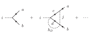
Figure 4: The Feynman diagrams for calculating $\epsilon_{i}$.

By calculating the Feynman diagrams in Fig. 4, we obtain $\epsilon_{i}$ as

$$\epsilon_{i}=\frac{2}{(8\pi)^{3}}\frac{m_{i}^{2}}{\Lambda^{2}}\frac{m_{i}}{16\pi\Gamma_{i}}\sum_{j,a,\dots,d}\textrm{Im}\left(\lambda_{jab}\lambda_{icb}^{\dagger}y_{jcd}^{\dagger}y_{ida}\right)\cdot f\left(m_{j}^{2}/m_{i}^{2}\right).$$ (3.3)

(See Appendix for the detail calculation. As an example if we take $i=Q$ and $j=U^{c}$, the summation becomes $\lambda_{Uld}\lambda_{Qdd}^{\dagger}y_{Udd}^{\dagger}y_{Qdl}+\lambda_{Ulu}\lambda_{Qdu}^{\dagger}y_{Udd}^{\dagger}y_{Qdl}$. We can also take $j=E^{c},D^{c},L$ for $i=Q$. Of course we can take $U^{c}$, $E^{c}$, $D^{c}$, $L$ as $i$. Once we fix the concrete fields as $i$ and $j$, the factor due to the number of freedom in the loop is appearing. We just ignore it in the following for simplicity.) $\Gamma_{i}$ is the total decay width;

$$\Gamma_{i}=\frac{m_{i}}{16\pi}\sum_{a,b}\left(y_{iab}^{\dagger}y_{iab}\right)+\frac{m_{i}}{3(8\pi)^{3}}\frac{m_{i}^{2}}{\Lambda^{2}}\sum_{a,b}\left(\lambda_{iab}^{\dagger}\lambda_{iab}\right),$$ (3.4)

where the first term is the contribution from the two body decay, and the second term is from the three body decay. Function $f$ in (3.3) is the loop function as follows;

$$f(\alpha) \equiv 1+2\alpha\left[1-(1+\alpha)\ln{\left(1+1/\alpha\right)}\right]$$ (3.5)

$$\sim \left\{\begin{array}[]{lr}1+\mathcal{O}(\alpha)&(\alpha\hskip 3.00003pt\raisebox{2.15277pt}{$<$}\raisebox{-3.22916pt}{{\footnotesize`}}\hskip 3.99994pt1)\\[2.84526pt] \frac{1}{3\alpha}+\mathcal{O}(1/\alpha^{2})&(\alpha\hskip 3.00003pt\raisebox{2.15277pt}{$>$}\raisebox{-3.22916pt}{{\footnotesize`}}\hskip 3.99994pt1)\end{array}\right..$$ (3.8)

If $m_{i}\sim m_{j}$ but $m_{i}<m_{j}$, then the function $f$ is rougly $\mathcal{O}(0.1)$.

Supposing that the only one coupling dominates the others for each $i$ particle and for each dimensional operator. Namely, there are four couplings, $y_{i}$, $y_{j}$, $\lambda_{i}$, and $\lambda_{j}$. Then, the eqs. (3.3) and (3.4) can be rewritten as

$$\epsilon_{i} = \frac{2}{(8\pi)^{3}}\frac{m_{i}^{2}}{\Lambda^{2}}\frac{m_{i}}{16\pi\Gamma_{i}}\textrm{Im}\left(\lambda_{j}\lambda_{i}^{\dagger}y_{j}^{\dagger}y_{i}\right)\cdot f\left(m_{j}^{2}/m_{i}^{2}\right),$$ (3.9)

$$\Gamma_{i} = \frac{m_{i}}{16\pi}|y_{i}|^{2}+\frac{m_{i}}{3(8\pi)^{3}}\frac{m_{i}^{2}}{\Lambda^{2}}|\lambda_{i}|^{2}.$$ (3.10)

Moreover, if we take $y\equiv|y_{i}|\sim|y_{j}|$ and $\lambda\equiv|\lambda_{i}|\sim|\lambda_{j}|$ and the branching ratio of two body decay is comparable to that of three body decay, i.e., $y\sim m_{i}\lambda/(4\sqrt{6}\pi\Lambda)$, then we can obtain simpler equations as

$$\Gamma_{i} \sim 2\frac{m_{i}}{16\pi}y^{2}.$$ (3.11)

$$\epsilon_{i} \sim \frac{3}{16\pi}y^{2}f\sin\delta,$$ (3.12)

where $\sin\delta\equiv\textrm{Im}\left(\lambda_{j}\lambda_{i}^{\dagger}y_{j}^{\dagger}y_{i}\right)/(y^{2}\lambda^{2})$.

Next, let us estimate the abundance of the $i$ particle, $n_{i}$, and the Baryon number in a comoving frame $B$ in the following two cases. In the first case, the particle $i$ is thermally produced, the freeze out occurs when the particle $i$ is still relativistic, and no entropy is produced by the decay (case A). (Therefore, we assume that the reheating temperature due to the inflation is larger than the mass of the superheavy particle $i$. We discuss whether the particle $i$ is still relativistic or not at the freeze out in section 4.) Then, $Y_{i}\equiv\frac{n_{i}}{s}$ is given by $Y_{i}\sim 0.278\frac{g_{eff}}{g_{*S}}$, where the entropy density $s$ is obtained as $s=\frac{2\pi^{2}}{45}g_{*S}T^{3}$ and $g_{eff}$ is the number of freedom of $i$. Therefore, we can obtain

$$B\sim 0.1\frac{g_{eff}\epsilon_{i}}{g_{*S}}\sim 3.5\times 10^{-5}y^{2},$$ (3.13)

where in the last similarity we use eq. (3.12), $f\sin\delta\sim 0.1$, $g_{*S}\sim 100$, and $g_{eff}\sim 6$ for $i=Q$. Therefore,

$$y\sim 2\times 10^{-3}$$ (3.14)

is required to obtain $B\sim 10^{-10}$. An additional condition $\Gamma_{i}>\langle\sigma v_{i}\rangle n_{i}$ is required so that the estimation $n_{B-L}\sim\epsilon_{i}n_{i}$ is valid, where $\sigma$ and $v_{i}$ are the cross section of the annihilation process and the velocity of the particle $i$, respectively. If $\langle\sigma v_{i}\rangle\sim 0.01T_{D}/m_{i}^{3}$, this condition is roughly rewritten as

$$\left(\frac{m_{i}}{M_{pl}}\right)^{2}>10^{-6}y^{2}.$$ (3.15)

Here, the decay temperature $T_{D}$ is defined by the temperature of the universe when the age of the universe is around the lifetime of the particle $i$, which is given by $T_{D}\sim\sqrt{\Gamma_{i}M_{pl}/1.66\sqrt{g_{*}}}$, where $M_{pl}$ is the Planck mass as $M_{pl}=1.22\times 10^{19}\>\rm{GeV}$. From the eq. (3.14), the inequality (3.15) is rewritten as

$$m_{i}>2\times 10^{-6}M_{pl}\sim 2\times 10^{13}\>\rm{GeV}.$$ (3.16)

When $m_{i}\sim 10^{14}(10^{16})$ GeV, $\Gamma_{i}\sim 10^{-7}m_{i}\sim 10^{7}(10^{9})$ GeV, and therefore, $T_{D}\sim 3\times 10^{12}(3\times 10^{13})$ GeV. The higher dimensional coupling is given as $\lambda/\Lambda\sim 4\sqrt{6}\pi y/m_{i}\sim 5\times 10^{-16}(5\times 10^{-18})({\rm GeV})^{-1}$.

As the second case (case B), we consider the situation in which the density of $i$ and $\bar{i}$ fields dominates the density of the universe. Generically, thermal abundance of the heavy particle with long lifetime becomes large and sometimes dominates the energy density of the universe. Then,

$$\rho=\rho_{i}+\rho_{\bar{i}}=2m_{i}n_{i}=\frac{\pi^{2}}{30}g_{*}T_{R}^{4},$$ (3.17)

where $\rho_{i}$, $\rho_{\bar{i}}$, $n_{i}$, $g_{*}$, and $T_{R}$ are the energy density of $i$ field, that of $\bar{i}$ field, the number density of $i$ field, the total number of effectively massless degrees of freedom, and the temperature after the $i$ and $\bar{i}$ field decay, respectively. The $B-L$ number in a comoving volume is given as

$$\frac{n_{B-L}}{s}=\frac{3}{8}\frac{g_{*}}{g_{*S}}\frac{T_{R}}{m_{i}}\epsilon_{i}.$$ (3.18)

After the sphaleron process, the $B$ number in a comoving volume is given as

$$B\equiv\frac{n_{B}}{s}\sim 0.35\frac{n_{B-L}}{s}\sim\frac{1}{8}\frac{T_{R}}{m_{i}}\epsilon_{i},$$ (3.19)

where we took $g_{*}\sim g_{*S}$. Therefore, the Baryon number is given by

$$B=\frac{3}{128\pi}\frac{y^{2}T_{R}}{m_{i}}f\sin\delta=\frac{3y^{3}}{256\sqrt{3.32}\pi^{1.5}g_{*}^{1/4}}\sqrt{\frac{M_{pl}}{m_{i}}}f\sin\delta\sim 4\times 10^{-5}\sqrt{\frac{M_{pl}}{m_{i}}}y^{3},$$ (3.20)

where the last similarity is given by taking $f\sin\delta\sim 0.1$ and $g_{*}=\mathcal{O}(100)$. Roughly, if we take

$$y^{3}\sqrt{M_{pl}/m_{i}}\sim 3\times 10^{-6},$$ (3.21)

then we can obtain $B\sim 10^{-10}$. The additional condition $\Gamma_{i}>\langle\sigma v_{i}\rangle n_{i}$ becomes

$$\left(\frac{m_{i}}{M_{pl}}\right)^{5}>10^{-12}y^{6}$$ (3.22)

by using eq. (3.17). From the eq. (3.21), the additional condition (3.22) is rewritten as

$$m_{i}>2\times 10^{-6}M_{pl}\sim 2\times 10^{13}\>\rm{GeV}.$$ (3.23)

When $m_{i}\sim 10^{14}(10^{16})$ GeV, the eq. (3.21) results in $y\sim 2(4)\times 10^{-3}$. Then $\Gamma_{i}\sim 2\times 10^{-7}(7\times 10^{-6})m_{i}\sim 2\times 10^{7}(7\times 10^{9})$ GeV, and therefore, $T_{R}\sim 3\times 10^{12}(7\times 10^{13})$ GeV. The higher dimensional coupling is given as $\lambda/\Lambda\sim 4\sqrt{6}\pi y/m_{i}\sim 6\times 10^{-16}(10^{-17})({\rm GeV})^{-1}$.

In this section, we have shown that the Baryon asymmetry in the universe can be explained by the $B-L$ production by the decay of some superheavy particle which can exist in some GUT models. .

4 Discussion and Summary

The initial density of the superheavy fields may be produced non-thermally like the preheating[11] and dominate the density of the universe. But here we consider the thermal abundance of the superheavy fields. If we take $\langle\sigma v_{i}\rangle\sim 0.01\frac{T}{(m_{i}^{2}+T^{2})^{\frac{3}{2}}}$, $g_{*}=g_{*S}=106.75$, and $g_{eff}=1$, then the numerical calculation shows that when the mass $m_{i}$ is larger than $10^{14}$ GeV the number density of the $i$ particle behaves like hot relics as $Y_{i}\sim 2\times 10^{-3}$ as in Table 3.

$m_{i}$(GeV)	$10^{11}$	$10^{12}$	$10^{13}$	$10^{14}$	$10^{15}$	$10^{16}$	Hot relics
$Y_{i}$($\times 10^{-3}$)	$0.019$	$0.10$	$0.46$	$1.4$	$2.0$	$2.1$	$2.2$

Table 3: Thermal abundance $Y_{i}$ with $y=0$.

In the numerical calculation, we used Boltzmann equations with Maxwell-Bolzmann approximation for the distribution function. Therefore, for this mass range, the calculation in case A is reasonable. But if $\frac{\rho_{i}+\rho_{\bar{i}}}{\rho_{R}}=\frac{8}{3}\frac{g_{eff}g_{*S}}{g_{*}}\frac{m_{i}}{T_{R}}Y_{i}>1$, then the calculation in case B is preferable because of the entropy production due to the decay of the particle $i$. Therefore, we conclude that thermal abundance of the superheavy fields is sufficient to explain the Baryon assymmetry in the universe. One of the point is that since the particles are superheavy, the Hubble expansion rate becomes so high that even gauge interactions can be out of equilibrium and not affect the generation of asymmetry. This is quite different from the usual leptogenesis.

If one of the right-handed neutrino masses is smaller than the decay temperature and $10^{12}$ GeV at which the sphaleron process becomes thermalized, then the produced $B-L$ number is washed out by the equilibrium of the $B-L$ violating neutrino process and the shaleron process[12]. Therefore, the mass of the right-handed neutrinos must be larger than the decay temperature in order to obtain the Baryon assymmetry by this mechanism if the right-handed neutrino is lighter than $10^{12}$ GeV.

The $B-L$ violating dimension 7 interactions via the superheavy fields, whose couplings are $y\lambda/(m_{i}^{2}\Lambda)$, can induce the instability of the nucleon. However, the contribution is negligible because the effective dimension 6 couplings become very small as $y\lambda\langle h_{D}\rangle/(m_{1}^{2}\Lambda)\ll 1/M_{pl}^{2}$.

In this paper, we do not introduce the supersymmetry(SUSY), but the extension to the SUSY models is straightforward. In some SUSY GUT models[13], there may be superheavy fields, $\bf 10+\bar{10}$, $\bf 24$, and $\bf 5+\bar{5}$ of $SU(5)$, some of which may produce the Baryon assymmetry in the universe, though the serious gravitino problem must be taken into account[14].

In this paper, we have studied the possibility that the decay of the superheavy particles, which may be induced in grand unified theories as extra fields, produces the non-vanishing $B-L$ number, which converts to the Baryon assymmetry by the shaleron process. We have shown that if the mass of the superheavy field is larger than $10^{13-14}$ GeV, the Baryon assymmetry in the universe can be explained by the decay of the superheavy field with appropriate couplings.

Appendix A The Calculation of the Mean Net $B-L$ Number

In this appendix, we will calculate the mean net $B-L$ number $\epsilon_{i}$ defined by

$$\epsilon_{i}=\sum_{f}x_{i\rightarrow f}(r_{i\rightarrow f}-r_{\bar{i}\rightarrow\bar{f}}).$$ (A.1)

Firstly let us simplify (A.1). The sum of the branching ratios of a group of decay modes $g$ which have the same $B-L$ charges $x_{i\rightarrow g}=const$ can be written

$$\sum_{g}r_{i\rightarrow g}=1-\sum_{f\neq g}r_{i\rightarrow f}.$$ (A.2)

Therefore, (A.1) is transformed to

$$\epsilon_{i} = x_{i\rightarrow g}\sum_{g}(r_{i\rightarrow g}-r_{\bar{i}\rightarrow\bar{g}})+\sum_{f\neq g}x_{i\rightarrow f}(r_{i\rightarrow f}-r_{\bar{i}\rightarrow\bar{f}})$$ (A.3)

$$= -x_{i\rightarrow g}\sum_{f\neq g}(r_{i\rightarrow f}-r_{\bar{i}\rightarrow\bar{f}})+\sum_{f\neq g}x_{i\rightarrow f}(r_{i\rightarrow f}-r_{\bar{i}\rightarrow\bar{f}})$$ (A.4)

$$= \sum_{f\neq g}(x_{i\rightarrow f}-x_{i\rightarrow g})(r_{i\rightarrow f}-r_{\bar{i}\rightarrow\bar{f}}).$$ (A.5)

Therefore, in calculating $\epsilon_{i}$, we do not have to calculate all the branching ratios.

In our case, modes $f$ run two and three body decays which are induced by dim.4 and 5 interactions respectively. Here, we choose the three body decays as modes $g$. Since $x_{i\rightarrow 2bd.}-x_{i\rightarrow 3bd.}=2$ for all species $i$ as is shown in Table 2, we obtain

$$\epsilon_{i} = 2\sum_{f=2bd.}(r_{i\rightarrow f}-r_{\bar{i}\rightarrow\bar{f}})$$ (A.6)

$$= 2\sum_{f=2bd.}(\Gamma_{i\rightarrow f}-\Gamma_{\bar{i}\rightarrow\bar{f}})/\Gamma_{i}$$ (A.7)

from (A.5), where $\Gamma_{i\rightarrow f}$ is the partial decay width and $\Gamma_{i}$ is the total decay width defined by

$$\Gamma_{i}\equiv\sum_{f}\Gamma_{i\rightarrow f}=\sum_{f}\Gamma_{\bar{i}\rightarrow\bar{f}}$$ (A.8)

Next, let us calculate difference of partial decay width $\Gamma_{i\rightarrow f}-\Gamma_{\bar{i}\rightarrow\bar{f}}$. In case of two body decays, the width is given by

$$\Gamma_{i\rightarrow f}=\frac{1}{16\pi m_{i}}\left|\mathcal{M}_{i\rightarrow f}\right|^{2},$$ (A.9)

where $\mathcal{M}$ is the amplitude. Here we assume that the decay products are massless. Using the following Feynman rules

the amplitude can be calculate as follows;

$$\left|\mathcal{M}_{i\rightarrow ab}\right|^{2} = \begin{array}[]{|c|}\includegraphics[scale={0.75}]{amplitude}\end{array}^{\>2}$$ (A.11)

$$= 2(p_{a}\cdot p_{b})\left|y_{iab}+\sum_{j,c,d}y_{jac}\frac{\lambda_{icd}}{\Lambda}\frac{\lambda_{jdb}^{\dagger}}{\Lambda}\mathcal{F}(m_{i},m_{j})+\cdots\right|^{2}$$ (A.12)

$$= m_{i}^{2}\left[\left|y_{iab}\right|^{2}+2\textrm{Re}\sum_{j,c,d}y_{iab}^{\dagger}y_{jac}\frac{\lambda_{icd}}{\Lambda}\frac{\lambda_{jdb}^{\dagger}}{\Lambda}\mathcal{F}(m_{i},m_{j})+\cdots\right],$$ (A.13)

where $\mathcal{F}$ is loop function. On the other hands, the amplitude for the anti-particle can be obtained by taking hermite conjugated couplings from the amplitude for the particle;

$$\left|\mathcal{M}_{\bar{i}\rightarrow\bar{a}\bar{b}}\right|^{2} = 2(p_{a}\cdot p_{b})\left|y_{iab}^{\dagger}+\sum_{j,c,d}y_{jac}^{\dagger}\frac{\lambda_{icd}^{\dagger}}{\Lambda}\frac{\lambda_{jdb}}{\Lambda}\mathcal{F}(m_{i},m_{j})+\cdots\right|^{2}$$ (A.14)

$$= m_{i}^{2}\left[\left|y_{iab}\right|^{2}+2\textrm{Re}\sum_{j,c,d}y_{iab}^{\dagger}y_{jac}\frac{\lambda_{icd}}{\Lambda}\frac{\lambda_{jdb}^{\dagger}}{\Lambda}\mathcal{F}^{\dagger}(m_{i},m_{j})+\cdots\right],$$ (A.15)

Using (A.9), (A.13) and (A.15), the difference of partial decay width can be written as

$$\Gamma_{i\rightarrow ab}-\Gamma_{\bar{i}\rightarrow\bar{a}\bar{b}} = \frac{1}{16\pi m_{i}}\left(\left|\mathcal{M}_{i\rightarrow ab}\right|^{2}-\left|\mathcal{M}_{\bar{i}\rightarrow\bar{a}\bar{b}}\right|^{2}\right)$$ (A.16)

$$= -\frac{m_{i}}{4\pi}\sum_{j,c,d}\textrm{Im}\left(y_{iab}^{\dagger}y_{jac}\frac{\lambda_{icd}}{\Lambda}\frac{\lambda_{jdb}^{\dagger}}{\Lambda}\right)\textrm{Im}\mathcal{F}(m_{i},m_{j})+\cdots$$ (A.17)

Here, $\textrm{Im}\mathcal{F}$ is given by

$$\textrm{Im}\mathcal{F}=-\frac{m_{i}^{2}}{2(8\pi)^{3}}f\left(m_{j}^{2}/m_{i}^{2}\right),$$ (A.18)

where $f$ is the function defined by (3.8). Note that the function $\mathcal{F}$ is diverging but $\textrm{Im}\mathcal{F}$ becomes finite. This is because the imaginary part can be estimated just by tree diagrams if Cutkosky rules are applied.

Finally, we can obtain the mean net $B-L$ number using (A.5), (A.17) and (A.18);

$$\epsilon_{i} = \frac{2}{(8\pi)^{3}}\frac{m_{i}^{2}}{\Lambda^{2}}\frac{m_{i}}{16\pi\Gamma_{i}}\sum_{j,a,\cdots,d}\textrm{Im}\left(y_{iab}^{\dagger}y_{jac}\lambda_{icd}\lambda_{jdb}^{\dagger}\right)f\left(m_{j}^{2}/m_{i}^{2}\right).$$ (A.19)

References

[1]
B. Fields and S. Sarkar,
J. Phys. G33, 1 (2006)
[arXiv:astro-ph/0601514].
[2]
D. N. Spergel et al. [WMAP Collaboration],
Astrophys. J. Suppl. 170, 377 (2007)
[arXiv:astro-ph/0603449].
[3]
A. D. Sakharov,
Pisma Zh. Eksp. Teor. Fiz. 5, 32 (1967)
[JETP Lett. 5, 24 (1967)]
[Sov. Phys. Usp. 34, 392 (1991)]
[Usp. Fiz. Nauk 161, 61 (1991)].
[4]
M. Yoshimura, Phys. Rev. Lett.41, 281(1978)
[Erratum-ibid. 42, 746 (1979)];
D. Toussaint, S. B. Treiman, F. Wilczek,
A. Zee, Phys. Rev. D19, 1036(1979); S. Weinberg,
Phys. Rev. Lett.42, 850(1979); S. Dimopoulos, L. Susskind,
Phys. Rev. D18, 4500(1978).
[5]
M. Fukugita, T. Yanagida,
Phys. Lett. B174, 45(1986).
[6]
V. A. Rubakov and M. E. Shaposhnikov,
Usp. Fiz. Nauk 166, 493 (1996)
[Phys. Usp. 39, 461 (1996)]
[arXiv:hep-ph/9603208].
[7]
I. Affleck, M. Dine, Nucl. Phys. B249, 361 (1985).
[8]
V.A. Kuzmin, V.A. Rubakov, M.A. Shaposhinikov,
Phys. Lett. B155, 36 (1985).
[9]
S. Weinberg, Phys. Rev. Lett.43, 1566 (1979);
Phys. Rev. D22, 1694 (1980);
F. Wilczek, A. Zee, Phys. Rev. Lett.43 1571 (1979).
[10]
N. Sakai, T. Yanagida, Nucl. Phys. B197, 533(1982);
S. Weinberg, Phys. Rev. D26, 287(1982).
[11]
L. Kofman, A. D. Linde and A. A. Starobinsky,
Phys. Rev. Lett. 73, 3195 (1994)
Phys. Rev. D56, 3258 (1997)
[12]
M. Fukugita, T. Yanagida, Phys. Rev. D42, 1285 (1990);
B.A. Campbell, S. Davidson, J. Ellis, K.A. Olive, Phys. Lett. B256,
457 (1991); Astroparticle Phys. 1, 77(1992).
[13]
N. Maekawa, Prog. Theor. Phys.106, 401-418 (2001); 107, 597-619 (2002);
N. Maekawa and T. Yamashita, Prog. Theor. Phys. 107, 1201-1233 (2002).
[14]
S. Weinberg,
Phys. Rev. Lett. 48, 1303 (1982);
I. V. Falomkin, G. B. Pontecorvo, M. G. Sapozhnikov, M. Y. Khlopov, F. Balestra and G. Piragino,
Nuovo Cim. A 79 (1984) 193
[Yad. Fiz. 39 (1984) 990];
M. Y. Khlopov and A. D. Linde,
Phys. Lett. B 138 (1984) 265;
J. R. Ellis, J. E. Kim and D. V. Nanopoulos,
Phys. Lett. B 145, 181 (1984).