Statistical Laws Governing Fluctuations in Word Use
from Word Birth to Word Death

Abstract

We analyze the dynamic properties of $10^{7}$ words recorded in English, Spanish and Hebrew over the period 1800–2008 in order to gain insight into the coevolution of language and culture. We report language independent patterns useful as benchmarks for theoretical models of language evolution. A significantly decreasing (increasing) trend in the birth (death) rate of words indicates a recent shift in the selection laws governing word use. For new words, we observe a peak in the growth-rate fluctuations around 40 years after introduction, consistent with the typical entry time into standard dictionaries and the human generational timescale. Pronounced changes in the dynamics of language during periods of war shows that word correlations, occurring across time and between words, are largely influenced by coevolutionary social, technological, and political factors. We quantify cultural memory by analyzing the long-term correlations in the use of individual words using detrended fluctuation analysis.

Statistical laws describing the properties of word use, such as Zipf’s law Zipf ; Zipfrecent ; PlosOneZipf ; 2regimeZipf ; variationZipf ; ScalingZipf and Heaps’ law HeapsOrig ; MetaHeaps , have been thoroughly tested and modeled. These statistical laws are based on static snapshots of written language using empirical data aggregated over relatively small time periods and comprised of relatively small corpora ranging in size from individual texts Zipf ; Zipfrecent to relatively small collections of topical texts PlosOneZipf ; 2regimeZipf . However, language is a fundamentally dynamic complex system, consisting of heterogenous entities at the level of the units (words) and the interacting users (us). Hence, we begin this paper with two questions: (i) Do languages exhibit dynamical patterns? (ii) Do individual words exhibit dynamical patterns?

The coevolutionary nature of language requires analysis both at the macro and micro scale. Here we apply interdisciplinary concepts to empirical language data collected in a massive book digitization effort by Google Inc., which recently unveiled a database of words in seven languages, after having scanned approximately 4% of the world’s books. The massive “n-gram” project googledata allows for a novel view into the growth dynamics of word use and the birth and death processes of words in accordance with evolutionary selection laws EvolLang .

A recent analysis of this database by Michel et al. googlepaper addresses numerous well-posed questions rooted in cultural anthropology using case studies of individual words. Here we take an alternative approach by analyzing the aggregate properties of the language dynamics recorded in the Google Inc. data in a systematic way, using the word counts of every word recorded over the 209-year time period 1800 – 2008 in the English, Spanish, and Hebrew text corpora. This period spans the incredibly rich cultural history that includes several international wars, revolutions, and numerous technological paradigm shifts. Together, the data comprise over $1\times 10^{7}$ distinct words. We use concepts from economics to gain quantitative insights into the role of exogenous factors on the evolution of language, combined with methods from statistical physics to quantify the competition arising from correlations between words WordnetlexiconHierarchy ; SemanticNetwork ; textHeirarchyCorr and the memory-driven autocorrelations in $u_{i}(t)$ across time FractalCorrCorpora ; ReturnIntervalsLanguage ; WordBursts .

For each corpora comprising millions of distinct words, we use a general word-count framework which accounts for the underlying growth of language over time. We first define the quantity $u_{i}(t)$ as the number of uses of word $i$ in year $t$. Since the number of books and the number of distinct words have grown dramatically over time, we define the relative word use, $f_{i}(t)$, as the fraction of uses of word $i$ out of all word uses in the same year,

$$f_{i}(t)\equiv u_{i}(t)/N_{u}(t)\ ,$$ (1)

where the quantity $N_{u}(t)\equiv\sum_{i=1}^{N_{w}(t)}u_{i}(t)$ is the total number of indistinct word uses digitized from books printed in year $t$ and $N_{w}(t)$ is the total number of distinct words digitized from books printed in year $t$. To quantify the dynamic properties of word prevalence at the micro scale and their relation to socio-political factors at the macro scale, we analyze the logarithmic growth rate commonly used in finance and economics,

$$r_{i}(t) \equiv \ln f_{i}(t+\Delta t)-\ln f_{i}(t)=\ln\Big{(}\frac{f_{i}(t+\Delta t)}{f_{i}(t)}\Big{)}\ .$$ (2)

The relative use $f_{i}(t)$ depends on the intrinsic grammatical utility of the word (related to the number of “proper” sentences that can be constructed using the word), the semantic utility of the word (related to the number of meanings a given word can convey), and other idiosyncratic details related to topical context. Neutral null models for the evolution of language define the relative use of a word as its “fitness” LanguageNeutralEvol . In such models, the word frequency is the only factor determining the survival capacity of a word. In reality, word competition depends on more subtle features of language, such as the cognitive aspects of efficient communication. For example, the emergence of robust categorical naming patterns observed across many cultures is regarded to be the result of complex discrimination tactics shared by intelligent communicators. This is evident in the finite set of words describing the continuous spectrum of color names, emotional states, and other categorical sets StatPhysLangDyn ; ColorNaming ; EmergenceTopicality .

In our analysis we treat words with equivalent meanings but with different spellings (e.g. color versus colour) as distinct words, since we view the competition among synonyms and alternative spellings in the linguistic arena as a key ingredient in complex evolutionary dynamics NowakLanguage ; EvolLang . For instance, with the advent of automatic spell-checkers in the digital era, words recognized by spell-checkers receive a significant boost in their “reproductive fitness” at the expense of their misspelled or unstandardized counterparts.

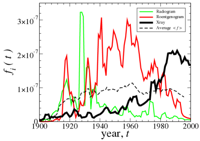
Figure 1: Word extinction. The English word “Roentgenogram” derives from the Nobel prize winning scientist and discoverer of the x-ray, Wilhelm Röntgen (1845–1923). The prevalence of this word was quickly challenged by two main competitors, “X-ray” (recorded as “Xray” in the database) and “Radiogram.” The arithmetic mean frequency of these three time series is relatively constant over the 80-year period 1920–2000, $\langle f\rangle\approx 10^{-7}$, illustrating the limited linguistic “market share” that can be achieved by any competitor. We conjecture that the main reason “Xray” has a higher frequency is due to the “fitness gain” from its efficient short word length and also due to the fact that English has become the base language for scientific publication.

In the linguistic arena, not just “defective” words die, even significantly used words can become extinct. Fig. 1 shows three once-significant words: “Radiogram,” “Roentgenogram,” and “Xray”. These words compete for the majority share of nouns referring to what is now commonly known as an “X-ray” (note that such dashes are discarded in Google’s digitization process). The word “Roentgenogram” has since become extinct, even though it was the most common term for several decades in the 20th century. It is likely that two main factors – (i) communication and information efficiency bias toward the use of shorter words efficientcommunication and (ii) the adoption of English as the leading global language for science – secured the eventual success of the word “Xray” by the year 1980. It goes without saying that there are many social and technological factors driving language change.

We begin this paper by analyzing the vocabulary growth of each language over time. We then analyze the lifetime growth trajectories of the set of words that are new to each language to gain quantitative insight into “infant” and “adult” stages of individual words. Using two sets of words, (i) the relatively new words, and (ii) the most common words, we analyze the statistical properties of word growth. Specifically, we calculate the probability density function $P(r)$ of growth rate $r$ and calculate the size-dependence of the standard deviation $\sigma(r)$ of growth rates. In order to gain insight into the long-term cultural memory, we conclude the analysis by measuring the autocorrelations in word use by applying detrended fluctuation analysis (DFA) to individual time series.

Results

Quantifying the birth rate and the death rate of words. Just as a new species can be born into an environment, a word can emerge in a language. Evolutionary selection laws can apply pressure on the sustainability of new words since there are limited resources (topics, books, etc.) for the use of words. Along the same lines, old words can be driven to extinction when cultural and technological factors limit the use of a word, in analogy to the environmental factors that can change the survival capacity of a living species by altering its ability to survive and reproduce.

Figure 2: Dramatic shift in the birth rate and death rate of words. The word birth rate $\gamma_{b}(t)$ and the word death rate $\gamma_{d}(t)$ show marked underlying changes in word use competition which affects the entry rate and the sustainability of existing words. The modern print era shows a marked increase in the death rate of words which likely correspond to low fitness, misspelled and (technologically) outdated words. A simultaneous decrease in the birth rate of new words is consistent with the decreasing marginal need for new words indicated by the sub-linear allometric scaling between vocabulary size and total corpus size (Heaps’ law) LanguageAll . Interestingly, we quantitatively observe the impact of the Balfour Declaration in 1917, the circumstances surrounding which effectively rejuvenated Hebrew as a national language, resulting in a 5-fold increase in the birth rate of words in the Hebrew corpus.

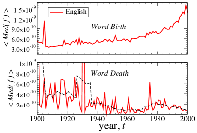
Figure 3: Survival of the fittest in the entry process of words. Trends in the relative uses of words that either were born or died in a given year show that the entry-exit forces largely depend on the relative use of the word. For the English corpus, we calculate the average of the median lifetime relative use, $\langle\text{Med}(f_{i})\rangle$, for all words born in year $t$ (top panel) and for all words that died in year $t$ (bottom panel), which shows a 5-year moving average (dashed black line). There is a dramatic increase in the relative use (“utility”) of newborn words over the last 20–30 years, likely corresponding to new technical terms, which are necessary for the communication of core modern technology and ideas. Conversely, with higher editorial standards and the recent use of word processors which include spelling standardization technology, the words that are dying are those words with low relative use. We confirm by visual inspection that the lists of dying words contain mostly misspelled and nonsensical words.

We define the birth year $y_{0,i}$ as the year $t$ corresponding to the first instance of $f_{i}(t)\geq 0.05f^{m}_{i}$, where $f^{m}_{i}$ is median word use $f^{m}_{i}=Median\{u_{i}(t)\}$ of a given word over its recorded lifetime in the Google database. Similarly, we define the death year $y_{f,i}$ as the last year $t$ during which the word use satisfies $f_{i}(t)\geq 0.05f^{m}_{i}$. We use the relative word use threshold $0.05f^{m}_{i}$ in order to avoid anomalies arising from extreme fluctuations in $f_{i}(t)$ over the lifetime of the word. The results obtained using threshold $0.10f^{m}_{i}$ did not show a significant qualitative difference.

The significance of word births $\Delta_{b}(t)$ and word deaths $\Delta_{d}(t)$ for each year $t$ is related to the vocabulary size $N_{w}(t)$ of a given language. We define the birth rate $\gamma_{b}$ and death rate $\gamma_{d}$ by normalizing the number of births and deaths in a given year $t$ to the total number of distinct words $N_{w}(t)$ recorded in the same year $t$, so that

$$\gamma_{b}(t)\equiv\Delta_{b}(t)/N_{w}(t)\ ,$$ (3)

$$\gamma_{d}(t)\equiv\Delta_{d}(t)/N_{w}(t)\ .$$

This definition yields a proxy for the rate of emergence and disappearance of words. We restrict our analysis to words with birth-death duration $y_{f,i}-y_{0,i}+1\geq 2$ years and to words with first recorded use $t_{0,i}\geq 1700$, which selects for relatively new words in the history of a language.

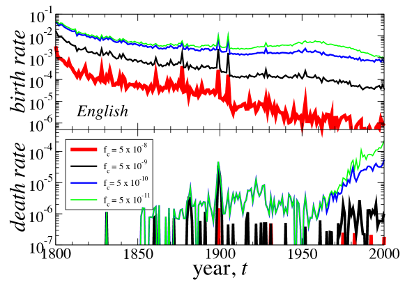
Figure S1: The birth and death rates of a word depends on the relative use of the word. For the English corpus, we calculate the birth and death rates for words with median lifetime relative use $\text{Med}(f_{i})$ satisfying $\text{Med}(f_{i})>f_{c}$. The difference in the birth rate curves corresponds to the contribution to the birth rate of words in between the two $f_{c}$ thresholds, and so the small difference in the curves for small $f_{c}$ indicates that the birth rate is largely comprised of words with relatively large $\text{Med}(f_{i})$. Consistent with this finding, the largest contribution to the death rate is from words with relatively low $\text{Med}(f_{i})$. By visually inspecting the lists of dying words, we confirm that words with large relative use rarely become completely extinct (see Fig. 1 for a counterexample word “Roentgenogram” which was once a frequently used word, but has since been eliminated due to competitive forces with other high-fitness competitors).

The $\gamma_{b}(t)$ and $\gamma_{d}(t)$ time series plotted in Fig. 2 for the 200-year period 1800–2000 show trends that intensifies after the 1950s. The modern era of publishing, which is characterized by more strict editing procedures at publishing houses, computerized word editing and automatic spell-checking technology, shows a drastic increase in the death rate of words. Using visual inspection we verify most changes to the vocabulary in the last 10–20 years are due to the extinction of misspelled words and nonsensical print errors, and to the decreased birth rate of new misspelled variations and genuinely new words. This phenomenon reflects the decreasing marginal need for new words, consistent with the sub-linear Heaps’ law observed for all Google 1-gram corpora in LanguageAll . Moreover, Fig. 3 shows that $\gamma_{b}(t)$ is largely comprised of words with relatively large median $f_{c}$ while $\gamma_{d}(t)$ is almost entirely comprised of words with relatively small median $f_{c}$ (see also Fig. S1 in the Supplementary Information (SI) text). Thus, the new words of tomorrow are likely be core words that are widely used.

We note that the main source of error in the calculation of birth and death rates are OCR (optical character recognition) errors in the digitization process, which could be responsible for a significant fraction of misspelled and nonsensical words existing in the data. An additional source of error is the variety of orthographic properties of language that can make very subtle variations of words, for example through the use of hyphens and capitalization, appear as distinct words when applying OCR. The digitization of many books in the computer era does not require OCR transfer, since the manuscripts are themselves digital, and so there may be a bias resulting from this recent paradigm shift. We confirm that the statistical patterns found using post 2000- data are consistent with the patterns that extend back several hundred years LanguageAll .

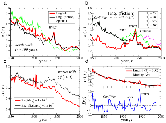
Figure 4: The significance of historical events on the evolution of language. The standard deviation $\sigma(t)$ of growth rates demonstrates the sensitivity of language to international events (e.g. World War II). For all languages there is an overall decreasing trend in $\sigma(t)$ over the period 1850–2000. However, the increase in $\sigma(t)$ during WWII represents a“globalization” effect, whereby societies are brought together by a common event and a unified media. Such contact between relatively isolated systems necessarily leads to information flow, much as in the case of thermodynamic heat flow between two systems, initially at different temperatures, which are then brought into contact. (a) $\sigma(t)$ calculated for the relatively new words with $T_{i}\geq 100$ years. The Spanish corpus does not show an increase in $\sigma(t)$ during World War II, indicative of the relative isolation of South America and Spain from the European conflict. (b) $\sigma(t)$ for 4 sets of relatively new words that meet the criteria $T_{i}\geq T_{c}$ and $t_{i,0}\geq 1800$. The oldest “new” words ($T_{c}=200$) demonstrate the most significant increase in $\sigma(t)$ during World War II, with a peak around 1945. (c) The standard deviation $\sigma(t)$ for the most common words is decreasing with time, suggesting that they have saturated and are being “crowding out” by new competitors. This set of words meets the criterion that the average relative use exceeds a threshold, $\langle f_{i}\rangle\geq f_{c}$, which we define for each corpus. (d) We compare the variation $\sigma(t)$ for relatively new English words, using $T_{i}\geq 100$, with the 20-year moving average over the time period 1820–1988. The deviations show that $\sigma(t)$ increases abruptly during times of conflict, such as the American Civil War (1861–1865), World War I (1914–1918) and World War II (1939–1945), and also during the 1980s and 1990s, possibly as a result of new digital media (e.g. the internet) which offer new environments for the evolutionary dynamics of word use. $D(t)$ is the difference between the moving average and $\sigma(t)$.

Complementary to the death of old words is the birth of new words, which are commonly associated with new social and technological trends. Topical words in media can display long-term persistence patterns analogous to earthquake shocks blogOmori ; BlogWordDynamics , and can result in a new word having larger fitness than related “out-of-date” words (e.g. blog vs. log, email vs. memo). Here we show that a comparison of the growth dynamics between different languages can also illustrate the local cultural factors that influence different regions of the world. Fig. 4 shows how international crisis can lead to globalization of language through common media attention and increased lexical diffusion. Notably, as illustrated in Fig. 4(a), we find that international conflict only perturbed the participating languages, while minimally affecting the languages of the nonparticipating regions, e.g. the Spanish speaking countries during WWII.

The lifetime trajectory of words. Between birth and death, one contends with the interesting question of how the use of words evolve when they are “alive.” We focus our efforts toward quantifying the relative change in word use over time, both over the word lifetime and throughout the course of history. In order to analyze separately these two time frames, we select two sets of words: (i) relatively new words with “birth year” $t_{0,i}$ later than 1800, so that the relative age $\tau\equiv t-t_{0,i}$ of word $i$ is the number of years after the word’s first occurrence in the database, and (ii) relatively common words, typically with $t_{0,i}<$ 1800.

We analyze dataset (i) words (summary statistics in Table S1) so that we can control for properties of the growth dynamics that are related to the various stages of a word’s life trajectory (e.g. an “infant” phase, an “adolescent” phase, and a “mature” phase). For comparison with the young words, we also analyze the growth rates of dataset (ii) words in the next section (summary statistics in Table S2). These words are presumably old enough that they are in a stable mature phase. We select dataset (ii) words using the criterion $\langle f_{i}\rangle\geq f_{c}$, where $\langle f_{i}\rangle=\sum_{\tau=1}^{T_{i}}f_{i}(\tau)/T_{i}$ is the average relative use of the word $i$ over the word’s lifetime $T_{i}=t_{0,f}-t_{0,i}+1$, and $f_{c}$ is a cutoff threshold derived form the Zipf rank-frequency distribution Zipf calculated for each corpus LanguageAll . In Table S3 we summarize the entire data for the 209-year period 1800–2008 for each of the four Google language sets analyzed.

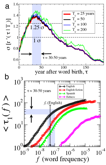
Figure 5: Quantifying the tipping point for word use. (a) The maximum in the standard deviation $\sigma$ of growth rates during the “adolescent” period $\tau\approx$ 30–50 indicates the characteristic time scale for words being incorporated into the standard lexicon, i.e. inclusion in popular dictionaries. In Fig. S4 we plot the average growth rate trajectory $\langle r^{\prime}(\tau|T_{c})\rangle$ which shows relatively large positive growth rates during approximately the same 20-year period. (b) The first passage time $\tau_{1}$ FirstPassage is defined as the number years for the relative use of a new word $i$ to exceed a given $f$-value for the first time, $f_{i}(\tau_{1})\geq f$. For relatively new words with $T_{i}\geq 100$ years we calculate the average first-passage time $\langle\tau_{1}(f)\rangle$ for a large range of $f$. We estimate for each language the $f_{c}$ representing the threshold for a word belonging to the standard “kernel” lexicon 2regimeZipf . This method demonstrates that the English corpus threshold $f_{c}\equiv 5\times 10^{-8}$ maps to the first passage time corresponding to the peak period $\tau\approx 30-50$ years in $\sigma(\tau)$ shown in panel (a).

Modern words typically are born in relation to technological or cultural events, e.g. “Antibiotics.” We ask if there exists a characteristic time for a word’s general acceptance. In order to search for patterns in the growth rates as a function of relative word age, for each new word $i$ at its age $\tau$, we analyze the “use trajectory” $f_{i}(\tau)$ and the “growth rate trajectory” $r_{i}(\tau)$. So that we may combine the individual trajectories of words of varying prevalence, we normalize each $f_{i}(\tau)$ by its average $\langle f_{i}\rangle$, obtaining a normalized use trajectory $f^{\prime}_{i}(\tau)\equiv f_{i}(\tau)/\langle f_{i}\rangle$. We perform an analogous normalization procedure for each $r_{i}(\tau)$, normalizing instead by the growth rate standard deviation $\sigma[r_{i}]$, so that $r^{\prime}_{i}(\tau)\equiv r_{i}(\tau)/\sigma[r_{i}]$ (see the Methods section for further detailed description).

Since some words will die and other words will increase in use as a result of the standardization of language, we hypothesize that the average growth rate trajectory will show large fluctuations around the time scale for the transition of a word into regular use. In order to quantify this transition time scale, we create a subset $\{i\ |T_{c}\}$ of word trajectories $i$ by combining words that meets an age criteria $T_{i}\geq T_{c}$. Thus, $T_{c}$ is a threshold to distinguish words that were born in different historical eras and which have varying longevity. For the values $T_{c}=25,50,100,$ and 200 years, we select all words that have a lifetime longer than $T_{c}$ and calculate the average and standard deviation for each set of growth rate trajectories as a function of word age $\tau$.

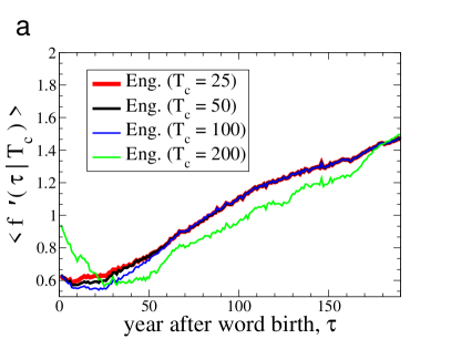
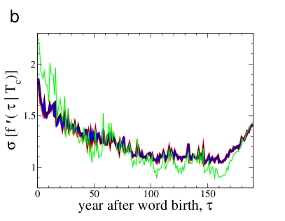
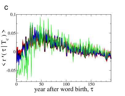
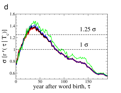
Figure S4: Statistical patterns in the growth trajectories of new words in the English corpus. Characteristics of the time-dependent word trajectory show the time scales over which a typical word becomes relevant or fades. For 4 values of $T_{c}$, we show the word trajectories for dataset (i) words in the English corpus, although the same qualitative results hold for the other languages analyzed. Recall that $T_{c}$ refers to the subset of timeseries with lifetime $T_{i}\geq T_{c}$, so that two trajectories calculated using different thresholds $T^{(1)}_{c}$ and $T^{(2)}_{c}$ only vary for $\tau<Max[T^{(1)}_{c},T^{(2)}_{c}]$. We show weighted average and standard deviations, using $\langle f_{i}\rangle$ as the weight for word $i$ contributing to the calculation of each time series in year $\tau$. (a) The relative use increases with time, consistent with the definition of the weighted average which biases towards words with large $\langle f_{i}\rangle$. For words with large $T_{i}$, the trajectory has a minimum which begins to reverse around $\tau\approx 40$ years, possibly reflecting the amount of time it takes to reach a critical utility threshold that corresponds to a relatively high fitness value for the word in relation to its competitors. (b) The variations in $\langle f(\tau|T_{c})\rangle$ decrease with time reflecting the transition from the insecure “infant” phase to the more secure “adult” phase in the lifetime trajectory. (c) The average growth trajectory is qualitatively related to the logarithmic derivative of the curve in panel (a), and confirms that the region of largest positive growth is $\tau\approx$ 30–50 years. (d) The variations in the average trajectory are larger than 1.25 $\sigma$ for $30\lesssim\tau\lesssim 50$ years and are larger than 1.0 $\sigma$ for $10\lesssim\tau\lesssim 80$ years. This regime of large fluctuations in the growth rates conceivably corresponds to the time period over which a successful word is accepted into the standard lexicon, e.g. a word included in an official dictionary or an idea/event recorded in an encyclopedia or review.

In Fig. 5 we plot $\sigma[r^{\prime}_{i}(\tau|T_{c})]$ for the English corpus, which shows a broad peak around $\tau_{c}\approx$ 30–50 years for each $T_{c}$ subset before the fluctuations saturate after the word enters a stable growth phase. A similar peak is observed for each corpus analyzed (Figs. S4–S7). This single-peak growth trajectory is consistent with theoretical models for logistic spreading and the fixation of words in a population of learners LangEcophysics . Also, since we weight the average according to $\langle f_{i}\rangle$, the time scale $\tau_{c}$ is likely associated with the characteristic time for a new word to reach sufficiently wide acceptance that the word is included in a typical dictionary. We note that this time scale is close to the generational time scale for humans, corroborating evidence that languages require only one generation to drastically evolve LangEcophysics .

Empirical laws quantifying the growth rate distribution. How much do the growth rates vary from word to word? The answer to this question can help distinguish between candidate models for the evolution of word utility. Hence, we calculate the probability density function (pdf) of $R\equiv r^{\prime}_{i}(\tau)/\sigma[r^{\prime}(\tau|T_{c})]$. Using this quantity accounts for the fact that we are aggregating growth rates of words of varying ages. The empirical pdf $P(R)$ shown in Fig. 6 is leptokurtic and remarkably symmetric around $R\approx 0$. These empirical facts are also observed in studies of the growth rates of economic institutions Growth1b ; Growth6 ; Growth1 ; GrowthEcon . Since the $R$ values are normalized and detrended according to the age-dependent standard deviation $\sigma[r^{\prime}(\tau|T_{c})]$, the standard deviation is $\sigma(R)=1$ by construction.

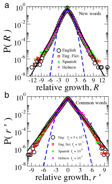
Figure 6: Common leptokurtic growth distribution for new words and common words. (a) Independent of language, the growth rates of relatively new words are distributed according to the Laplace distribution centered around $R\approx 0$ defined in Eq. (4). The the growth rate $R$ defined in Eq. (11) is measured in units of standard deviation, and accounts for age-dependent and word-dependent factors. Yet, even with these normalizations, we still observe an excess number of $|R|\geq 3\sigma$ events. This fact is demonstrated by the leptokurtic form of each $P(R)$, which exhibit the excess tail frequencies when compared with a unit-variance Gaussian distribution (dashed blue curve). The Gaussian distribution is the predicted distribution for the Gibrat proportional growth model, which is a candidate neutral null-model for the growth dynamics of word use Growth6 . The prevalence of large growth rates illustrate the possibility that words can have large variations in use even over the course of a year. The growth variations are intrinsically related to the dynamics of everyday life and reflect the cultural and technological shocks in society. We analyze word use data over the time period 1800-2008 for new words $i$ with lifetimes $T_{i}\geq T_{c}$, where we show data calculated for $T_{c}=100$ years. (b) PDF $P(r^{\prime})$ of the annual relative growth rate $r^{\prime}$ for all words which satisfy $\langle f_{i}\rangle\geq f_{c}$ (dataset #ii words which are relatively common words). In order to select relatively frequently used words, we use the following criteria: $T_{i}\geq 10$ years, $1800\leq t\leq 2008$, and $\langle f_{i}\rangle\geq f_{c}$. The growth rate $r^{\prime}$ does not account for age-dependent factors since the common words are likely in the mature phase of their lifetime trajectory. In each panel, we plot a Laplace distribution with unit variance (solid black lines) and the Gaussian distribution with unit variance (dashed blue curve) for reference.

A candidate model for the growth rates of word use is the Gibrat proportional growth process Growth1 ; Growth6 , which predicts a Gaussian distribution for $P(R)$. However, we observe the “tent-shaped” pdf $P(R)$ which is well-approximated by a Laplace (double-exponential) distribution, defined as

$$P(R)\equiv\frac{1}{\sqrt{2}\sigma(R)}\exp[-\sqrt{2}|R-\langle R\rangle|/\sigma(R)]\ .$$ (4)

Here the average growth rate $\langle R\rangle$ has two properties: (a) $\langle R\rangle\approx 0$ and (b) $\langle R\rangle\ll\sigma(R)$. Property (a) arises from the fact that the growth rate of distinct words is quite small on the annual basis (the growth rate of books in the Google English database is $\gamma_{w}\approx 0.011$ LanguageAll ) and property (b) arises from the fact that $R$ is defined in units of standard deviation. Being leptokurtic, the Laplace distribution predicts an excess number of events $>3\sigma$ as compared to the Gaussian distribution. For example, comparing the likelihood of events above the $3\sigma$ event threshold, the Laplace distribution displays a five-fold excess in the probability $P(|R-\langle R\rangle|>3\sigma)$, where $P(|R-\langle R\rangle|>3\sigma)=\exp[-3\sqrt{2}]\approx 0.014$ for the Laplace distribution, whereas $P(|R-\langle R\rangle|>3\sigma)=\text{Erfc}[3/\sqrt{2}]\approx 0.0027$ for the Gaussian distribution. The large $R$ values correspond to periods of rapid growth and decline in the use of words during the crucial “infant” and “adolescent” lifetime phases. In Fig. 6(b) we also show that the growth rate distribution $P(r^{\prime})$ for the relatively common words comprising dataset (ii) is also well-described by the Laplace distribution.

For hierarchical systems consisting of units each with complex internal structure Growth2 (e.g. a given country consists of industries, each of which consists of companies, each of which consists of internal subunits), a non-trivial scaling relation between the standard deviation of growth rates $\sigma(r|S)$ and the system size $S$ has the form

$$\sigma(r|S_{i})\sim S_{i}^{-\beta}\ .$$ (5)

The theoretical prediction in Growth2 ; Growth11 that $\beta\in[0,1/2]$ has been verified for several economic systems, with empirical $\beta$ values typically in the range $0.1<\beta<0.3$ Growth11 .

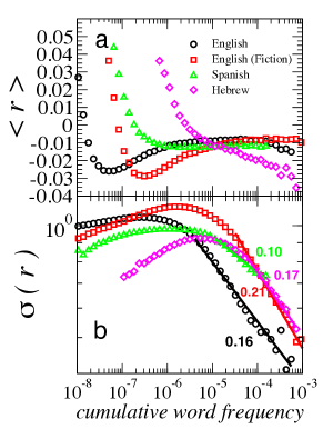
Figure 7: Scaling in the growth rate fluctuations of words. We show the dependence of growth rates on the cumulative word frequency $S_{i}\equiv\sum_{t^{\prime}=0}^{t}f_{i}(t)$ using words satisfy the criteria $T_{i}\geq 10$ years. We verify similar results for threshold values $T_{c}=50,100$, and $200$ years. (a) Average growth rate $\langle r\rangle$ saturates at relatively constant values for large $S$. (b) Scaling in the standard deviation of growth rates $\sigma(r|S)\sim S^{-\beta}$ for words with large $S$. This scaling relation is also observed for the growth rates of large economic institutions, ranging in size from companies to entire countries GrowthEcon ; Growth11 . Here this size-variance relation corresponds to scaling exponent values $0.10<\beta<0.21$, which are related to the non-trivial bursting patterns and non-trivial correlation patterns in literature topicality as indicated by the quantitative relation to the Hurst exponent, $H=1-\beta$ shown in scalinghumaninteraction . We calculate $\beta_{Eng.}\approx 0.16\pm 0.01$, $\beta_{Eng.fict}\approx 0.21\pm 0.01$, $\beta_{Spa.}\approx 0.10\pm 0.01$ and $\beta_{Heb.}\approx 0.17\pm 0.01$.

Since different words have varying lifetime trajectories as well as varying relative utilities, we now quantify how the standard deviation $\sigma(r|S_{i})$ of growth rates $r$ depends on the cumulative word frequency

$$S_{i}\equiv\sum_{\tau=1}^{T_{i}}f_{i}(\tau)\ ,$$ (6)

of each word. We choose this definition for proxy of “word size” since a writer can learn and recall a given word through any of its historical uses. Hence, $S_{i}$ is also proportional to the number of books in which word $i$ appears. This is significantly different than the assumptions of replication null models (e.g. the Moran process) which use the concurrent frequency $f_{i}(t)$ as the sole factor determining the likelihood of future replication EvolLang ; LanguageNeutralEvol .

We estimate Eq. (5) by grouping words according to $S_{i}$ and then calculating the growth rate standard deviation $\sigma(r|S_{i})$ for each group. Fig. 7(b) shows scaling behavior consistent with Eq. 5 for large $S_{i}$, with $\beta\approx$ 0.10 – 0.21 depending on the corpus. A positive $\beta$ value means that words with larger cumulative word frequency have smaller annual growth rate fluctuations. We conjecture that this statistical pattern emerges from the hierarchical organization of written language WordnetlexiconHierarchy ; SemanticNetwork ; textHeirarchyCorr ; FractalCorrCorpora ; ReturnIntervalsLanguage and the social properties of the speakers who use the words MetaHeaps ; WordNiche ; WordBursts . As such, we calculate $\beta$ values that are consistent with nontrivial correlations in word use, likely related to the basic fact that books are topical PlosOneZipf and that book topics are correlated with cultural trends.

Quantifying the long-term cultural memory. Recent theoretical work scalinghumaninteraction shows that there is a fundamental relation between the size-variance exponent $\beta$ and the Hurst exponent $H$ quantifying the auto-correlations in a stochastic time series. The novel relation $H=1-\beta$ indicates that the temporal long-term persistence is intrinsically related to the capability of the underlying mechanism to absorb stochastic shocks. Hence, positive correlations ($H>1/2$) are predicted for non-trivial $\beta$ values (i.e. $0\leq\beta\leq 0.5$). Note that the Gibrat proportional growth model predicts $\beta=0$ and that a Yule-Simon urn model predicts $\beta=0.5$ Growth11 . Thus, $f_{i}(\tau)$ belonging to words with large $S_{i}$ are predicted to show significant positive correlations, $H_{i}>1/2$.

To test this connection between memory correlations and the size-variance scaling, we calculate the Hurst exponent $H_{i}$ for each time series belonging to the more relatively common words analyzed in dataset (ii) using detrended fluctuation analysis (DFA) DFA1 ; DFA2 ; scalinghumaninteraction . We plot in Fig. S2 the relative use time series $f_{i}(t)$ for the words “polyphony,” “Americanism,” “Repatriation,” and “Antibiotics” along with DFA curves from which we calculate each $H_{i}$. Fig. S2(b) shows that the $H_{i}$ values for these four words are all significantly greater than $H_{r}=0.5$, which is the expected Hurst exponent for a stochastic time series with no temporal correlations. In Fig. S3 we plot the distribution of $H_{i}$ values for the English fiction corpus and the Spanish corpus. Our results are consistent with the theoretical prediction $\langle H\rangle=1-\beta$ established in scalinghumaninteraction relating the variance of growth rates to the underlying temporal correlations in each $f_{i}(t)$. Hence, we show that the language evolution is fundamentally related to the complex features of cultural memory, i.e. the dynamics of cultural topic formation WordNiche ; WordBursts ; blogOmori ; BlogWordDynamics and bursting Barabasibursts ; SornettePNAS .

Discussion

With the digitization of written language, cultural trend analysis based around methods to extract quantitative patterns from word counts is an emerging interdisciplinary field that has the potential to provide novel insights into human sociology PlosOneZipf ; WordBursts ; WordNiche ; blogOmori ; BlogWordDynamics ; TwitterWords . Nevertheless, the amount of metadata extractable from daily internet feeds is dizzying. This is highlighted by the practical issue of defining objective significance levels to filter out the noise in the data deluge. For example, online blogs can be vaguely categorized according to the coarse hierarchical schema: “obscure blogs”, “more popular blogs”, “tech columns”, and “mainstream news coverage.” In contrast, there are well-defined entry requirements for published books and magazines, which must meet editorial standards and conform to the principles of market supply and demand. However, until recently, the vast information captured in the annals of written language was largely inaccessible.

Despite the careful guard of libraries around the world, which house the written corpora for almost every written language, little is known about the aggregate dynamics of word evolution in written history. Inspired by research on the growth patterns displayed by a wide range of competition driven systems - from countries and business firms GrowthEcon ; Growth3 ; Growth1b ; Growth6 ; Growth1 ; Growth2 ; Growth11 ; GrowthBuldPamm ; Growth13b ; lgcmps99 to religious activities Growth10 , universities Growth12 , scientific journals Growth7 , careers careerscaling and bird populations BirdGrowth - here we extend the concepts and methods to word use dynamics.

This study provides empirical evidence that words are competing actors in a system of finite resources. Just as business firms compete for market share, words demonstrate the same growth statistics because they are competing for the use of the writer/speaker and for the attention of the corresponding reader/listener StatPhysLangDyn ; ColorNaming ; EmergenceTopicality ; LanguageNeutralEvol ; LangEcophysics . A prime example of fitness-mediated evolutionary competition is the case of irregular and regular verb use in English. By analyzing the regularization rate of irregular verbs through the history of the English language, Lieberman et al. Evodynamicslanguage show that the irregular verbs that are used more frequently are less likely to be overcome by their regular verb counterparts. Specifically, they find that the irregular verb death rate scales as the inverse square root of the word’s relative use. A study of word diffusion across Indo-European languages shows similar frequency-dependence of word replacement rates lexdiffusion .

We document the case example of X-ray, which shows how categorically related words can compete in a zero-sum game. Moreover, this competition does not occur in a vacuum. Instead, the dynamics are significantly related to diffusion and technology. Lexical diffusion occurs at many scales, both within relatively small groups and across nations lexdiffusion ; WordNiche ; LangEcophysics . The technological forces underlying word selection have changed significantly over the last 20 years. With the advent of automatic spell-checkers in the digital era, words recognized by spell-checkers receive a significant boost in their “reproductive fitness” at the expense of their “misspelled” or unstandardized counterparts.

We find that the dynamics are influenced by historical context, trends in global communication, and the means for standardizing that communication. Analogous to recessions and booms in a global economy, the marketplace for words waxes and wanes with a global pulse as historical events unfold. And in analogy to financial regulations meant to limit risk and market domination, standardization technologies such as the dictionary and spell checkers serve as powerful arbiters in determining the characteristic properties of word evolution. Context matters, and so we anticipate that niches WordNiche in various language ecosystems (ranging from spoken word to professionally published documents to various online forms such as chats, tweets and blogs) have heterogenous selection laws that may favor a given word in one arena but not another. Moreover, the birth and death rate of words and their close associates (misspellings, synonyms, abbreviations) depend on factors endogenous to the language domain such as correlations in word use to other partner words and polysemous contexts WordnetlexiconHierarchy ; SemanticNetwork as well as exogenous socio-technological factors and demographic aspects of the writers, such as age SemanticNetwork and social niche WordNiche .

We find a pronounced peak in the fluctuations of word growth rates when a word has reached approximately 30-50 years of age (see Fig. 5). We posit that this corresponds to the timescale for a word to be accepted into a standardized dictionary which inducts words that are used above a threshold frequency, consistent with the first-passage times to $f_{c}$ in Fig. 5(b). This is further corroborated by the characteristic baseline frequencies associated with standardized dictionaries googlepaper . Another important timescale in evolutionary systems is the reproduction age of the interacting gene or meme host. Interestingly, a 30-50 year timescale is roughly equal to the characteristic human generational time scale. The prominent role of new generation of speakers in language evolution has precedent in linguistics. For example, it has been shown that primitive pidgin languages, which are little more than crude mixes of parent languages, spontaneously acquire the full range of complex syntax and grammar once they are learned by the children of a community as a native language. It is at this point a pidgin becomes a creole, in a process referred to as nativization NowakLanguage .

Nativization also had a prominent effect in the revival of the Hebrew language, a significant historical event which also manifests prominently in our statistical analysis. The birth rate of new words in the Hebrew language jumped by a factor of 5 in just a few short years around 1920 following the Balfour Declaration of 1917 and the Second Aliyah immigration to Israel. The combination of new Hebrew-speaking communities and political endorsement of a national homeland for the Jewish people in the Palestine Mandate had two resounding affects: (i) the Hebrew language, hitherto used largely only for (religious) writing, gained official status as a modern spoken language, and (ii) a centralized culture emerged from this national community. The unique history of the Hebrew language in concert with the Google Inc. books data thus provide an unprecedented opportunity to quantitatively study the emerging dynamics of what is, in some regards, a new language.

The impact of historical context on language dynamics is not limited to emerging languages, but extends to languages that have been active and evolving continuously for a thousand years. We find that historical episodes can drastically perturb the properties of existing languages over large time scales. Moreover, recent studies show evidence for short-timescale cascading behavior in blog trends blogOmori ; BlogWordDynamics , analogous to the aftershocks following earthquakes and the cascades of market volatility following financial news announcements OmoriFOMC . The nontrivial autocorrelations and the leptokurtic growth distributions demonstrate the significance of exogenous shocks which can result in growth rates that significantly exceeding the frequencies that one would expect from non-interacting proportional growth models Growth1 ; Growth6 .

A large number of the world’s ethnic groups are separated along linguistic lines. A language barrier can isolate its speakers by serving as a screen to external events, which may further slow the rate of language evolution by stalling endogenous change. Nevertheless, we find that the distribution of word growth rates significantly broadens during times of large scale conflict, revealed through the sudden increases in $\sigma(t)$ for the English, French, German and Russian corpora during World War II LanguageAll . This can be understood as manifesting from the unification of public consciousness that creates fertile breeding ground for new topics and ideas. During war, people may be more likely to have their attention drawn to global issues. Remarkably, the pronounced change during WWII was not observed for the Spanish corpus, documenting the relatively small roles that Spain and Latin American countries played in the war.

Methods

Quantifying the word use trajectory. Once a word is introduced into a language, what are the characteristic growth patterns? To address this question, we first account for important variations in words, as the growth dynamics may depend on the frequency of the word as well as social and technological aspects of the time-period during which the word was born.

Here we define the age or trajectory year $\tau=t-t_{0,i}$ as the number of years after the word’s first appearance in the database. In order to compare trajectories across time and across varying word frequency, we normalize the trajectories for each word $i$ by the average use

$$\langle f_{i}\rangle\equiv\frac{1}{T_{i}}\sum_{t=t_{0,i}}^{t_{f,i}}f_{i}(t)$$ (7)

over the lifetime $T_{i}\equiv t_{f,i}-t_{0,i}+1$ of the word, leading to the normalized trajectory,

$$f^{\prime}_{i}(\tau)=f^{\prime}_{i}(t-t_{i,0}|t_{i,0},T_{i})\equiv f_{i}(t-t_{i,0})/\langle f_{i}\rangle\ .$$ (8)

By analogy, in order to compare various growth trajectories, we normalize the relative growth rate trajectory $r^{\prime}_{i}(t)$ by the standard deviation over the entire lifetime,

$$\sigma[r_{i}]\equiv\sqrt{\frac{1}{T_{i}}\sum_{t=t_{0,i}}^{t_{f,i}}[r_{i}(t)-\langle r_{i}\rangle]^{2}}\ .$$ (9)

Hence, the normalized relative growth trajectory is

$$r^{\prime}_{i}(\tau)=r^{\prime}_{i}(t-t_{i,0}|t_{i,0},T_{i})\equiv r_{i}(t-t_{i,0})/\sigma[r_{i}]\ .$$ (10)

Figs. S4-S7 show the weighted averages $\langle f^{\prime}(\tau|T_{c})\rangle$ and $\langle r^{\prime}(\tau|T_{c})\rangle$ and the weighted standard deviations $\sigma[f^{\prime}(\tau|T_{c})]$ and $\sigma[r^{\prime}(\tau|T_{c})]$ calculated using normalized trajectories for new words in each corpus. We compute $\langle\dotsb\rangle$ and $\sigma[\dotsb]$ for each trajectory year $\tau$ using all $N_{t}$ trajectories (Table S1) that satisfy the criteria $T_{i}\geq T_{c}$ and $t_{i,0}\geq 1800$. We compute the weighted average and the weighted standard deviation using $\langle f_{i}\rangle$ as the weight value for word $i$, so that $\langle\dotsb\rangle$ and $\sigma[\dotsb]$ reflect the lifetime trajectories of the more common words that are “new” to each corpus.

Since there is an intrinsic word maturity $\sigma[r^{\prime}(\tau|T_{c})]$ that is not accounted for in the quantity $r^{\prime}_{i}(\tau)$, we further define the detrended relative growth

$$R\equiv r^{\prime}_{i}(\tau)/\sigma[r^{\prime}(\tau|T_{c})]$$ (11)

which allows us to compare the growth factors for new words at various life stages. The result of this normalization is to rescale the standard deviations for a given trajectory year $\tau$ to unity for all values of $r^{\prime}_{i}(\tau)$.

Detrended fluctuation analysis of individual $f_{i}(t)$. Here we outline the DFA method for quantifying temporal autocorrelations in a general time series $f_{i}(t)$ that may have underlying trends, and compare the output with the results expected from a time series corresponding to a 1-dimensional random walk.

In a time interval $\delta t$, a time series $Y(t)$ deviates from the previous value $Y(t-\delta t)$ by an amount $\delta Y(t)\equiv Y(t)-Y(t-\delta t)$. A powerful result of the central limit theorem, equivalent to Fick’s law of diffusion in 1 dimension, is that if the displacements are independent (uncorrelated corresponding to a simple Markov process), then the total displacement $\Delta Y(t)=Y(t)-Y(0)$ from the initial location $Y(0)\equiv 0$ scales according to the total time $t$ as

$$\Delta Y(t)\equiv Y(t)\sim t^{1/2}\ .$$ (12)

However, if there are long-term correlations in the time series $Y(t)$, then the relation is generalized to

$$\Delta Y(t)\sim t^{H}\ ,$$ (13)

where $H$ is the Hurst exponent which corresponds to positive correlations for $H>1/2$ and negative correlations for $H<1/2$.

Since there may be underlying social, political, and technological trends that influence each time series $f_{i}(t)$, we use the detrended fluctuation analysis (DFA) method DFA1 ; DFA2 ; scalinghumaninteraction to analyze the residual fluctuations $\Delta f_{i}(t)$ after we remove the local trends. The method detrends the time series using time windows of varying length $\Delta t$. The time series $\tilde{f}_{i}(t|\Delta t)$ corresponds to the locally detrended time series using window size $\Delta t$. We calculate the Hurst exponent $H$ using the relation between the root-mean-square displacement $F(\Delta t)$ and the window size $\Delta t$ DFA1 ; DFA2 ; scalinghumaninteraction ,

$$F(\Delta t)=\sqrt{\langle\Delta\tilde{f}_{i}(t|\Delta t)^{2}\rangle}=\Delta t^{H}\ .$$ (14)

Here $\Delta\tilde{f}_{i}(t|\Delta t)$ is the local deviation from the average trend, analogous to $\Delta Y(t)$ defined above.

Fig. S2 shows 4 different $f_{i}(t)$ in panel (a), and plots the corresponding $F_{i}(\Delta t)$ in panel (b). The calculated $H_{i}$ values for these 4 words are all significantly greater than the uncorrelated $H=0.5$ value, indicating strong positive long-term correlations in the use of these words, even after we have removed the local trends using DFA. In these example cases, the trends are related to political events such as war in the cases of “Americanism” and “Repatriation”, or the bursting associated with new technology in the case of “Antibiotics,” or new musical trends illustrated in the case of “polyphony.”

In Fig. S3 we plot the pdf of $H_{i}$ values calculated for the relatively common words analyzed in Fig. 6(b). We also plot the pdf of $H_{i}$ values calculated from shuffled time series, and these values are centered around $\langle H\rangle\approx 0.5$ as expected from the removal of the intrinsic temporal ordering. Thus, using this method, we are able to quantify the social memory characterized by the Hurst exponent which is related to the bursting properties of linguistic trends, and in general, to bursting phenomena in human dynamics blogOmori ; BlogWordDynamics ; Barabasibursts ; SornettePNAS .

Acknowledgments
We thank Will Brockman, Fabio Pammolli, Massimo Riccaboni, and Paolo Sgrignoli for critical comments and insightful discussions. We gratefully acknowledge financial support from the U.S. DTRA and the IMT Foundation.

Author Contributions
A. M. P., J. T., S. H. & H. E. S., designed research, performed research, wrote, reviewed and approved the manuscript. A. M. P. and J. T. performed the numerical and statistical analysis of the data.

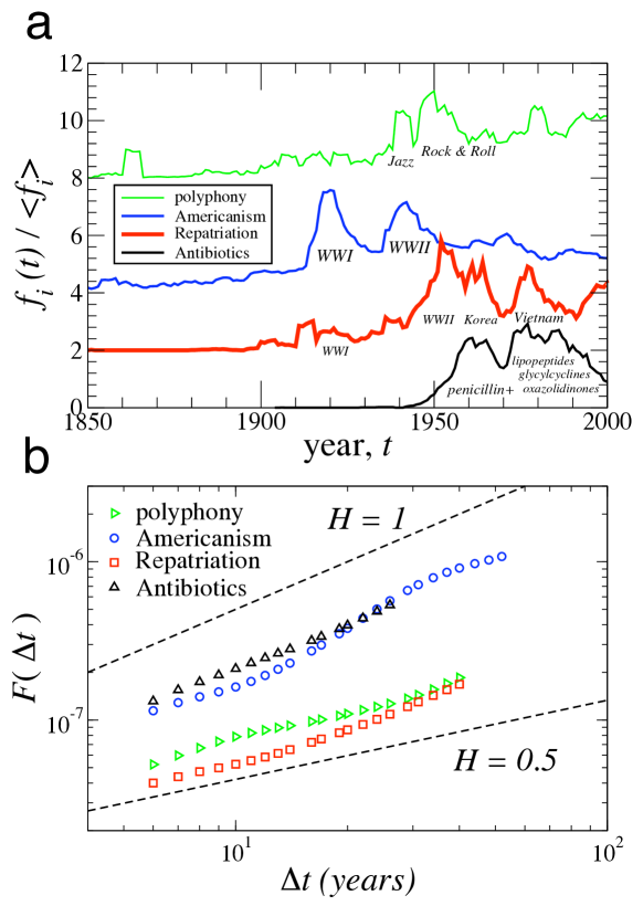
Figure S2: Measuring the social memory effect using the trajectories of single words. We measure the Hurst exponent for individual $f_{i}(t)$ using the detrended fluctuation analysis method DFA1 ; DFA2 ; scalinghumaninteraction . (a) Four example $f_{i}(t)$, given in units of the average use $\langle f_{i}\rangle$, show bursting of use as a result of social and political “shock” events. We choose these four examples based on their relatively large $H_{i}>0.5$ values. The use of “polyphony” in the English corpus shows peaks during the eras of jazz and rock and roll. The use of “Americanism” shows bursting during times of war, and the use of “Repatriation” shows an approximate 10-year lag in the bursting after WWII and the Vietnam War. The use of the word “Antibiotics” is related to technological advancement. The top 3 curves are vertically displaced by a constant from the value $f_{i}(1800)\approx 0$ so that the curves can be distinguished. (b) We use detrended fluctuation analysis (DFA) to calculate the Hurst exponent $H_{i}$ for each word in order to quantify the long-term correlations (“memory”) in each $f_{i}(t)$ time series. Fig. S3 shows the probability density function $P(H)$ of $H_{i}$ values calculated for the relatively common words found in English fiction and Spanish, summarized in Table S2.

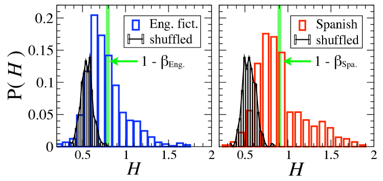
Figure S3: Individual Hurst exponents $H_{i}$ indicate a strong positively correlated memory underlying word use dynamics. Results of detrended fluctuation analysis (DFA) DFA1 ; DFA2 ; scalinghumaninteraction on the common [dataset (ii)] words analyzed in Fig. 6(b) show strong long-term memory with positive correlations, since $H>1/2$, indicating strong correlated bursting in the dynamics of word use, likely compounded by historical, social, or technological events. We calculate $\langle H_{i}\rangle\pm\sigma=0.77\pm 0.23$ (Eng. fiction) and $\langle H_{i}\rangle=0.90\pm 0.29$ (Spanish). The size-variance $\beta$ values calculated from the data in Fig. 7 confirm the theoretical prediction $\langle H\rangle=1-\beta$ in scalinghumaninteraction . Fig. 7 shows that $\beta_{Eng.fict}\approx 0.21\pm 0.01$ and $\beta_{Spa.}\approx 0.10\pm 0.01$. For the shuffled time series, we calculate $\langle H_{i}\rangle\pm\sigma=0.55\pm 0.07$ (Eng. fiction) and $\langle H_{i}\rangle\pm\sigma=0.55\pm 0.08$ (Spanish), which are consistent with time series that lack temporal ordering (memory).

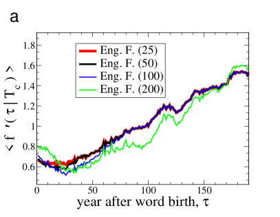
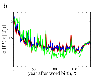
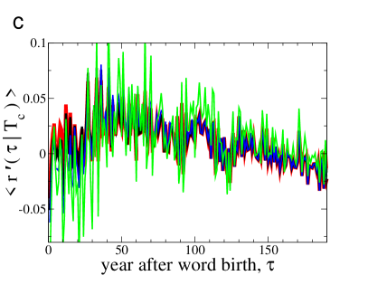
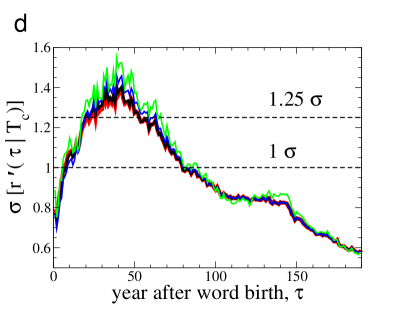
Figure S5: Statistical patterns in the growth trajectories of new words in the English Fiction corpus.

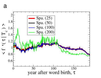
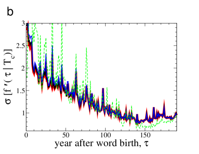
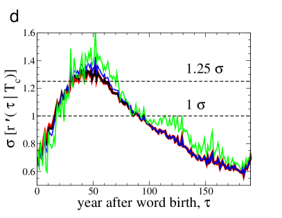
Figure S6: Statistical patterns in the growth trajectories of new words in the Spanish corpus.

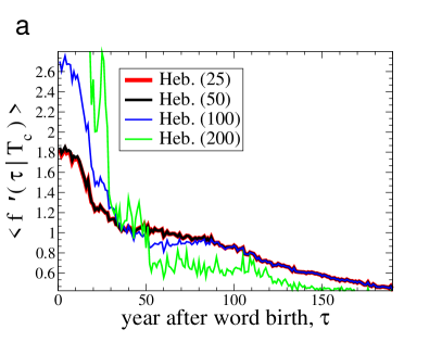
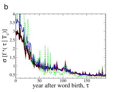
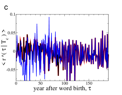
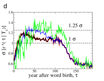
Figure S7: Statistical patterns in the growth trajectories of new words in the Hebrew corpus.

Table S1: Summary of annual growth trajectory data for varying threshold $T_{c}$, and $s_{c}=0.2$, $Y_{0}\equiv 1800$ and $Y_{f}\equiv 2008$.

Annual growth $R(t)$ data
Corpus,
(1-grams)	$T_{c}(years)$	$N_{t}(words)$	% (of all words)	$N_{R}(values)$	$\langle R\rangle$	$\sigma[R]$
English	25	302,957	4.1	31,544,800	$2.4\times 10^{-3}$	1.00
English fiction	25	99,547	3.8	11,725,984	$-3.0\times 10^{-3}$	1.00
Spanish	25	48,473	2.2	4,442,073	$1.8\times 10^{-3}$	1.00
Hebrew	25	29,825	4.6	2,424,912	$-3.6\times 10^{-3}$	1.00
English	50	204,969	2.8	28,071,528	$-1.7\times 10^{-3}$	1.00
English fiction	50	72,888	2.8	10,802,289	$-1.7\times 10^{-3}$	1.00
Spanish	50	33,236	1.5	3,892,745	$-9.3\times 10^{-4}$	1.00
Hebrew	50	27,918	4.3	2,347,839	$-5.2\times 10^{-3}$	1.00
English	100	141,073	1.9	23,928,600	$1.0\times 10^{-4}$	1.00
English fiction	100	53,847	2.1	9,535,037	$-8.5\times 10^{-4}$	1.00
Spanish	100	18,665	0.84	2,888,763	$-2.2\times 10^{-3}$	1.00
Hebrew	100	4,333	0.67	657,345	$-9.7\times 10^{-3}$	1.00
English	200	46,562	0.63	9,536,204	$-3.8\times 10^{-3}$	1.00
English fiction	200	21,322	0.82	4,365,194	$-3.5\times 10^{-3}$	1.00
Spanish	200	2,131	0.10	435,325	$-3.1\times 10^{-3}$	1.00
Hebrew	200	364	0.06	74,493	$-1.4\times 10^{-2}$	1.00

Table S2: Summary of data for the relatively common words that meet the criterion that their average word use $\langle f_{i}\rangle$ over the entire word history is larger than a threshold $f_{c}$, defined for each corpus. In order to select relatively frequently used words, we use the following three criteria: the word lifetime $T_{i}\geq 10$ years, $1800\leq t\leq 2008$, and $\langle f_{i}\rangle\geq f_{c}$.

Data summary for relatively common words
Corpus,
(1-grams)	$f_{c}$	$N_{t}(words)$	% (of all words)	$N_{r^{\prime}}(values)$	$\langle r^{\prime}\rangle$	$\sigma[r^{\prime}]$
English	$5\times 10^{-8}$	106,732	1.45	16,568,726	1.19 $\times 10^{-2}$	0.98
English fiction	$1\times 10^{-7}$	98,601	3.77	15,085,368	5.64 $\times 10^{-3}$	0.97
Spanish	$1\times 10^{-6}$	2,763	0.124	473,302	9.00 $\times 10^{-3}$	0.96
Hebrew	$1\times 10^{-5}$	70	0.011	6,395	3.49 $\times 10^{-2}$	1.00

Table S3: Summary of Google corpus data. Annual growth rates correspond to data in the 209-year period 1800–2008.

	Annual use $u_{i}(t)$ 1-gram data					Annual growth $r(t)$ data
Corpus,
(1-grams)	$N_{u}(uses)$	$Y_{i}$	$Y_{f}$	$N_{w}(words)$	$Max[u_{i}(t)]$	$N_{r}(values)$	$\langle r\rangle$	$\sigma[r]$
English	$3.60\times 10^{11}$	1520	2008	7,380,256	824,591,289	310,987,181	$2.21\times 10^{-2}$	$0.98$
English fiction	$8.91\times 10^{10}$	1592	2009	2,612,490	271,039,542	122,304,632	$2.32\times 10^{-2}$	$1.03$
Spanish	$4.51\times 10^{10}$	1532	2008	2,233,564	74,053,477	111,333,992	$7.51\times 10^{-3}$	$0.91$
Hebrew	$2.85\times 10^{9}$	1539	2008	645,262	5,587,042	32,387,825	$9.11\times 10^{-3}$	$0.90$

References

- (1) G. K. Zipf, Human Behaviour and the Principle of Least Effort: An Introduction to Human Ecology (Addison-Wesley, Cambridge, MA 1949).
- (2) Tsonis, A. A., Schultz, C., Tsonis, P. A. Zipf’s law and the structure and evolution of languages. Complexity 3, 12–13 (1997).
- (3) Serrano, M.Á., Flammini, A., Menczer, F. Modeling Statistical Properties of Written Text. PLoS ONE 4(4), e5372 (2009).
- (4) Ferrer i Cancho, R., Solé, R. V. Two regimes in the frequency of words and the origin of complex lexicons: Zipf’s law revisited. Journal of Quantitative Linguistics 8, 165–173 (2001).
- (5) Ferrer i Cancho, R. The variation of Zipf’s law in human language. Eur. Phys. J. B 44, 249–257 (2005).
- (6) Ferrer i Cancho, R., Solé, R. V. Least effort and the origins of scaling in human language. Proc. Natl. Acad. Sci. USA 100, 788–791(2003).
- (7) Heaps, H. S. Information Retrieval: Computational and Theoretical Aspects. (Academic Press, New York NY, 1978).
- (8) Bernhardsson, S., Correa da Rocha, L. E., Minnhagen, P. The meta book and size-dependent properties of written language. New J. of Physics 11, 123015 (2009).
- (9) Google n-gram project. http://ngrams.googlelabs.com
- (10) Nowak, M. A. Evolutionary Dynamics: exploring the equations of life (BelknapHarvard, Cambridge MA, 2006).
- (11) Michel, J.-B., et al. Quantitative Analysis of Culture Using Millions of Digitized Books. Science 331, 176–182 (2011).
- (12) Sigman, M., Cecchi, G. A. Global organization of the Wordnet lexicon. Proc. Natl. Acad. Sci. 99, 1742–1747 (2002).
- (13) Steyvers, M., Tenenbaum, J. B. The large-scale structure of semantic networks: statistical analyses and a model of semantic growth. Cogn. Sci. 29 41–78 (2005).
- (14) Alvarez-Lacalle, E., Dorow, B., Eckmann, J.-P., Moses, E. Hierarchical structures induce long-range dynamical correlations in written texts. Proc. Natl. Acad. Sci. 103, 7956–7961 (2006).
- (15) Montemurro, M. A., Pury, P. A. Long-range fractal correlations in literary corpora. Fractals 10, 451–461 (2002).
- (16) Corral, A., Ferrer i Cancho, R., Diaz-Guilera, A. Universal complex structures in written language. e-print, arXiv:0901.2924v1 (2009).
- (17) Altmann, E. G., Pierrehumbert, J. B., Motter, A. E. Beyond word frequency: bursts, lulls, and scaling in the temporal distributions of words. PLoS ONE 4, e7678 (2009).
- (18) Blythe, R. A. Neutral evolution: a null model for language dynamics. To appear in ACS Advances in Complex Systems.
- (19) Loreto, V., Baronchelli, A., Mukherjee, A., Puglisi, A., Tria, F. Statistical physics of language dynamics. J. Stat. Mech. 2011, P04006 (2011).
- (20) Baronchelli, A., Loreto, V., Steels, L. In-depth analysis of the Naming Game dynamics: the homogenous mixing case. Int. J. of Mod. Phys. C 19, 785–812 (2008).
- (21) Puglisi, A., Baronchelli, A., Loreto, V. Cultural route to the emergence of linguistic categories. Proc. Natl. Acad. Sci. 105, 7936–7940 (2008).
- (22) Nowak, M. A., Komarova, N. L., Niyogi, P. Computational and evolutionary aspects of language. Nature 417, 611–617 (2002).
- (23) Piantadosi, S. T., Tily, H., Gibson, E. Word lengths are optimized for efficient communication Proc. Natl. Acad. Sci. USA 108, 3526–3529 (2011).
- (24) Petersen, A. M., Tenenbaum, J., Havlin, S., Stanley, H. E. In preparation, see the SI materials for the e-print: arXiv:1107.3707 Version 1
- (25) Klimek, P., Bayer, W., Thurner, S. The blogosphere as an excitable social medium: Richter’s and Omori’s Law in media coverage. Physica A 390, 3870–3875 (2011).
- (26) Sano, Y., Yamada, K., Watanabe, H., Takayasu, H., Takayasu, M. Empirical analysis of collective human behavior for extraordinary events in blogosphere. (preprint) arXiv:1107.4730 [physics.soc-ph].
- (27) Solé, R. V., Corominas-Murtra, B., Fortuny, J. Diversity, competition, extinction: the ecophysics of language change. J. R. Soc. Interface 7, 1647–1664 (2010).
- (28) Amaral, L. A. N., et al. Scaling Behavior in Economics: I. Empirical Results for Company Growth. J. Phys. I France 7, 621–633 (1997).
- (29) Fu, D., et al., The growth of business firms: Theoretical framework and empirical evidence. Proc. Natl. Acad. Sci. 102, 18801–18806 (2005).
- (30) Stanley, M. H. R., et al. Scaling behaviour in the growth of companies. Nature 379, 804–806 (1996).
- (31) Canning, D., et al. Scaling the volatility of gdp growth rates. Economic Letters 60, 335–341 (1998).
- (32) Amaral, L. A. N., et al. Power Law Scaling for a System of Interacting Units with Complex Internal Structure. Phys. Rev. Lett. 80, 1385–1388 (1998).
- (33) Riccaboni, M., et al. The size variance relationship of business firm growth rates. Proc. Natl. Acad. Sci. 105, 19595–19600 (2008).
- (34) Altmann, E. G., Pierrehumbert, J. B., Motter, A. E. Niche as a determinant of word fate in online groups. PLoS ONE 6, e19009 (2011).
- (35) Rybski, D., et al. Scaling laws of human interaction activity. Proc. Natl. Acad. Sci. USA 106, 12640–12645 (2009).
- (36) Peng, C. K., et al. Mosaic organization of DNA nucleotides. Phys. Rev. E 49, 1685 – 1689 (1994).
- (37) Hu, K., et al. Effect of Trends on Detrended Fluctuation Analysis. Phys. Rev. E 64, 011114 (2001).
- (38) Barabási, A. L. The origin of bursts and heavy tails in human dynamics. Nature 435, 207–211 (2005).
- (39) Crane, R., Sornette, D. Robust dynamic classes revealed by measuring the response function of a social system. Proc. Natl. Acad. Sci. 105, 15649–15653 (2008) .
- (40) Golder, S. A., Macy, M. W. Diurnal and Seasonal Mood Vary with Work, Sleep, and Daylength Across Diverse Cultures. Science 333, 1878–1881 (2011).
- (41) Buldyrev, S. V., et al. The growth of business firms: Facts and theory. J. Eur. Econ. Assoc. 5, 574–584 (2007).
- (42) Podobnik, B. et al. Quantitative relations between risk, return, and firm size. EPL 85, 50003 (2009).
- (43) Liu, Y., et al. The Statistical Properties of the Volatility of Price Fluctuations. Phys. Rev. E 60, 1390–1400 (1999).
- (44) Lee, Y., et al. Universal Features in the Growth Dynamics of Complex Organizations. Phys. Rev. Lett. 81, 3275–3278 (1998).
- (45) Picoli Jr., S., Mendes, R. S. Universal features in the growth dynamics of religious activities. Phys. Rev. E 77, 036105 (2008).
- (46) Plerou, V., et al. Similarities between the growth dynamics of university research and of competitive economic activities. Nature 400, 433–437 (1999).
- (47) Picoli Jr., S., et al. Scaling behavior in the dynamics of citations to scientific journals. Europhys. Lett. 75, 673–679 (2006).
- (48) Petersen, A. M., et al. Persistence and Uncertainty in the Academic Career. Submitted (2012).
- (49) Keitt, T. H., Stanley, H. E. Dynamics of North American breeding bird populations Nature 393, 257–260 (1998).
- (50) Lieberman, E., et al. Quantifying the evolutionary dynamics of language. Nature 449, 713–716 (2007).
- (51) Pagel, M., Atkinson, Q. D., Meade, A. Frequency of word-use predicts rates of lexical evolution throughout Indo-European history. Nature 449, 717–721 (2007).
- (52) Petersen, A. M., Wang, F., Havlin, S., Stanley, H. E. Quantitative law describing market dynamics before and after interest-rate change. Phys. Rev. E 81, 066121 (2010).
- (53) Redner, S. A Guide to First-Passage Processes. (Cambridge University Press, New York, 2001).