Abelianizations of derivation Lie algebras of the free associative algebra and the free Lie algebra

Abstract.

We determine the abelianizations of the following three kinds of graded Lie algebras in certain stable ranges: derivations of the free associative algebra, derivations of the free Lie algebra and symplectic derivations of the free associative algebra. In each case, we consider both the whole derivation Lie algebra and its ideal consisting of derivations with positive degrees. As an application of the last case, and by making use of a theorem of Kontsevich, we obtain a new proof of the vanishing theorem of Harer concerning the top rational cohomology group of the mapping class group with respect to its virtual cohomological dimension.

1. Introduction and statements of the main results

In this paper, we consider graded Lie algebras, over $\mathbb{Z}$, consisting of derivations of free associative or free Lie algebras generated by a free abelian group of finite rank. We also consider the cases where the rank is even and equipped with a non-degenerate skew-symmetric bilinear form. In this case, we consider the graded Lie algebras consisting of symplectic derivations. We also consider the rational forms of them. These Lie algebras appear naturally in various aspects of topology and it should be an important problem to analyze the structure of them.

To be more precise, let $H_{n}$ denote the free abelian group of rank $n$ generated by $x_{1},x_{2},\ldots,x_{n}$ and let $T(H_{n}),\mathcal{L}_{n}$ be the free associative algebra without constant terms and the free Lie algebra generated by $H_{n}$, respectively. We denote by $\mathop{\mathrm{Der}}\nolimits(T(H_{n}))$ and $\mathop{\mathrm{Der}}\nolimits(\mathcal{L}_{n})$ the graded Lie algebras consisting of derivations of $T(H_{n})$ and $\mathcal{L}_{n}$. In the case where $n=2g$ and $H_{2g}\otimes\mathbb{Q}$ is equipped with a skew-symmetric bilinear form so as to be identified with the standard symplectic vector space of dimension $2g$, we denote by $\mathfrak{a}_{g}$ and $\mathfrak{h}_{g,1}$ the Lie subalgebras of $\mathop{\mathrm{Der}}\nolimits(T(H_{2g}\otimes\mathbb{Q}))$ and $\mathop{\mathrm{Der}}\nolimits(\mathcal{L}_{2g}\otimes\mathbb{Q})$ consisting of symplectic derivations, respectively. See Sections 3, 4, 5 for detailed definitions.

Our main result concerns the abelianizations of the above Lie algebras as well as certain ideals of them in certain stable ranges. The natural inclusion $H_{n}\subset H_{n+1}$ induces a sequence

$$\mathop{\mathrm{Der}}\nolimits(\mathcal{L}_{1})\subset\mathop{\mathrm{Der}}\nolimits(\mathcal{L}_{2})\subset\cdots\subset\mathop{\mathrm{Der}}\nolimits(\mathcal{L}_{\infty})$$

of embeddings of Lie algebras where the last Lie algebra denotes the union of the preceding ones. We also consider similar series for the other Lie algebras. The abelianization $\mathop{\mathrm{Der}}\nolimits(\mathcal{L}_{\infty})/[\mathop{\mathrm{Der}}\nolimits(\mathcal{L}_{\infty}),\mathop{\mathrm{Der}}\nolimits(\mathcal{L}_{\infty})]$ of the limit algebra, denoted by $H_{1}(\mathop{\mathrm{Der}}\nolimits(\mathcal{L}_{\infty}))$, is nothing other than the direct limit $\lim_{n\to\infty}H_{1}(\mathop{\mathrm{Der}}\nolimits(\mathcal{L}_{n}))$ of the abelianization of each member of the above series and we call this the stable abelianization.

Now our main result is the first and the third cases of the following theorem which determines the stable abelianization of the three Lie algebras. The second statement follows from Theorem 4.2 which gives a slight improvement of a beautiful work of Kassabov [12, Theorem 1.4.11] and our proof is very close to the original one.

Theorem 1.1.

The stable abelianizations of the three Lie algebras $\mathop{\mathrm{Der}}\nolimits(T(H_{n})),\mathop{\mathrm{Der}}\nolimits(\mathcal{L}_{n}),\mathfrak{a}_{g}$ are given as follows.

$$\mathrm{(i)}\ \lim_{n\to\infty}H_{1}(\mathop{\mathrm{Der}}\nolimits(T(H_{n}))\cong\mathbb{Z}$$

$$\mathrm{(ii)}\ \lim_{n\to\infty}H_{1}(\mathop{\mathrm{Der}}\nolimits(\mathcal{L}_{n}))\cong\mathbb{Z}$$

$$\mathrm{(iii)}\ \lim_{g\to\infty}H_{1}(\mathfrak{a}_{g})=0.$$

Let $\mathop{\mathrm{Der}}\nolimits^{+}(T(H_{n}))$ and $\mathop{\mathrm{Der}}\nolimits^{+}(\mathcal{L}_{n})$ denote the ideals of $\mathop{\mathrm{Der}}\nolimits(T(H_{n}))$ and $\mathop{\mathrm{Der}}\nolimits(\mathcal{L}_{n})$ consisting of derivations of positive degrees. Similarly we denote by $\mathfrak{a}^{+}_{g}\subset\mathfrak{a}_{g}$ and $\mathfrak{h}^{+}_{g,1}\subset\mathfrak{h}_{g,1}$ the ideals consisting of derivations of positive degrees. The proof of Theorem 1.1 is based on careful studies of the bracket operations in these ideals. We can summarize our results on the structures of these ideals as follows (see more precise statements in Sections 3, 4, 5).

Theorem 1.2.

The Lie algebras $\mathop{\mathrm{Der}}\nolimits^{+}(T(H_{n}))$ and $\mathfrak{a}^{+}_{g}$ are “finitely generated” in certain stable ranges. More precisely we have the following.

$$\mathrm{(i)}\ \text{Up to degree $n-1$, $\mathop{\mathrm{Der}}\nolimits^{+}(T(H_{n}))$ is generated by the degree $1$ part $H_{n}^{*}\otimes H_{n}^{\otimes 2}$}$$

together with a certain summand $$H_{n}^{\otimes 2} 2$$ of degree

$$\mathrm{(ii)}\ \text{Up to degree $g$, $\mathfrak{a}_{g}^{+}$ is generated by the degree $1$ part $S^{3}H_{\mathbb{Q}}\oplus\wedge^{3}H_{\mathbb{Q}}$}$$

together with a certain summand $$\wedge^{2}H_{\mathbb{Q}}/\langle\omega_{0}\rangle 2$$ of degree

where $S^{3}H_{\mathbb{Q}}$ and $\wedge^{3}H_{\mathbb{Q}}$ denote the third symmetric and exterior powers of the symplectic vector space $H_{\mathbb{Q}}=H_{2g}\otimes\mathbb{Q}$ respectively. Also $\langle\omega_{0}\rangle$ denotes the submodule of the second exterior power $\wedge^{2}H_{\mathbb{Q}}$ spanned by the symplectic class.

The important point here is that the numbers of the generating summands are independent of $n$ and $g$ whereas the stable ranges grow linearly with respect to them. We mention that it is still unknown whether the above ideals are finitely generated in the usual sense or not.

In a sharp contrast with the above result, the Lie algebras $\mathop{\mathrm{Der}}\nolimits^{+}(\mathcal{L}_{n})$ and $\mathfrak{h}^{+}_{g,1}$ are known to be not finitely generated. In fact, the degree $1$ part and the trace maps introduced in [17] define surjective homomorphisms

$$\mathop{\mathrm{Der}}\nolimits^{+}(\mathcal{L}_{n})\longrightarrow(H_{n}^{*}\otimes\wedge^{2}H_{n})\oplus\bigoplus_{k=2}^{\infty}S^{k}H_{n}$$

$$\mathfrak{h}^{+}_{g,1}\longrightarrow\wedge^{3}H_{\mathbb{Q}}\oplus\bigoplus_{k=1}^{\infty}S^{2k+1}H_{\mathbb{Q}}$$

of Lie algebras where the targets are understood to be abelian Lie algebras.

A theorem of Kassabov cited above implies that the upper homomorphism induces an isomorphism in the first rational homology group $H_{1}(\ \ ;\mathbb{Q})$ of Lie algebras in a certain stable range. Our Theorem 4.2 implies the same statement with respect to the first integral homology group but with a smaller stable range. The first author once conjectured that the lower homomorphism would also induce an isomorphism in $H_{1}$. However, very recently Conant, Kassabov and Vogtmann [3] proved that this is not the case, indicating that the Lie algebra $\mathfrak{h}_{g,1}$ has a truly deep structure. Nevertheless, in view of known results together with numbers of explicit computations we have made so far, it seems still reasonable to make the following.

Conjecture 1.3.

The stable abelianization of the Lie algebra $\mathfrak{h}_{g,1}$ vanishes. Namely

$$\lim_{g\to\infty}H_{1}(\mathfrak{h}_{g,1})=0.$$

The Lie algebra $\mathfrak{a}_{g}$ was introduced by Kontsevich in [14, 15]. It is one of the three Lie algebras considered in his theory of graph homology. One of the other Lie algebras, denoted $\ell_{g}$ by him, is the same as $\mathfrak{h}_{g,1}$ which appeared already in the theory of Johnson homomorphisms of the mapping class groups both in the contexts of topology and number theory. Furthermore this Lie algebra is defined over $\mathbb{Z}$ rather than $\mathbb{Q}$ and the integral structure should be important in both contexts.

Kontsevich proved a remarkable theorem which gives close relations between the stable homology of $\mathfrak{a}_{g}$ and $\mathfrak{h}_{g,1}$ with the totalities of the rational cohomology groups of the mapping class groups (see Theorem 6.2), and those of the outer automorphism groups $\mathop{\mathrm{Out}}\nolimits F_{n}$ of free groups $F_{n}\ (n\geq 2)$, respectively.

If we combine Theorem 1.1 with the former case of this theorem of Kontsevich, we obtain a new proof of the following vanishing result of Harer for the top rational cohomology group of the mapping class group with respect to its virtual cohomological dimension which was also determined by Harer [9].

Theorem 1.4 (Harer [10]).

For any $g\geq 2$, the top degree rational cohomology group of the mapping class group $\mathcal{M}_{g}$, with respect to its virtual cohomological dimension, vanishes. Namely

$$H^{4g-5}(\mathcal{M}_{g};\mathbb{Q})=0\quad(g\geq 2).$$

See Theorem 6.2 for details. We have heard that Church, Farb and Putman have also proved the above vanishing theorem in their recent work (see [1]).

Remark 1.5.

We can deduce from the latter case of the theorem of Kontsevich mentioned above that Conjecture 1.3 is equivalent to the statement that the top rational cohomology group $H^{2n-3}(\mathop{\mathrm{Out}}\nolimits F_{n};\mathbb{Q})$ vanishes for any $n\geq 2$ with respect to its virtual cohomological dimension which was determined by Culler and Vogtmann [5].

Acknowledgement We would like to thank John Harer for informing us about his vanishing theorem and also for pointing out a possible relation to a recent work of Church, Farb and Putman mentioned above. Thanks are also due to the referees for helpful suggestions.

The authors were partially supported by KAKENHI (No. 24740040 and No. 24740035), Japan Society for the Promotion of Science, Japan.

2. Lie algebra and its homology

We begin by recalling a few basic facts from the theory of Lie algebras and their homology groups.

Definition 2.1.

A vector space $\mathfrak{g}$ over $\mathbb{Q}$, is called a Lie algebra if it has a $\mathbb{Q}$-bilinear map

$$[\,\cdot\,,\,\cdot\,]:\mathfrak{g}\otimes\mathfrak{g}\longrightarrow\mathfrak{g},$$

which is called the bracket map, satisfying the following two conditions:

• (anti-symmetry) $[x,y]=-[y,x]$ holds for any $x,y\in\mathfrak{g}$; and

• (Jacobi identity) $[x,[y,z]]+[y,[z,x]]+[z,[x,y]]=0$ holds for any $x,y,z\in\mathfrak{g}$.

If we replace a vector space and $\mathbb{Q}$-bilinear map, in the above definition, by an abelian group and $\mathbb{Z}$-bilinear map respectively, then we obtain the concept of the Lie algebra over $\mathbb{Z}$.

The image $[\mathfrak{g},\mathfrak{g}]$ of the bracket map is an ideal of $\mathfrak{g}$.

Definition 2.2.

For a Lie algebra $\mathfrak{g}$, the quotient vector space

$$H_{1}(\mathfrak{g}):=\mathfrak{g}/[\mathfrak{g},\mathfrak{g}]$$

considered as an abelian Lie algebra, is called the abelianization of $\mathfrak{g}$.

As the notation $H_{1}(\mathfrak{g})$ indicates, there is a general theory of (co)homology of Lie algebras due to Chevalley and Eilenberg, and the above can be interpreted as the first homology group of $\mathfrak{g}$.

Now suppose that the Lie algebra $\mathfrak{g}$ is graded. That is, there exists a direct sum decomposition

$$\mathfrak{g}=\bigoplus_{i\geq 0}^{\infty}\mathfrak{g}(i)$$

such that $[\mathfrak{g}(k),\mathfrak{g}(l)]\subset\mathfrak{g}(k+l)$ for any $k,l\geq 0$. Then the homology group $H_{\ast}(\mathfrak{g})$ becomes bigraded. In particular, the abelianization is decomposed as

$$H_{1}(\mathfrak{g})\cong\bigoplus_{k\geq 0}H_{1}(\mathfrak{g})_{k}$$

where

$$H_{1}(\mathfrak{g})_{k}=\mbox{the quotient of $\mathfrak{g}(k)$ by $\displaystyle\sum_{\begin{subarray}{c}i+j=k\\ i,j\geq 0\end{subarray}}[\mathfrak{g}(i),\mathfrak{g}(j)]$}$$

is called the weight $k$ part of $H_{1}(\mathfrak{g})$.

If we set $\mathfrak{g}^{+}=\bigoplus_{i\geq 1}^{\infty}\mathfrak{g}(i)\ \subset\ \mathfrak{g},$ then it becomes an ideal of $\mathfrak{g}$ and we have an extension

(1) $$0\longrightarrow\mathfrak{g}^{+}\longrightarrow\mathfrak{g}\longrightarrow\mathfrak{g}(0)\longrightarrow 0$$

of Lie algebras, where the last map denotes the natural projection. It is easy to see that the above extension necessarily splits so that $\mathfrak{g}$ is isomorphic to the semi-direct product $\mathfrak{g}^{+}\rtimes\mathfrak{g}(0)$. The abelianization of $\mathfrak{g}^{+}$ can be described by

$$H_{1}(\mathfrak{g}^{+})_{1}=\mathfrak{g}(1),\quad H_{1}(\mathfrak{g}^{+})_{k}=\mbox{the quotient of $\mathfrak{g}(k)$ by $\displaystyle\sum_{\begin{subarray}{c}i+j=k\\ i,j\geq 1\end{subarray}}[\mathfrak{g}(i),\mathfrak{g}(j)]$}$$

for $k\geq 2$. It follows that the computation of $H_{1}(\mathfrak{g}^{+})$ is equivalent to the determination of a generating set of $\mathfrak{g}^{+}$ as a Lie algebra.

Finally, in the case of the graded Lie algebra over $\mathbb{Q}$, the relation between the abelianizations of $\mathfrak{g}^{+}$ and $\mathfrak{g}$ is given by the following Hochschild-Serre exact sequence (see [11], here we use the homology version rather than the original cohomology version)

$$H_{2}(\mathfrak{g})\longrightarrow H_{2}(\mathfrak{g}(0))\longrightarrow H_{1}(\mathfrak{g}^{+})_{\mathfrak{g}(0)}\longrightarrow H_{1}(\mathfrak{g})\longrightarrow H_{1}(\mathfrak{g}(0))\longrightarrow 0.$$

Here $H_{1}(\mathfrak{g}^{+})_{\mathfrak{g}(0)}$ denotes the space of coinvariants of $H_{1}(\mathfrak{g}^{+})$ with respect to the action of $\mathfrak{g}(0)$ on it. Since the extension (1) splits, the homomorphism $H_{i}(\mathfrak{g})\rightarrow H_{i}(\mathfrak{g}(0))$ is surjective for any $i$ so that we have a short exact sequence

$$0\longrightarrow H_{1}(\mathfrak{g}^{+})_{\mathfrak{g}(0)}\longrightarrow H_{1}(\mathfrak{g})\longrightarrow H_{1}(\mathfrak{g}(0))\longrightarrow 0$$

which splits canonically.

3. Derivation Lie algebra of the free associative algebra

Let $H_{n}\cong\mathbb{Z}^{n}$ be a free abelian group of rank $n$ with a fixed ordered basis $\{x_{1},x_{2},\ldots,x_{n}\}$. We suppose that $n\geq 2$. We write $H_{n}^{\ast}$ for the dual module $\mathop{\mathrm{Hom}}\nolimits(H_{n},\mathbb{Z})$. The dual basis of $H_{n}^{\ast}$ is denoted by $\{x_{1}^{\ast},x_{2}^{\ast},\ldots,x_{n}^{\ast}\}$.

Let $T(H_{n})=\displaystyle\bigoplus_{i=1}^{\infty}H_{n}^{\otimes i}$ denote the tensor algebra without constant terms generated by $H_{n}$. A derivation of $T(H_{n})$ is an endomorphism $D$ of $T(H_{n})$ satisfying

(2) $$D(X\otimes Y)=D(X)\otimes Y+X\otimes D(Y)$$

for any $X,Y\in T(H_{n})$. We denote the set of all derivations of $T(H_{n})$ by $\mathop{\mathrm{Der}}\nolimits(T(H_{n}))$, which has a natural structure of a module over $\mathbb{Z}$. Moreover we can endow $\mathop{\mathrm{Der}}\nolimits(T(H_{n}))$ with a structure of a Lie algebra by restricting the bracket operation among endomorphisms of $T(H_{n})$, namely

$$[F,G]=F\circ G-G\circ F$$

for $F,G\in\mathop{\mathrm{Der}}\nolimits(T(H_{n}))$.

Note that a derivation is characterized by its action on the degree $1$ part $T(H_{n})(1)=H_{n}$ as the definition (2) implies. Conversely, any homomorphism in $\mathop{\mathrm{Hom}}\nolimits(H_{n},T(H_{n}))$ defines a derivation of $T(H_{n})$. Therefore we have a natural decomposition

$$\mathop{\mathrm{Der}}\nolimits(T(H_{n}))\cong\mathop{\mathrm{Hom}}\nolimits(H_{n},T(H_{n}))\cong\bigoplus_{k\geq 0}\mathop{\mathrm{Der}}\nolimits(T(H_{n}))(k)$$

where

$$\mathop{\mathrm{Der}}\nolimits(T(H_{n}))(k):=\mathop{\mathrm{Hom}}\nolimits(H_{n},H_{n}^{\otimes(k+1)})=H_{n}^{\ast}\otimes H_{n}^{\otimes(k+1)}$$

denotes the degree $k$ homogeneous part of $\mathop{\mathrm{Hom}}\nolimits(H_{n},T(H_{n}))$. Then for two elements

$$F =f\otimes u_{1}\otimes u_{2}\otimes\cdots\otimes u_{p+1}\in\mathop{\mathrm{Der}}\nolimits(T(H_{n}))(p)=H_{n}^{\ast}\otimes H_{n}^{\otimes(p+1)},$$

$$G =g\otimes v_{1}\otimes v_{2}\otimes\cdots\otimes v_{q+1}\in\mathop{\mathrm{Der}}\nolimits(T(H_{n}))(q)=H_{n}^{\ast}\otimes H_{n}^{\otimes(q+1)},$$

where $f,g\in H_{n}^{\ast}$ and $u_{1},\ldots,u_{p+1},v_{1},\ldots,v_{q+1}\in H_{n}$, their bracket $[F,G]\in\mathop{\mathrm{Der}}\nolimits(T(H_{n}))(p+q)=H_{n}^{\ast}\otimes H_{n}^{\otimes(p+q+1)}$ is given by

(3) $$[F,G] =\sum_{s=1}^{q+1}f(v_{s})\ g\otimes v_{1}\otimes\cdots\otimes v_{s-1}\otimes(u_{1}\otimes\cdots\otimes u_{p+1})\otimes v_{s+1}\otimes\cdots\otimes v_{q+1}$$

$$\quad-\sum_{t=1}^{p+1}g(u_{t})\ f\otimes u_{1}\otimes\cdots\otimes u_{t-1}\otimes(v_{1}\otimes\cdots\otimes v_{q+1})\otimes u_{t+1}\otimes\cdots\otimes u_{p+1}.$$

Note that $\mathop{\mathrm{Der}}\nolimits(T(H_{n}))(0)=\mathop{\mathrm{Hom}}\nolimits(H_{n},H_{n})\cong\mathfrak{gl}(n,\mathbb{Z})$, where $\mathfrak{gl}(n,\mathbb{Z})$ is the Lie algebra of all $(n\times n)$-matrices with entries in $\mathbb{Z}$.

Let

$$\mathop{\mathrm{Der}}\nolimits^{+}(T(H_{n}))=\displaystyle\bigoplus_{k\geq 1}\mathop{\mathrm{Der}}\nolimits(T(H_{n}))(k)$$

be the Lie subalgebra of $\mathop{\mathrm{Der}}\nolimits(T(H_{n}))$ consisting of all elements of positive degrees. We now compute $H_{1}(\mathop{\mathrm{Der}}\nolimits^{+}(T(H_{n})))$ in a stable range with respect to $n$.

In [18, Section 6], the first author introduced for $n\geq 2$ the homomorphism

$$C_{13}:\mathop{\mathrm{Der}}\nolimits(T(H_{n}))(2)\longrightarrow H_{n}^{\otimes 2}$$

defined by

$$C_{13}(f\otimes u_{1}\otimes u_{2}\otimes u_{3})=f(u_{2})u_{1}\otimes u_{3},$$

where $f\in H_{n}^{\ast}$ and $u_{1},u_{2},u_{3}\in H_{n}$ and showed that the composition

$$\wedge^{2}\mathop{\mathrm{Der}}\nolimits(T(H_{n}))(1)\xrightarrow{[\,\cdot\,,\,\cdot\,]}\mathop{\mathrm{Der}}\nolimits(T(H_{n}))(2)\xrightarrow{C_{13}}H_{n}^{\otimes 2}$$

is trivial. Indeed, for $f,g\in H_{n}^{\ast}$ and $u_{1},u_{2},v_{1},v_{2}\in H_{n}$ we have

$$[f\otimes u_{1}\otimes u_{2},g\otimes v_{1}\otimes v_{2}] =f(v_{1})g\otimes(u_{1}\otimes u_{2})\otimes v_{2}+f(v_{2})g\otimes v_{1}\otimes(u_{1}\otimes u_{2})$$

$$\quad-g(u_{1})f\otimes(v_{1}\otimes v_{2})\otimes u_{2}-g(u_{2})f\otimes u_{1}\otimes(v_{1}\otimes v_{2})$$

$$\stackrel{{\scriptstyle C_{13}}}{{\longmapsto}}f(v_{1})g(u_{2})u_{1}\otimes v_{2}+f(v_{2})g(u_{1})v_{1}\otimes u_{2}$$

$$\qquad-g(u_{1})f(v_{2})v_{1}\otimes u_{2}-g(u_{2})f(v_{1})u_{1}\otimes v_{2}=0.$$

Since $C_{13}$ is clearly surjective, it induces an epimorphism $C_{13}:H_{1}(\mathop{\mathrm{Der}}\nolimits^{+}(T(H_{n})))_{2}\twoheadrightarrow H_{n}^{\otimes 2}$.

Theorem 3.1.

$(1)$ For $n\geq 2$, we have a direct sum decomposition

$$\mathop{\mathrm{Der}}\nolimits(T(H_{n}))(2)=H_{n}^{\otimes 2}\oplus\big{[}\mathop{\mathrm{Der}}\nolimits(T(H_{n}))(1),\mathop{\mathrm{Der}}\nolimits(T(H_{n}))(1)\big{]}.$$

In particular, the homomorphism $C_{13}:H_{1}(\mathop{\mathrm{Der}}\nolimits^{+}(T(H_{n})))_{2}\to H_{n}^{\otimes 2}$ is an isomorphism.

$(2)$ If $n\geq k\geq 3$, we have

$$\mathop{\mathrm{Der}}\nolimits(T(H_{n}))(k)$$

$$=\big{[}\mathop{\mathrm{Der}}\nolimits(T(H_{n}))(k-1),\mathop{\mathrm{Der}}\nolimits(T(H_{n}))(1)\big{]}+\big{[}\mathop{\mathrm{Der}}\nolimits(T(H_{n}))(k-2),\mathop{\mathrm{Der}}\nolimits(T(H_{n}))(2)\big{]}.$$

In particular, $H_{1}(\mathop{\mathrm{Der}}\nolimits^{+}(T(H_{n})))_{k}=0$ holds stably for any $k\geq 3$.

Remark 3.2.

The formula (3) for the bracket operation in $\mathop{\mathrm{Der}}\nolimits(T(H_{n}))$ looks slightly complicated. However, by using the following diagrammatic description, we can make it clear and intuitive. Generators of $\mathop{\mathrm{Der}}\nolimits(T(H_{n}))(k)=H_{n}^{\ast}\otimes H_{n}^{\otimes(k+1)}$ are written in the form

$$x_{l}^{\ast}\otimes x_{i_{1}}\otimes x_{i_{2}}\otimes\cdots\otimes x_{i_{k+1}}$$

by using our basis. We associate to such a vector the diagram as in Figure 1:

Figure 1. The diagram for the vector $x_{l}^{\ast}\otimes x_{i_{1}}\otimes x_{i_{2}}\otimes\cdots\otimes x_{i_{k+1}}$

Then the formula is diagrammatically written as in Figure 2, where we replace the diagrams in the right hand side under the rule shown in Figure 3.

Figure 2. Diagrammatic description of the bracket operation

Figure 3. Replace the diagram in Figure 2 (similarly for the second one)

Proof of Theorem 3.1.

(1) Define a section

$$s:H_{n}^{\otimes 2}\to\mathop{\mathrm{Der}}\nolimits(T(H_{n}))(2)$$

of $C_{13}$ by $s(x_{i}\otimes x_{j})=x_{1}^{*}\otimes x_{i}\otimes x_{1}\otimes x_{j}$. Since $C_{13}\left(\big{[}\mathop{\mathrm{Der}}\nolimits(T(H_{n}))(1),\mathop{\mathrm{Der}}\nolimits(T(H_{n}))(1)\big{]}\right)=\{0\}$ as already mentioned, we have

$$\big{[}\mathop{\mathrm{Der}}\nolimits(T(H_{n}))(1),\mathop{\mathrm{Der}}\nolimits(T(H_{n}))(1)\big{]}\cap s(H_{n}^{\otimes 2})=\{0\}.$$

The image of the bracket map contains the following types of elements.

• $x_{l}^{\ast}\otimes x_{i_{1}}\otimes x_{i_{2}}\otimes x_{i_{3}}=[x_{l}^{\ast}\otimes x_{i_{1}}\otimes x_{i_{2}},x_{l}^{\ast}\otimes x_{l}\otimes x_{i_{3}}]\quad(l\neq i_{1},i_{2},i_{3})$.

• $x_{l}^{\ast}\otimes x_{l}\otimes x_{i_{1}}\otimes x_{i_{2}}=[x_{i_{1}}^{\ast}\otimes x_{i_{1}}\otimes x_{i_{2}},x_{l}^{\ast}\otimes x_{l}\otimes x_{i_{1}}]\quad(l\neq i_{1},i_{2})$.

• $x_{l}^{\ast}\otimes x_{i_{1}}\otimes x_{i_{2}}\otimes x_{l}=[x_{i_{1}}^{\ast}\otimes x_{i_{1}}\otimes x_{i_{2}},x_{l}^{\ast}\otimes x_{i_{1}}\otimes x_{l}]\quad(l\neq i_{1},i_{2})$.

• $x_{l}^{\ast}\otimes x_{l}\otimes x_{i_{1}}\otimes x_{l}=[x_{l}^{\ast}\otimes x_{l}\otimes x_{i_{1}},x_{l}^{\ast}\otimes x_{l}\otimes x_{l}]\quad(l\neq i_{1})$.

Moreover, we have for $l\neq 1$

• $x_{l}^{\ast}\otimes x_{i_{1}}\otimes x_{l}\otimes x_{i_{2}}=x_{1}^{\ast}\otimes x_{i_{1}}\otimes x_{1}\otimes x_{i_{2}}-[x_{l}^{\ast}\otimes x_{1}\otimes x_{i_{2}},x_{1}^{\ast}\otimes x_{i_{1}}\otimes x_{l}]$   $(l\neq i_{1},i_{2}\neq 1)$,
  $x_{l}^{\ast}\otimes x_{i_{1}}\otimes x_{l}\otimes x_{i_{2}}=x_{1}^{\ast}\otimes x_{i_{1}}\otimes x_{1}\otimes x_{i_{2}}-[x_{l}^{\ast}\otimes x_{i_{1}}\otimes x_{1},x_{1}^{\ast}\otimes x_{l}\otimes x_{i_{2}}]$   $(l\neq i_{2},i_{1}\neq 1)$,
  $x_{l}^{\ast}\otimes x_{l}\otimes x_{l}\otimes x_{l}=x_{1}^{\ast}\otimes x_{l}\otimes x_{1}\otimes x_{l}-[x_{l}^{\ast}\otimes x_{l}\otimes x_{1},x_{1}^{\ast}\otimes x_{l}\otimes x_{l}]$
            $+[x_{l}^{\ast}\otimes x_{l}\otimes x_{l},x_{1}^{\ast}\otimes x_{l}\otimes x_{1}]$,
  $x_{l}^{\ast}\otimes x_{1}\otimes x_{l}\otimes x_{1}=x_{1}^{\ast}\otimes x_{1}\otimes x_{1}\otimes x_{1}-[x_{1}^{\ast}\otimes x_{1}\otimes x_{1},x_{l}^{\ast}\otimes x_{1}\otimes x_{l}]$
            $+[x_{1}^{\ast}\otimes x_{1}\otimes x_{l},x_{l}^{\ast}\otimes x_{1}\otimes x_{1}]$.

Since the above elements and $s(H_{n}^{\otimes 2})$ generate $\mathop{\mathrm{Der}}\nolimits(T(H_{n}))(2)$, the claim (1) holds.

(2) We now exhibit an algorithm to rewrite a generator $x_{l}^{\ast}\otimes x_{i_{1}}\otimes x_{i_{2}}\otimes\cdots\otimes x_{i_{k+1}}$ of $\mathop{\mathrm{Der}}\nolimits(T(H_{n}))(k)$ as an element in $\big{[}\mathop{\mathrm{Der}}\nolimits(T(H_{n}))(k-1),\mathop{\mathrm{Der}}\nolimits(T(H_{n}))(1)\big{]}+\big{[}\mathop{\mathrm{Der}}\nolimits(T(H_{n}))(k-2),\mathop{\mathrm{Der}}\nolimits(T(H_{n}))(2)\big{]}$.

(Case 1) When $l\neq i_{1},i_{2},\ldots,i_{k+1}$, we have an equality

$$x_{l}^{\ast}\otimes x_{i_{1}}\otimes x_{i_{2}}\otimes\cdots\otimes x_{i_{k+1}}=[x_{l}^{\ast}\otimes x_{i_{k}}\otimes x_{i_{k+1}},\ x_{l}^{\ast}\otimes x_{i_{1}}\otimes x_{i_{2}}\otimes\cdots\otimes x_{i_{k-1}}\otimes x_{l}]$$

as depicted in Figure 4 and we have done.

Figure 4. Case $1$ of Proof of Theorem 3.1(2)

(Case 2) Suppose that $l$ coincides with only one of $i_{1},i_{2},\ldots,i_{k+1}$ (say $l=i_{j}$). We rename $\{i_{1},\ldots,i_{j-1},i_{j+1},\ldots,i_{k+1}\}$ by $\{j_{1},j_{2},\ldots,j_{k}\}$ so that $j_{p}\neq l$ for $1\leq p\leq k$. By assumption, we have $k\geq 3$.

The equality

$$[x_{j_{1}}^{\ast}\otimes x_{j_{1}}\otimes x_{j_{2}}\otimes\cdots\otimes x_{j_{k}},\ x_{l}^{\ast}\otimes x_{l}\otimes x_{j_{1}}]=x_{l}^{\ast}\otimes x_{l}\otimes x_{j_{1}}\otimes x_{j_{2}}\otimes\cdots\otimes x_{j_{k}}$$

shows that the right hand side is in $\big{[}\mathop{\mathrm{Der}}\nolimits(T(H_{n}))(k-1),\mathop{\mathrm{Der}}\nolimits(T(H_{n}))(1)\big{]}$. Now we “slide” $x_{l}$ to any other slot as follows.

If $q-p\geq 2$, then $x_{l}^{\ast}\otimes x_{j_{p+1}}\otimes x_{j_{p+2}}\otimes\cdots\otimes x_{j_{q}}\in\mathop{\mathrm{Der}}\nolimits^{+}(T(H_{n}))$ and we have

$$[x_{l}^{\ast}\otimes x_{j_{p+1}}\otimes x_{j_{p+2}}\otimes\cdots\otimes x_{j_{q}},\ x_{l}^{\ast}\otimes x_{j_{1}}\otimes\cdots\otimes x_{j_{p}}\otimes x_{l}\otimes x_{l}\otimes x_{j_{q+1}}\otimes\cdots\otimes x_{j_{k}}]$$

$$=\ x_{l}^{\ast}\otimes x_{j_{1}}\otimes\cdots x_{j_{q}}\otimes x_{l}\otimes x_{j_{q+1}}\otimes\cdots\otimes x_{j_{k}}+x_{l}^{\ast}\otimes x_{j_{1}}\otimes\cdots\otimes x_{j_{p}}\otimes x_{l}\otimes x_{j_{p+1}}\otimes\cdots\otimes x_{j_{k}},$$

which implies that modulo brackets and up to sign, we can slide $x_{l}$ to the right by at least two slots, as depicted in Figure 5.

Figure 5. Slide $x_{l}$

By applying this observation to $x_{l}^{\ast}\otimes x_{l}\otimes x_{j_{1}}\otimes x_{j_{2}}\otimes\cdots\otimes x_{j_{k}}\in\big{[}\mathop{\mathrm{Der}}\nolimits(T(H_{n}))(k-1),\mathop{\mathrm{Der}}\nolimits(T(H_{n}))(1)\big{]}$, we see that

$$x_{l}^{\ast}\otimes x_{j_{1}}\otimes x_{l}\otimes x_{j_{2}}\otimes x_{j_{3}}\otimes\cdots\otimes x_{j_{k}} \equiv x_{l}^{\ast}\otimes x_{j_{1}}\otimes x_{j_{2}}\otimes x_{j_{3}}\otimes x_{l}\otimes x_{j_{4}}\otimes\cdots\otimes x_{j_{k}}$$

$$\equiv x_{l}^{\ast}\otimes x_{l}\otimes x_{j_{1}}\otimes x_{j_{2}}\otimes\cdots\otimes x_{j_{k}}$$

$$\equiv 0$$

modulo $\big{[}\mathop{\mathrm{Der}}\nolimits(T(H_{n}))(k-1),\mathop{\mathrm{Der}}\nolimits(T(H_{n}))(1)\big{]}+\big{[}\mathop{\mathrm{Der}}\nolimits(T(H_{n}))(k-2),\mathop{\mathrm{Der}}\nolimits(T(H_{n}))(2)\big{]}$. Starting from $x_{l}^{\ast}\otimes x_{l}\otimes x_{j_{1}}\otimes x_{j_{2}}\otimes\cdots\otimes x_{j_{k}}$ and $x_{l}^{\ast}\otimes x_{j_{1}}\otimes x_{l}\otimes x_{j_{2}}\otimes x_{j_{3}}\otimes\cdots\otimes x_{j_{k}}$, we can slide $x_{l}$ to any other slot modulo $\big{[}\mathop{\mathrm{Der}}\nolimits(T(H_{n}))(k-2),\mathop{\mathrm{Der}}\nolimits(T(H_{n}))(2)\big{]}$. Hence Case 2 is done.

(Case 3) Here we consider the general case. For $x_{l}^{\ast}\otimes x_{i_{1}}\otimes x_{i_{2}}\otimes\cdots\otimes x_{i_{k+1}}$, we take

$$m\in\{1,2,\ldots,n\}-\{i_{1},i_{2},\ldots,i_{k-1}\}$$

where $\{1,2,\ldots,n\}-\{i_{1},i_{2},\ldots,i_{k-1}\}\neq\emptyset$ by the assumption that $n\geq k$. Then we have

$$x_{l}^{\ast}\otimes x_{i_{1}}\otimes x_{i_{2}}\otimes\cdots\otimes x_{i_{k+1}} =[x_{m}^{\ast}\otimes x_{i_{k}}\otimes x_{i_{k+1}},\ x_{l}^{\ast}\otimes x_{i_{1}}\otimes x_{i_{2}}\otimes\cdots\otimes x_{i_{k-1}}\otimes x_{m}]$$

$$\quad+\delta_{l,i_{k}}x_{m}^{\ast}\otimes x_{i_{1}}\otimes x_{i_{2}}\otimes\cdots\otimes x_{i_{k-1}}\otimes x_{m}\otimes x_{i_{k+1}}$$

$$\quad+\delta_{l,i_{k+1}}x_{m}^{\ast}\otimes x_{i_{k}}\otimes x_{i_{1}}\otimes x_{i_{2}}\otimes\cdots\otimes x_{i_{k-1}}\otimes x_{m}$$

as depicted in Figure 6.

Figure 6. Case $3$ of Proof of Theorem 3.1(2)

If $m\neq i_{k+1}$, the second term of the right hand side is reduced to Case 2. Otherwise, we consider the equality

$$[x_{i_{1}}^{\ast}\otimes x_{i_{1}}\otimes x_{i_{2}}\cdots\otimes x_{i_{k-1}},\ x_{m}^{\ast}\otimes x_{i_{1}}\otimes x_{m}\otimes x_{m}]$$

$$=\ x_{m}^{\ast}\otimes x_{i_{1}}\otimes x_{i_{2}}\otimes\cdots\otimes x_{i_{k-1}}\otimes x_{m}\otimes x_{m}.$$

Then this term belongs to $\big{[}\mathop{\mathrm{Der}}\nolimits(T(H_{n}))(k-2),\mathop{\mathrm{Der}}\nolimits(T(H_{n}))(2)\big{]}$. Similarly, if $m\neq i_{k}$, the third term has already been considered in Case 2. In the other case $m=i_{k}$, we have

$$[x_{i_{1}}^{\ast}\otimes x_{i_{1}}\otimes x_{i_{2}}\cdots\otimes x_{i_{k-1}},\ x_{m}^{\ast}\otimes x_{m}\otimes x_{i_{1}}\otimes x_{m}]$$

$$=\ x_{m}^{\ast}\otimes x_{m}\otimes x_{i_{1}}\otimes x_{i_{2}}\otimes\cdots\otimes x_{i_{k-1}}\otimes x_{m}.$$

Therefore this term also belongs to $\big{[}\mathop{\mathrm{Der}}\nolimits(T(H_{n}))(k-2),\mathop{\mathrm{Der}}\nolimits(T(H_{n}))(2)\big{]}$. This completes the proof. ∎

Now we prove Theorem 1.1 (i). More precisely we show the following.

Corollary 3.3.

$(1)$ For any $n\geq 2$, The natural pairing $H_{n}^{\ast}\otimes H_{n}\to\mathbb{Z}$ induces an isomorphism $H_{1}(\mathop{\mathrm{Der}}\nolimits(T(H_{n})))_{0}\cong\mathbb{Z}$.

$(2)$ For any $n\geq 2$, we have $H_{1}(\mathop{\mathrm{Der}}\nolimits(T(H_{n})))_{1}=0$.

$(3)$ If $n\geq k\geq 2$, we have $H_{1}(\mathop{\mathrm{Der}}\nolimits(T(H_{n})))_{k}=0$.

Proof.

(1) The above pairing corresponds to the usual trace map

$$H_{n}^{*}\otimes H_{n}=\mathfrak{gl}(n,{\mathbb{Z}})\longrightarrow{\mathbb{Z}}.$$

It can be easily checked that any traceless matrix is in $\mathop{\mathrm{Im}}\nolimits[\cdot,\cdot]$ over ${\mathbb{Z}}$.

(2) If we apply the argument in Remark 3.4 below to the case $k=1$, we can conclude that any element of degree $1$ is contained in $\mathop{\mathrm{Im}}\nolimits[\cdot,\cdot]$.

(3) By Theorem 3.1 (1), it suffices to show that the composition

$$\mathop{\mathrm{Der}}\nolimits(T(H_{n}))(0)\otimes\mathop{\mathrm{Der}}\nolimits(T(H_{n}))(2)\xrightarrow{[\cdot,\cdot]}\mathop{\mathrm{Der}}\nolimits(T(H_{n}))(2)\xrightarrow{C_{13}}H_{n}^{\otimes 2}$$

is surjective. For $i,j\in\{1,2,\ldots,n\}$ with $i\neq j$, we have

$$C_{13}([x_{j}^{*}\otimes x_{i},x_{j}^{*}\otimes x_{j}\otimes x_{j}\otimes x_{i}]) =x_{i}\otimes x_{i},$$

$$C_{13}([x_{j}^{*}\otimes x_{j},x_{i}^{*}\otimes x_{i}\otimes x_{i}\otimes x_{j}]) =x_{i}\otimes x_{j}.$$

This completes the proof.

∎

Remark 3.4.

One of the referees kindly points out that, over the rationals, the abelianization of $\mathop{\mathrm{Der}}\nolimits(T(H_{n})\otimes{\mathbb{Q}})$ can be determined easily as

$$H_{1}(\mathop{\mathrm{Der}}\nolimits(T(H_{n}))\otimes{\mathbb{Q}})\cong\mathbb{Q}$$

for all $n\geq 2$ by the following argument. The identity map $I$ belongs to $\mathop{\mathrm{Der}}\nolimits(T(H_{n})\otimes\mathbb{Q})(0)\cong\mathfrak{gl}(n,\mathbb{Q})$ and for any $D\in\mathop{\mathrm{Der}}\nolimits(T(H_{n})\otimes\mathbb{Q})(k)$   ($k\geq 1$), we have

$$[I,D]=I\circ D-D\circ I=(k+1)D-D=kD.$$

He or she also points out that the same argument can be applied to the case of $\mathop{\mathrm{Der}}\nolimits(\mathcal{L}_{n})\otimes\mathbb{Q}$, treated in the next section, as well.

4. Derivation Lie algebra of the free Lie algebra

Let $\mathcal{L}_{n}$ denote the free Lie algebra generated by $H_{n}$. This Lie algebra is naturally graded and we have a direct sum decomposition $\mathcal{L}_{n}=\displaystyle\bigoplus_{i=1}^{\infty}\mathcal{L}_{n}(i)$. For small degree $i$, the module $\mathcal{L}_{n}(i)$ is given by

$$\mathcal{L}_{n}(1)=H_{n},\quad\mathcal{L}_{n}(2)\cong\wedge^{2}H_{n},\quad\mathcal{L}_{n}(3)\cong(H_{n}\otimes(\wedge^{2}H_{n}))/\wedge^{3}H_{n},\quad\ldots$$

where $\wedge^{2}H_{n}$ and $\wedge^{3}H_{n}$ correspond to the anti-symmetry and the Jacobi identity of the bracket operation of $\mathcal{L}_{n}$.

A derivation of $\mathcal{L}_{n}$ is an endomorphism $D$ of $\mathcal{L}_{n}$ satisfying

$$D([X,Y])=[D(X),Y]+[X,D(Y)]$$

for any $X,Y\in\mathcal{L}_{n}$. We denote by $\mathop{\mathrm{Der}}\nolimits(\mathcal{L}_{n})$ the set of all derivations of $\mathcal{L}_{n}$. By an argument similar to the case of $\mathop{\mathrm{Der}}\nolimits(T(H_{n}))$, we have a natural decomposition

$$\mathop{\mathrm{Der}}\nolimits(\mathcal{L}_{n})\cong\mathop{\mathrm{Hom}}\nolimits(H_{n},\mathcal{L}_{n})\cong\bigoplus_{k\geq 0}\mathop{\mathrm{Der}}\nolimits(\mathcal{L}_{n})(k)$$

where

$$\mathop{\mathrm{Der}}\nolimits(\mathcal{L}_{n})(k):=\mathop{\mathrm{Hom}}\nolimits(H_{n},\mathcal{L}_{n}(k+1))=H_{n}^{\ast}\otimes\mathcal{L}_{n}(k+1)$$

denotes the degree $k$ homogeneous part of $\mathop{\mathrm{Hom}}\nolimits(H_{n},\mathcal{L}_{n})$. Also, we can endow $\mathop{\mathrm{Der}}\nolimits(\mathcal{L}_{n})$ with a graded Lie algebra structure by restricting the bracket operation among endomorphisms of $\mathop{\mathrm{Der}}\nolimits(\mathcal{L}_{n})$. Again we have $\mathop{\mathrm{Der}}\nolimits(\mathcal{L}_{n})(0)=\mathop{\mathrm{Hom}}\nolimits(H_{n},H_{n})\cong\mathfrak{gl}(n,\mathbb{Z})$.

It is easily checked that for each $k\geq 1$ the module $\mathcal{L}_{n}(k+1)$ is generated by elements of the form

$$[x_{i_{1}},x_{i_{2}},\ldots,x_{x_{i_{k+1}}}]:=[[\cdots[[x_{i_{1}},x_{i_{2}}],x_{i_{3}}],\ldots],x_{i_{k+1}}].$$

Therefore $\mathop{\mathrm{Der}}\nolimits(\mathcal{L}_{n})(k)$ is generated by elements of the form

$$x_{l}^{\ast}\otimes[x_{i_{1}},x_{i_{2}},\ldots,x_{x_{i_{k+1}}}].$$

Remark 4.1.

As in the case of $\mathop{\mathrm{Der}}\nolimits(T(H_{n}))$, the following diagrammatic description for $\mathop{\mathrm{Der}}\nolimits(\mathcal{L}_{n})$ is helpful and should be well-known. The module $\mathcal{L}_{n}$ is generated by rooted binary planar trees, each of whose trivalent vertices has a cyclic order and each of whose univalent vertices other than the root is colored by an integer in $\{1,2,\ldots,n\}$ corresponding to the basis of $H_{n}$, modulo anti-symmetry and IHX relations. For example, the element $[[[x_{i_{1}},x_{i_{2}}],x_{i_{3}}],[x_{i_{4}},x_{i_{5}}]]\in\mathcal{L}_{n}(5)$ is assigned to the left diagram of Figure 7. We can extend this description to a diagrammatic description for $\mathop{\mathrm{Der}}\nolimits(\mathcal{L}_{n})$ by labeling the root by an integer corresponding to the basis of $H_{n}^{\ast}$. The right diagram of Figure 7 represents $x_{l}^{\ast}\otimes[[[x_{i_{1}},x_{i_{2}}],x_{i_{3}}],[x_{i_{4}},x_{i_{5}}]]\in\mathop{\mathrm{Der}}\nolimits(\mathcal{L}_{n}(4))$.

Figure 7. The diagrams for $[[[x_{i_{1}},x_{i_{2}}],x_{i_{3}}],[x_{i_{4}},x_{i_{5}}]]\in\mathcal{L}_{n}(5)$ (left) and $x_{l}^{\ast}\otimes[[[x_{i_{1}},x_{i_{2}}],x_{i_{3}}],[x_{i_{4}},x_{i_{5}}]]\in\mathop{\mathrm{Der}}\nolimits(\mathcal{L}_{n})(4)$ (right)

The bracket operation for generators is diagrammatically given as in Figure 8.

Figure 8. Diagrammatic description of the bracket operation

Let $\mathop{\mathrm{Der}}\nolimits^{+}(\mathcal{L}_{n})=\displaystyle\bigoplus_{k\geq 1}\mathop{\mathrm{Der}}\nolimits(\mathcal{L}_{n})(k)$ be the Lie subalgebra of $\mathop{\mathrm{Der}}\nolimits(\mathcal{L}_{n})$ consisting of all elements of positive degrees. The abelianization $H_{1}(\mathop{\mathrm{Der}}\nolimits^{+}(\mathcal{L}_{n})\otimes{\mathbb{Q}})$, over the rationals rather than the integers, in a certain stable range was first computed by Kassabov [12, Theorem 1.4.11]. To explain the result, we recall the trace map introduced by the first author [17].

It is well known that the Lie algebra $\mathcal{L}_{n}$ can be embedded in $T(H_{n})$ by replacing the bracket $[X,Y]$ with $X\otimes Y-Y\otimes X$ repeatedly. This operation keeps the degree. Then consider a sequence of homomorphisms

$$\mathop{\mathrm{Der}}\nolimits(\mathcal{L}_{n})(k)=H_{n}^{\ast}\otimes\mathcal{L}_{n}(k+1)\longrightarrow H_{n}^{\ast}\otimes H_{n}^{\otimes(k+1)}\xrightarrow{C_{12}}H_{n}^{\otimes k}\longrightarrow S^{k}H_{n},$$

where the first map is the above mentioned embedding, the map $C_{12}$ takes the pairing of $H_{n}^{\ast}$ and the first component of $H_{n}^{\otimes(k+1)}$ and the last map is the symmetrization map to the $k$-th symmetric power of $H_{n}$. We put the composition by $tr_{k}$, namely

$$tr_{k}:\mathop{\mathrm{Der}}\nolimits(\mathcal{L}_{n})(k)\longrightarrow S^{k}H_{n}.$$

It was shown in [17] that $tr_{k}$ vanishes on $\mathop{\mathrm{Im}}\nolimits[\,\cdot\,,\,\cdot\,]$. Kassabov’s theorem [12, Theorem 1.4.11], reformulated by the trace maps, says that $tr_{k}:H_{1}(\mathop{\mathrm{Der}}\nolimits^{+}(\mathcal{L}_{n})\otimes{\mathbb{Q}})_{k}\to S^{k}H_{n}\otimes{\mathbb{Q}}$ is an isomorphism if $n(n-1)\geq k\geq 2$. Now we show the following result which gives a slight improvement of the above theorem of Kassabov.

Theorem 4.2.

If $n\geq k+2\geq 4$, we have a direct sum decomposition

$$\mathop{\mathrm{Der}}\nolimits(\mathcal{L}_{n})(k)=S^{k}H_{n}\oplus\big{[}\mathop{\mathrm{Der}}\nolimits(\mathcal{L}_{n})(k-1),\mathop{\mathrm{Der}}\nolimits(\mathcal{L}_{n})(1)\big{]}$$

where the first projection is given by the trace map $tr_{k}$. In particular, the induced map $tr_{k}:H_{1}(\mathop{\mathrm{Der}}\nolimits^{+}(\mathcal{L}_{n}))_{k}\to S^{k}H_{n}$ gives an isomorphism stably for any $k\geq 2$.

Remark 4.3.

Our proof of the above theorem is very close to the original argument of Kassabov. Although our stable range is weaker than his one, our statement has the following advantages.

• The proof works over ${\mathbb{Z}}$.

• We show that $\big{[}\mathop{\mathrm{Der}}\nolimits(\mathcal{L}_{n})(k-1),\mathop{\mathrm{Der}}\nolimits(\mathcal{L}_{n})(1)\big{]}=\displaystyle\sum_{\begin{subarray}{c}i+j=k\\ i,j\geq 1\end{subarray}}\big{[}\mathop{\mathrm{Der}}\nolimits(\mathcal{L}_{n})(i),\mathop{\mathrm{Der}}\nolimits(\mathcal{L}_{n})(j)\big{]}$, namely, any element of $\mathop{\mathrm{Im}}\nolimits[\cdot,\cdot]$ of degree $k$ can be expressed as a linear combination of the brackets of elements of degree $1$ and $k-1$.

Proof of Theorem 4.2.

Let $\Gamma$ be the generating set of $\mathop{\mathrm{Der}}\nolimits(\mathcal{L}_{n})(k)$ consisting of all elements of the form

$$x_{l}^{\ast}\otimes[x_{i_{1}},x_{i_{2}},\ldots,x_{i_{k+1}}].$$

First we make the set $\Gamma$ smaller as a generating set of the quotient

$$Q:=\mathop{\mathrm{Der}}\nolimits(\mathcal{L}_{n})(k)/\big{[}\mathop{\mathrm{Der}}\nolimits(\mathcal{L}_{n})(k-1),\mathop{\mathrm{Der}}\nolimits(\mathcal{L}_{n})(1)\big{]}.$$

Suppose an element $x_{l}^{\ast}\otimes[x_{i_{1}},x_{i_{2}},\ldots,x_{i_{k+1}}]\in\Gamma$ is given.

(Case 1) When $l\neq i_{1},i_{2}$, we have an equality

$$x_{l}^{\ast}\otimes[x_{i_{1}},x_{i_{2}},\ldots,x_{i_{k+1}}] =[x_{l}^{\ast}\otimes[x_{i_{1}},x_{i_{2}}],\ x_{l}^{\ast}\otimes[x_{l},x_{i_{3}},x_{i_{4}},\ldots,x_{i_{k+1}}]]$$

$$\quad-\sum_{j=3}^{k+1}\delta_{i_{j},l}x_{l}^{\ast}\otimes[x_{l},x_{i_{3}},\ldots,x_{i_{j-1}},[x_{i_{1}},x_{i_{2}}],x_{i_{j+1}},\ldots,x_{i_{k+1}}].$$

The second term of the right hand side is rewritten as

$$-\sum_{j=3}^{k+1}\delta_{i_{j},l} (x_{l}^{\ast}\otimes[x_{l},x_{i_{3}},\ldots,x_{i_{j-1}},x_{i_{1}},x_{i_{2}},x_{i_{j+1}},\ldots,x_{i_{k+1}}]$$

$$-x_{l}^{\ast}\otimes[x_{l},x_{i_{3}},\ldots,x_{i_{j-1}},x_{i_{2}},x_{i_{1}},x_{i_{j+1}},\ldots,x_{i_{k+1}}])$$

by applying the Jacobi identity

$$[X,[x_{i_{1}},x_{i_{2}}]]=-[x_{i_{1}},[x_{i_{2}},X]]-[x_{i_{2}},[X,x_{i_{1}}]]=-[[X,x_{i_{2}}],x_{i_{1}}]+[[X,x_{i_{1}}],x_{i_{2}}]$$

with $X=[x_{l},x_{i_{3}},\ldots,x_{i_{j-1}}]$. Therefore the quotient $Q$ can be generated by the elements $x_{l}^{\ast}\otimes[x_{i_{1}},x_{i_{2}},\ldots,x_{i_{k+1}}]$ in $\Gamma$ with $l=i_{1}$ and $l\neq i_{2}$.

(Case 2) For an element $x_{l}^{\ast}\otimes[x_{l},x_{i_{2}},\ldots,x_{i_{k+1}}]$ with $l\neq i_{2}$, we take an integer $m$ from the set $\{1,2,\ldots,n\}-\{i_{2},i_{3},\ldots,i_{k+1}\}$ which is not empty. Then we have

$$x_{l}^{\ast}\otimes[x_{l},x_{i_{2}},\ldots,x_{i_{k+1}}] =[x_{m}^{\ast}\otimes[x_{l},x_{i_{2}}],\ x_{l}^{\ast}\otimes[x_{m},x_{i_{3}},x_{i_{4}},\ldots,x_{i_{k+1}}]]$$

$$\quad+x_{m}^{\ast}\otimes[x_{m},x_{i_{3}},x_{i_{4}},\ldots,x_{i_{k+1}},x_{i_{2}}].$$

This shows that the quotient $Q$ can be generated by the elements in $\Gamma$ of the form $x_{l}^{\ast}\otimes[x_{l},x_{i_{2}},\ldots,x_{i_{k+1}}]$ with $l\neq i_{2},i_{3},\ldots,i_{k+1}$.

(Case 3) Suppose an element $x_{l}^{\ast}\otimes[x_{l},x_{i_{2}},\ldots,x_{i_{k+1}}]$ of $\Gamma$ with $l\neq i_{2},i_{3},\ldots,i_{k+1}$ is given. For every integer $j$ with $2\leq j\leq k$, we apply the Jacobi identity to $[[Y,x_{i_{j}}],x_{i_{j+1}}]$ with $Y=[x_{l},x_{i_{2}},\ldots,x_{i_{j-1}}]$. Then we have an equality

$$x_{l}^{\ast}\otimes[x_{l},x_{i_{2}},\ldots,x_{i_{j}},x_{i_{j+1}},\ldots,x_{i_{k+1}}] =x_{l}^{\ast}\otimes[x_{l},x_{i_{2}},\ldots,x_{i_{j-1}},[x_{i_{j}},x_{i_{j+1}}],x_{i_{j+2}},\ldots,x_{i_{k+1}}]$$

$$\quad+x_{l}^{\ast}\otimes[x_{l},x_{i_{2}},\ldots,x_{i_{j-1}},x_{i_{j+1}},x_{i_{j}},x_{i_{j+2}},\ldots,x_{i_{k+1}}].$$

As for the first term of the right hand side, we take an integer $m$ from $\{1,2,\ldots,n\}-\{l,i_{2},i_{3},\ldots,i_{k+1}\}$ which is not empty and consider the equality

$$x_{l}^{\ast}\otimes[x_{l},x_{i_{2}},\ldots,x_{i_{j-1}},[x_{i_{j}},x_{i_{j+1}}],x_{i_{j+2}},\ldots,x_{i_{k+1}}]$$

$$=[x_{m}^{\ast}\otimes[x_{i_{j}},x_{i_{j+1}}],\ x_{l}^{\ast}\otimes[x_{l},x_{i_{2}},\ldots,x_{i_{j-1}},x_{m},x_{i_{j+2}},\ldots,x_{i_{k+1}}]].$$

Consequently the equality

$$x_{l}^{\ast}\otimes[x_{l},x_{i_{2}},\ldots,x_{i_{j}},x_{i_{j+1}},\ldots,x_{i_{k+1}}]=x_{l}^{\ast}\otimes[x_{l},x_{i_{2}},\ldots,x_{i_{j-1}},x_{i_{j+1}},x_{i_{j}},x_{i_{j+2}},\ldots,x_{i_{k+1}}]$$

holds as an element of the quotient $Q$. In particular, we see that the element $x_{l}^{\ast}\otimes[x_{l},x_{i_{2}},\ldots,x_{i_{k+1}}]$ in $Q$ with $l\neq i_{2},i_{3},\ldots,i_{k+1}$ is invariant under the permutation of the indices $x_{i_{2}},x_{i_{3}},\ldots,x_{i_{k+2}}$. Moreover the equality

$$x_{l}^{\ast}\otimes[x_{l},x_{i_{2}},\ldots,x_{i_{k+1}}] =[x_{m}^{\ast}\otimes[x_{l},x_{i_{2}}],\ x_{l}^{\ast}\otimes[x_{m},x_{i_{3}},\ldots,x_{i_{k+1}}]]$$

$$\quad+x_{m}^{\ast}\otimes[x_{m},x_{i_{3}},\ldots,x_{i_{k+1}},x_{i_{2}}]$$

shows that as elements of the quotient $Q$, we have

$$x_{l}^{\ast}\otimes[x_{l},x_{i_{2}},\ldots,x_{i_{k+1}}]=x_{m}^{\ast}\otimes[x_{m},x_{i_{3}},\ldots,x_{i_{k+1}},x_{i_{2}}]=x_{m}^{\ast}\otimes[x_{m},x_{i_{2}},\ldots,x_{i_{k+1}}]$$

as long as $l,m\neq i_{2},i_{3},\ldots,i_{k+1}$.

For every $k\geq 2$, define a homomorphism $\Phi_{k}:S^{k}H_{n}\to Q$ by

$$\Phi_{k}(x_{i_{2}}x_{i_{3}}\cdots x_{i_{k+1}})=x_{l}^{\ast}\otimes[x_{l},x_{i_{2}},\ldots,x_{i_{k+1}}]$$

where $l$ is chosen for each generator $x_{i_{2}}x_{i_{3}}\cdots x_{i_{k+1}}$ of $S^{k}H_{n}$ so that $l\neq i_{2},i_{3},\ldots,i_{k+1}$. The argument in the previous paragraphs shows that $\Phi_{k}$ is well-defined, independent of the choices of $l$ and surjective.

On the other hand, since $tr_{k}$ vanishes on $\mathop{\mathrm{Im}}\nolimits[\cdot,\cdot]$ as already mentioned, we have a homomorphism

$$tr_{k}:Q\longrightarrow S^{k}H_{n}$$

and it is easily checked that

$$tr_{k}(x_{l}^{\ast}\otimes[x_{l},x_{i_{2}},\ldots,x_{i_{k+1}}])=x_{i_{2}}x_{i_{3}}\cdots x_{i_{k+1}}$$

if $l\neq i_{2},i_{3},\ldots,i_{k+1}$. Therefore we have $tr_{k}\circ\Phi_{k}=\mathrm{id}_{S^{k}H_{n}}$ implying that $tr_{k}:Q\to S^{k}H_{n}$ is an isomorphism. This completes the proof. ∎

Now we prove Theorem 1.1 (ii). More precisely we show the following.

Corollary 4.4.

$(1)$ For any $n\geq 2$, the natural pairing $H_{n}^{\ast}\otimes H_{n}\to{\mathbb{Z}}$ induces an isomorphism $H_{1}(\mathop{\mathrm{Der}}\nolimits(\mathcal{L}_{n}))_{0}\cong{\mathbb{Z}}$.

$(2)$ For any $n\geq 2$, we have $H_{1}(\mathop{\mathrm{Der}}\nolimits(\mathcal{L}_{n}))_{1}=0$.

$(3)$ If $n\geq k+2\geq 4$, we have $H_{1}(\mathop{\mathrm{Der}}\nolimits(\mathcal{L}_{n}))_{k}=0$.

Proof.

By an argument similar to the proof of Corollary 3.3, (1) and (2) follow immediately. (3) follows from Theorem 4.2 and the equality

$$x_{l}^{*}\otimes[x_{l},x_{i_{2}},\ldots,x_{i_{k+1}}]=[x_{l}^{*}\otimes[x_{l},x_{i_{2}},\ldots,x_{i_{k}},x_{m}],x_{m}^{*}\otimes x_{i_{k+1}}],$$

where $m\in\{1,2,\ldots,n\}-\{l,i_{2},\ldots,i_{k+1}\}\neq\emptyset$. Indeed they show that any element is in $\mathop{\mathrm{Im}}\nolimits[\cdot,\cdot]$ if we are allowed to use elements of degree $0$. ∎

Remark 4.5.

As was mentioned in Remark 3.4, one of the referees points out that the abelianization of $\mathop{\mathrm{Der}}\nolimits(\mathcal{L}_{n})\otimes\mathbb{Q}$ can be easily determined as $H_{1}(\mathop{\mathrm{Der}}\nolimits(\mathcal{L}_{n})\otimes\mathbb{Q})\cong\mathbb{Q}$ because the identity map I belongs to $\mathop{\mathrm{Der}}\nolimits(\mathcal{L}_{n})(0)\otimes\mathbb{Q}$.

5. Symplectic derivation Lie algebra of the free associative algebra

Let $\Sigma_{g}$ be a closed connected oriented surface of genus $g\geq 2$. The first integral homology group $H_{1}(\Sigma_{g})$ of $\Sigma_{g}$ is isomorphic to a free abelian group $H_{2g}$ of rank $2g$. This module has a natural intersection form

$$\mu:H_{1}(\Sigma_{g})\otimes H_{1}(\Sigma_{g})\longrightarrow\mathbb{Z}$$

which is non-degenerate and skew-symmetric. Let $\{a_{1},\ldots,a_{g},b_{1},\ldots,b_{g}\}$ be a symplectic basis of $H_{1}(\Sigma_{g})$ with respect to $\mu$, namely

$$\mu(a_{i},a_{j})=0,\quad\mu(b_{i},b_{j})=0,\quad\mu(a_{i},b_{j})=\delta_{ij}.$$

The Poincaré duality gives a canonical isomorphism between $H_{1}(\Sigma_{g})$ and its dual module $H_{1}(\Sigma_{g})^{\ast}=H^{1}(\Sigma_{g})$, the first integral cohomology group of $\Sigma_{g}$. In this isomorphism, $a_{i}$ (resp. $b_{i}$) $\in H_{1}(\Sigma_{g})$ corresponds to $b_{i}^{\ast}$ (resp. $-a_{i}^{\ast}$) $\in H^{1}(\Sigma_{g})$ where $\{a_{1}^{\ast},\ldots,a_{g}^{\ast},b_{1}^{\ast},\ldots,b_{g}^{\ast}\}$ is the dual basis of $H^{1}(\Sigma_{g})$. We denote these canonically isomorphic modules by $H$ for simplicity. We write $\mathrm{Sp}(H)$ for the symplectic transformation group of $H$. It consists of all automorphisms of $H$ preserving $\mu$.

Denote the symplectic class by

$$\omega_{0}=\displaystyle\sum_{i=1}^{g}(a_{i}\otimes b_{i}-b_{i}\otimes a_{i})\in H\otimes H,$$

which is independent of the choice of a symplectic basis of $H$ and is invariant under the action of $\mathrm{Sp}(H)$. A derivation $D\in\mathop{\mathrm{Der}}\nolimits(T(H))\cong\mathop{\mathrm{Der}}\nolimits(T(H_{2g}))$ is said to be symplectic if it satisfies $D(\omega_{0})=0$. It is easily checked that the set of all symplectic derivations forms a Lie subalgebra of $\mathop{\mathrm{Der}}\nolimits(T(H))$.

In this section, we shall consider the rational forms of the above modules. Put $H_{\mathbb{Q}}=H\otimes\mathbb{Q}$ and define a derivation of $H_{\mathbb{Q}}$ to be a linear map from $T(H_{\mathbb{Q}})$ to itself satisfying the same formula as in Section 3. Then we have $\mathop{\mathrm{Der}}\nolimits(T(H_{\mathbb{Q}}))\cong\mathop{\mathrm{Der}}\nolimits(T(H))\otimes\mathbb{Q}$ as Lie algebras over $\mathbb{Q}$ and it is naturally graded. Let $\mathfrak{a}_{g}$ be the subspace of $\mathop{\mathrm{Der}}\nolimits(T(H_{\mathbb{Q}}))$ consisting of all symplectic derivations. It is a Lie subalgebra of $\mathop{\mathrm{Der}}\nolimits(T(H_{\mathbb{Q}}))$. This Lie algebra was first studied by Kontsevich [14, 15] (see Section 6). A grading of $\mathfrak{a}_{g}$ is induced from $\mathop{\mathrm{Der}}\nolimits(T(H_{\mathbb{Q}}))$ and define $\mathfrak{a}_{g}(k)$ to be its degree $k$ homogeneous part. We have a direct sum decomposition

$$\mathfrak{a}_{g}=\bigoplus_{k\geq 0}\mathfrak{a}_{g}(k).$$

We also define a Lie subalgebra $\mathfrak{a}_{g}^{+}:=\displaystyle\bigoplus_{k\geq 1}\mathfrak{a}_{g}(k)$ consisting of all derivations of positive degrees. Note that the symplectic transformation group $\mathrm{Sp}(H_{\mathbb{Q}})$ of $H_{\mathbb{Q}}$ acts on $\mathfrak{a}_{g}(k)$ for each $k$.

Using the identification

$$\mathop{\mathrm{Hom}}\nolimits(H_{\mathbb{Q}},H_{\mathbb{Q}}^{\otimes(k+1)})=H_{\mathbb{Q}}^{\ast}\otimes H_{\mathbb{Q}}^{\otimes(k+1)}=H_{\mathbb{Q}}^{\otimes(k+2)},$$

we can rewrite the symplecticity of a derivation of $H_{\mathbb{Q}}$ as follows (see also [18, Proposition 2]). By definition, a symplectic derivation $D$ satisfies that

(4) $$0=D(\omega_{0})=\sum_{i=1}^{g}\big{(}D(a_{i})\otimes b_{i}+a_{i}\otimes D(b_{i})-D(b_{i})\otimes a_{i}-b_{i}\otimes D(a_{i})\big{)}.$$

Since $D\in\mathop{\mathrm{Hom}}\nolimits(H_{\mathbb{Q}},H_{\mathbb{Q}}^{\otimes(k+1)})$ corresponds to

$$\sum_{i=1}^{g}\big{(}a_{i}^{\ast}\otimes D(a_{i})+b_{i}^{\ast}\otimes D(b_{i})\big{)}=\sum_{i=1}^{g}\big{(}-b_{i}\otimes D(a_{i})+a_{i}\otimes D(b_{i})\big{)}=:D^{\ast}$$

in $H_{\mathbb{Q}}^{\ast}\otimes H_{\mathbb{Q}}^{\otimes(k+1)}=H_{\mathbb{Q}}^{\otimes(k+2)}$, the above equality (4) says that

$$D^{\ast}=\sigma_{k+2}(D^{\ast}),$$

where $\sigma_{k+2}$ is a generator of the cyclic group $\mathbb{Z}/(k+2)\mathbb{Z}$ acting on $H_{\mathbb{Q}}^{\otimes(k+2)}$ by

$$\sigma_{k+2}(u_{1}\otimes u_{2}\otimes\cdots\otimes u_{k+2})=u_{2}\otimes\cdots\otimes u_{k+2}\otimes u_{1}.$$

Consequently, the degree $k$ part $\mathfrak{a}_{g}(k)\subset\mathop{\mathrm{Hom}}\nolimits(H_{\mathbb{Q}},H_{\mathbb{Q}}^{\otimes(k+1)})$ is rewritten as

$$\mathfrak{a}_{g}(k)=\left(H_{\mathbb{Q}}^{\otimes(k+2)}\right)^{\mathbb{Z}/(k+2)\mathbb{Z}},$$

where the right hand side is the invariant part of $H_{\mathbb{Q}}^{\otimes(k+2)}$ with respect to the action of the group $\mathbb{Z}/(k+2)\mathbb{Z}$. From this description, we can see that $\mathfrak{a}_{g}(0)\cong\mathfrak{sp}(H_{\mathbb{Q}})\cong S^{2}H_{\mathbb{Q}}$, the symplectic Lie algebra, and that

$$\mathfrak{a}_{g}(1)=\left(H_{\mathbb{Q}}^{\otimes 3}\right)^{\mathbb{Z}/3\mathbb{Z}}\cong S^{3}H_{\mathbb{Q}}\oplus\wedge^{3}H_{\mathbb{Q}}.$$

Now we focus on the abelianizations of $\mathfrak{a}_{g}$ and $\mathfrak{a}_{g}^{+}$. First we consider the latter. The weight $1$ part $H_{1}(\mathfrak{a}_{g}^{+})_{1}$ of $H_{1}(\mathfrak{a}_{g}^{+})$ is given by $\mathfrak{a}_{g}(1)$. The weight $2$ part $H_{1}(\mathfrak{a}_{g}^{+})_{2}$ was calculated by the first author in [18, Theorem 6] and it is given by

$$H_{1}(\mathfrak{a}_{g}^{+})_{2}\cong\wedge^{2}H_{\mathbb{Q}}/\langle\omega_{0}\rangle$$

as $\mathrm{Sp}(H_{\mathbb{Q}})$-modules, where $\langle\omega_{0}\rangle$ denotes the submodule of $\wedge^{2}H_{\mathbb{Q}}$ spanned by $\omega_{0}$ as an element of $\wedge^{2}H_{\mathbb{Q}}\subset H_{\mathbb{Q}}\otimes H_{\mathbb{Q}}$. In fact, an argument similar to the one just before Theorem 3.1 shows that the composition

$$\mathfrak{a}_{g}(2)\hookrightarrow H_{\mathbb{Q}}^{\ast}\otimes H_{\mathbb{Q}}^{\otimes 3}\xrightarrow{C_{13}}H_{\mathbb{Q}}\otimes H_{\mathbb{Q}}\xrightarrow{\text{proj.}}\wedge^{2}H_{\mathbb{Q}}/\langle\omega_{0}\rangle$$

is an $\mathrm{Sp}(H_{\mathbb{Q}})$-equivariant epimorphism which annihilates $[\mathfrak{a}_{g}(1),\mathfrak{a}_{g}(1)]$. Then a direct calculation shows that this map just gives $H_{1}(\mathfrak{a}_{g}^{+})_{2}$.

The main result of this section is the following:

Theorem 5.1.

If $g\geq k+3\geq 6$, then $H_{1}(\mathfrak{a}_{g}^{+})_{k}=0$.

For the proof of this theorem, we use more diagrammatic-minded argument than those in the previous cases. We introduce spiders and chord diagrams which play important roles in our proof.

The vector space $\mathfrak{a}_{g}(k)=\left(H_{\mathbb{Q}}^{\otimes(k+2)}\right)^{\mathbb{Z}/(k+2)\mathbb{Z}}$ is generated by vectors of the form

$$S(i_{1},i_{2},\ldots,i_{k+2}):=\sum_{j=1}^{k+2}\sigma_{k+2}^{j}(a_{i_{1}}\otimes a_{i_{2}}\otimes\cdots\otimes a_{i_{k+2}}),$$

where $i_{1},i_{2},\ldots,i_{k+2}\in\{\pm 1,\pm 2,\ldots,\pm g\}$ and $a_{l}:=b_{-l}$ for $l<0$. We call such a vector $S(i_{1},i_{2},\ldots,i_{k+2})$ a spider (see also Conant-Vogtmann [4]). In a natural way, we can represent a spider in $\mathfrak{a}_{g}(k)$ by a graph with one $(k+2)$-valent vertex and $(k+2)$ univalent vertices, each of which is colored by an element in $\{\pm 1,\pm 2,\ldots,\pm g\}$ corresponding to the symplectic basis of $H_{\mathbb{Q}}$ and is connected by an edge called a leg to the $(k+2)$-valent vertex. The edges (and hence vertices) are ordered cyclically. For example, the left of Figure 10 represents the spider $S(1,4,-2,-1,3,-1,2,1)=S(4,-2,-1,3,-1,2,1,1)=\cdots$.

For two spiders $S_{1}=S(i_{1},i_{2},\ldots,i_{p+2})\in\mathfrak{a}_{g}(p)$ and $S_{2}=S(j_{1},j_{2},\ldots,j_{q+2})\in\mathfrak{a}_{g}(q)$, their bracket $[S_{1},S_{2}]\in\mathfrak{a}_{g}(p+q)$ is diagrammatically given by the formula shown in Figure 9.

Figure 9. Bracket of spiders, where the dashed line in the right hand side is collapsed to a point to make a new spider

To a spider $S$, we associate a chord diagram $C(S)$ (in a generalized sense) so that the vertices of $C(S)$ are ordered cyclically and colored according to the legs of $S$ and two vertices are connected by a chord if their colors differ by sign. (Two vertices with the same color are not connected.) We identify a spider with the corresponding chord diagram.

Figure 10. A spider and a chord diagram

Definition 5.2.

A vertex $v$ of a chord diagram is said to be

• unpaired if it is not connected to any other vertex by a chord.

• single paired if it is connected to only one other vertex, say $w$, by a chord and $w$ is connected to only $v$.

• multiple paired if it is neither unpaired nor single paired.

By abuse of notation, we also say “a color $i$ is unpaired”, “a chord is single paired”, etc.

Definition 5.3.

For a chord diagram $C$, its multiplicity $m(C)$ is defined by

$$m(C)=2\mbox{(number of chords)}-\mbox{(number of vertices having chords)}.$$

For example, the multiplicity of the chord diagram in Figure 10 is $4$. The multiplicity of a chord diagram without multiple paired vertices is zero by definition. Note that the multiplicity only depends on the set of colors of the diagram.

Definition 5.4.

A chord diagram $C$ is said to be separable if there exists an arc inside the outer circle of $C$ connecting two points of the outer circle which are not vertices of $C$ such that each region separated by the arc has at least two vertices and the arc does not intersect with the chords.

Lemma 5.5.

If $g\geq k+3\geq 6$ and the chord diagram $C(S)$ of a spider $S$ is separable, then $C(S)$ is in $\mathop{\mathrm{Im}}\nolimits[\,\cdot\,,\,\cdot\,]$.

Proof.

Cut the chord diagram $C(S)$ by an arc separating it and for each region glue the two endpoints of the piece of the outer circle. We put vertices for the identified points and give them colors with opposite sign that are distinct from those possessed by $C(S)$, which is possible by the assumption $g\geq k+3$. The new chord diagrams $C_{1}$ and $C_{2}$ satisfy $[C_{1},C_{2}]=C(S)$ (see Figure 11 as an example). ∎

Figure 11. A separable chord diagram

In the proof of Theorem 5.1, the following specific form of chord diagrams plays a key role.

Definition 5.6.

A chord diagram $C$ is said to be of the standard form if it corresponds to one of the following spiders

• $S(c_{1},c_{2},-c_{1},c_{3},-c_{2},c_{4},-c_{3},c_{5},-c_{4},c_{6},-c_{5},\ldots,c_{m},-c_{m-1},d_{1},-c_{m},d_{2})$,

• $S(c_{1},c_{2},-c_{1},c_{3},-c_{2},c_{4},-c_{3},c_{5},-c_{4},c_{6},-c_{5},\ldots,c_{m},-c_{m-1},d_{1},-c_{m})$,

• $S(c_{1},c_{2},-c_{1},c_{3},-c_{2},c_{4},-c_{3},c_{5},-c_{4},c_{6},-c_{5},\ldots,c_{m},-c_{m-1},-c_{m},d_{2})$,

• $S(c_{1},c_{2},-c_{1},c_{3},-c_{2},c_{4},-c_{3},c_{5},-c_{4},c_{6},-c_{5},\ldots,c_{m},-c_{m-1},-c_{m})$,

where the colors $\pm c_{1},\pm c_{2},\ldots,\pm c_{m},d_{1},d_{2}$ (some of $c_{i},d_{1},d_{2}$ might be negative) are mutually distinct. In particular, $C$ does not have multiple paired vertices. Diagrammatically, a chord diagram of the standard form is given as in Figure 12.

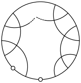
Figure 12. The standard form, where each of white vertices might not exist

Lemma 5.7.

If $g\geq k+3\geq 6$, the quotient $\mathfrak{a}_{g}(k)/\displaystyle\sum_{\begin{subarray}{c}i+j=k\\ i,j\geq 1\end{subarray}}[\mathfrak{a}_{g}(i),\mathfrak{a}_{g}(j)]$ is generated by spiders corresponding to chord diagrams of the standard form.

Proof.

It suffices to exhibit an algorithm by which a given chord diagram $C(S)$ corresponding to a spider $S$ is rewritten modulo brackets as a linear combination of chord diagrams of the standard form.

Suppose we are given a chord diagram $C$ corresponding to a spider with multiplicity $m(C)$. We may assume that $C$ is not separable.

If $C$ does not have a single paired chord, we take two adjacent vertices. By using the colors $i$, $j$ of these vertices, we can write $C=C(S(i,j,X))$ for some word $X$ of colors with length bigger than $2$. Then we have

$$S(i,j,X) =[S(X,n),\ S(-n,i,j)]$$

$$\quad+\sum_{\tiny\begin{subarray}{c}\mbox{color $-i$}\\ \mbox{in $X$}\end{subarray}}\pm S(n,Z_{1},j,-n,Z_{2})+\sum_{\tiny\begin{subarray}{c}\mbox{color $-j$}\\ \mbox{in $X$}\end{subarray}}\pm S(n,Z_{1},-n,i,Z_{2})$$

where $n>0$ and $-n$ are colors not possessed by $C$, and $Z_{1}$, $Z_{2}$ are some words. While the words $Z_{1}$, $Z_{2}$ differ in each term of the summation, precisely speaking, we use the same letters here for simplicity. In the right hand side, each of $S(n,Z_{1},j,-n,Z_{2})$ and $S(n,Z_{1},j,-n,Z_{2})$ has a single paired color $n$ and has multiplicity not bigger than $m(C)$.

Define a chord diagram $C$ having the configuration $\mathcal{F}_{l}$ ($l=1,2,\ldots)$ to be the one corresponding to a spider

$$S(c_{1},c_{2},-c_{1},c_{3},-c_{2},\ldots,c_{l},-c_{l-1},X,-c_{l},Y),$$

where colors $\pm c_{1},\pm c_{2},\ldots,\pm c_{l}$ are mutually distinct, and $X$, $Y$ are words (which might be empty) having no colors $\pm c_{1},\pm c_{2},\ldots,\pm c_{l}$. Diagrammatically, a chord diagram $C$ having the configuration $\mathcal{F}_{l}$ is given as in Figure 13. Now we inductively show that a chord diagram $C$ having the configuration $\mathcal{F}_{l}$ can be written as a linear combination of chord diagrams having the configuration $\mathcal{F}_{l+1}$ and having multiplicities not bigger than $m(C)$ modulo brackets unless it is already of the standard form.

Figure 13. The configuration $\mathcal{F}_{l}$

(The first step) By the argument in the third paragraph of this proof, we may assume that the chord diagram $C$ has at least one single paired chord colored by $\pm c_{1}$. Let $X$ and $Y$ be the regions separated by the single paired chord so that the diagram $C$ corresponds to the spider $S(c_{1},X,-c_{1},Y)$.

If $X$ or $Y$ has no vertices, then $C$ is separable and we are done.

If $X$ has at least two vertices, we have

$$S(c_{1},X,-c_{1},Y) =[S(c_{1},n,-c_{1},Y),\ S(-n,X)]$$

$$\quad+\sum_{\tiny\begin{subarray}{c}\mbox{pairing of}\\ \mbox{$X$ and $Y$}\end{subarray}}\pm S(c_{1},n,-c_{1},Z_{1},-n,Z_{2})$$

where $n>0$ and $-n$ are new colors as before (hereafter we omit these words about the new color $n$). Each of the spiders $S(c_{1},n,-c_{1},Z_{1},-n,Z_{2})$ has the configuration $\mathcal{F}_{2}$ with $c_{2}=n$ and multiplicity not bigger than $m(C)$.

If $X$ has only one vertex $v$, then $Y$ has at least two vertices since $k\geq 3$ and the diagram $C$ corresponds to the spider $S(c_{1},c_{v},-c_{1},Y)$, where $c_{v}$ is the color of $v$. In this case, there are three possibilities:

• If $v$ is unpaired, then it is separable.

• If $v$ is single paired, then $C$ has the configuration $\mathcal{F}_{2}$ with $c_{2}=c_{v}$.

• If $v$ is multiple paired, consider the equality

  $$S(c_{1},c_{v},-c_{1},Y) =[S(c_{1},c_{v},-c_{1},n),\ S(-n,Y)]$$

  $$\quad+\sum_{\tiny\begin{subarray}{c}\mbox{color $-c_{v}$}\\ \mbox{in $Y$}\end{subarray}}\pm S(-c_{1},n,c_{1},Z_{1},-n,Z_{2}).$$

  Each of the spiders $S(-c_{1},n,c_{1},Z_{1},-n,Z_{2})$ has the configuration $\mathcal{F}_{2}$ and multiplicity less than $m(C)$ since a pair of multiple paired vertices colored by $\pm c_{v}$ was exchanged for single paired vertices colored by $\pm n$.

In any case, we have checked that we can proceed to the next step.

(The inductive step) Suppose that any chord diagram having the configuration $\mathcal{F}_{i}$ $(i=1,2,3,\ldots,l-1)$ is written as a linear combination of chord diagrams having the configuration $\mathcal{F}_{i+1}$ and having multiplicities not bigger than $m(C)$. Let $C$ be a chord diagram having the configuration $\mathcal{F}_{l}$ as in Figure 12, where $X$ is the region between the vertices colored by $-c_{l-1}$ and $-c_{l}$ and $Y$ is the region between the vertices colored by $-c_{l}$ and $c_{1}$.

• Suppose that $X$ has no vertices. If $Y$ has at most one vertex, the diagram $C$ is of standard form. Otherwise, $Y$ has at least two vertices. Therefore $C$ is separable.

• Suppose that $X$ has at least two vertices. Then $C$ corresponds to the spider $S(c_{1},c_{2},-c_{1},c_{3},\ldots,c_{l},-c_{l-1},X,-c_{l},Y)$. Consider the equality

  $$S(c_{1},c_{2},-c_{1},c_{3},\ldots,c_{l},-c_{l-1},X,-c_{l},Y)$$

  $$=[S(c_{1},c_{2},-c_{1},c_{3},\ldots,c_{l},-c_{l-1},n,-c_{l},Y),S(-n,X)]$$

  $$\quad+\sum_{\tiny\begin{subarray}{c}\mbox{pairing of}\\ \mbox{$X$ and $Y$}\end{subarray}}\pm S(c_{1},c_{2},-c_{1},c_{3},\ldots,c_{l},-c_{l-1},n,-c_{l},Z_{1},-n,Z_{2}).$$

  Each of the spiders $S(c_{1},c_{2},-c_{1},c_{3},\ldots,c_{l},-c_{l-1},n,-c_{l},Z_{1},-n,Z_{2})$ has the configuration $\mathcal{F}_{l+1}$ and multiplicity not bigger than $m(C)$.

• Suppose that $X$ has only one vertex $v$. Let $c_{v}$ be the color of $v$.

  • Suppose that $v$ is unpaired. If $Y$ has at most one vertex, then $C$ is of standard form. Otherwise, $C$ is separable.

  • If $v$ is single paired, $C$ has the configuration of $\mathcal{F}_{l+1}$.

  • If $v$ is multiple paired, then $Y$ has at least two vertices. Consider the equality

    $$S(c_{1},c_{2},-c_{1},c_{3},\ldots,c_{l},-c_{l-1},c_{v},-c_{l},Y)$$

    $$=[S(c_{1},c_{2},-c_{1},c_{3},\ldots,c_{l},-c_{l-1},c_{v},-c_{l},n),S(-n,Y)]$$

    $$\quad+\sum_{\tiny\begin{subarray}{c}\mbox{color $-c_{v}$}\\ \mbox{in $Y$}\end{subarray}}\pm S(c_{1},c_{2},-c_{1},c_{3},\ldots,c_{l},-c_{l-1},Z_{1},-n,Z_{2},-c_{l},n).$$

    Each of the spiders $S(c_{1},c_{2},-c_{1},c_{3},\ldots,c_{l},-c_{l-1},Z_{1},-n,Z_{2},-c_{l},n)$ has the configuration $\mathcal{F}_{l-1}$, namely we have stepped backward. However their multiplicity are less than $m(C)$ since a pair of multiple paired vertices colored by $\pm c_{v}$ was exchanged for single paired vertices colored by $\pm n$. Hence in repeating this rewriting process, we meet this case at most $m(C)$ times and we can finally go to the next step.

Therefore the induction works and we finish the proof. ∎

Next we introduce chord slides for chord diagrams to show that any chord diagram of the standard form is in $\mathop{\mathrm{Im}}\nolimits[\,\cdot\,,\,\cdot\,]$. Hereafter we assume that all chord diagrams have no multiple paired vertices. Consider spiders having two adjacent vertices colored by $i$ and $j$, which might be negative. Suppose first that both $i$ and $j$ are single paired. Then we have the following equalities:

$$S(X,i,j,Y,-j,Z,-i) =\mathrm{sign}(n)[S(X,n,Y,-j,Z,-i),S(i,j,-n)]$$

$$\quad+\mathrm{sign}(ni)S(X,n,Y,-j,Z,j,-n)$$

$$\quad+\mathrm{sign}(nj)S(X,n,Y,-n,i,Z,-i),$$

$$S(X,i,j,Y,-i,Z,-j) =\mathrm{sign}(n)[S(X,n,Y,-i,Z,-j),S(i,j,-n)]$$

$$\quad+\mathrm{sign}(ni)S(X,n,Y,-i,Z,-n,i)$$

$$\quad+\mathrm{sign}(nj)S(X,n,Y,j,-n,Z,-j),$$

where $\mathrm{sign}(m)\in\{\pm 1\}$ denotes the sign of an integer $m\neq 0$. These equalities are diagrammatically expressed (up to sign) as in the first two equalities of Figure 14, which look like “chord slides to two directions”. Next suppose that $i$ is single paired and $j$ is unpaired. Then we have

$$S(X,i,j,Y,-i)=\mathrm{sign}(n)[S(X,n,Y,-i),S(i,j,-n)]+\mathrm{sign}(ni)S(X,n,Y,j,-n).$$

This equality is diagrammatically expressed (up to sign) as in the last equality of Figure 14. Note that in every case of the above, the color of the edge on which another chord slides changes after a chord slide.

Figure 14. Chord slides

In using chord slides, the following observation is easy but important. Let $\Sigma$ be a surface obtained from a chord diagram of the standard form with $l\geq 2$ single paired chords by fattening, where we ignore the crossings inside the outer circle. The boundary $\partial\Sigma$ of $\Sigma$ contains the outer circle and we call the other components of $\partial\Sigma$ the inner boundary.

Lemma 5.8.

The inner boundary of $\Sigma$ is connected if $l$ is even, and consists of two connected components if $l$ is odd.

Proof.

It is easy to see that the statement holds for $l=2$. Then we can inductively check that the statement holds for general cases by comparing the connection of the boundary before and after adding a new chord. ∎

Proof of Theorem 5.1 when $k\equiv 0\pmod{4}$.

There are two patterns of the standard form. The first one consists of two unpaired vertices and an even number of single paired chords. In this case, we can slide the unpaired vertices so that they are adjacent, which is possible because the inner boundary of the fattened surface is connected. Then the chord diagram becomes separable.

The second pattern consists of no unpaired vertex and an odd number of single paired chords. To treat this pattern, we consider a chord diagram having the configuration of the standard form with one more chord $l$ intersecting with the others at one point as in the left hand side of Figure 15. For such a diagram, we can move the intersecting point by a chord slide as shown in the same figure, where the second diagram of the right hand side is separable.

Figure 15. Sliding the intersection

Now take a chord diagram of the standard form consisting of $(k+2)/2$ chords as in the left hand side of Figure 16. We may consider it to be a diagram of the standard form consisting of $k/2$ chords with one more chord colored by $\pm c_{1}$. To this diagram, we apply the chord slide discussed above with regarding the chord colored by $\pm c_{1}$ as $l$. By iterating chord slides, we get to the chord diagram of the right hand side of Figure 16, which is shown to be in $\mathop{\mathrm{Im}}\nolimits[\,\cdot\,,\,\cdot\,]$ by considering the result of the chord slide at $\ast$ (see also the first line of Figure 17). ∎

Figure 16. The right hand side is the final stage of a chord cycling

Hereafter we call the operation used in the second pattern of the above (i.e. moving the chord colored by $\pm c_{1}$ from right to left) a chord cycling.

Figure 17. Chord cyclings for odd and even numbers of chords

Proof of Theorem 5.1 when $k\equiv 1\pmod{4}$.

In this case, the standard form consists of a unique unpaired vertex and an odd number of single paired chords. Then by a chord cycling with ignoring the unpaired vertex, we can slide the diagram to a separable one. ∎

In the remaining two cases, we can apply the same argument as above only to chord diagrams of the standard form consisting of two unpaired vertices and an odd number of single paired chords, when $k\equiv 2\pmod{4}$. Therefore we can finish the proof of Theorem 5.1 by considering the following two types of chord diagrams (see Figure 18):

• chord diagrams of the standard form consisting of no unpaired vertices and $(2l+2)$ single paired chords, where $k=4l+2$,

• chord diagrams of the standard form consisting of one unpaired vertex and $(2l+2)$ single paired chords, where $k=4l+3$.

  

  Figure 18. Type (a) and Type (b)

For each of them, a chord cycling results to another chord diagram of the standard form with distinct colors (see the second line of Figure 17).

Lemma 5.9.

Under the assumption $g\geq k+3\geq 6$, we have the following.

$(1)$ Every chord diagram of Type $\mathrm{(a)}$ shown in the left of Figure 18 is transformed up to sign to the one with $c_{i}=i$ for $i=1,2,\ldots,2l+2$ by chord slides.

$(2)$ Let $C$ be a chord diagram of Type $\mathrm{(b)}$ whose unique unpaired vertex is colored by $c$ as shown in the right of Figure 18. Then for any fixed colors $\{d_{1},d_{2},\ldots,d_{2l+2}\}$ consisting of mutually distinct positive integers and not including $\pm c$, the diagram $C$ is transformed up to sign to the one with $c_{i}=d_{i}$ for $i=1,2,\ldots,2l+2$ by chord slides.

Proof.

(1) Let $C$ be a chord diagram of Type (a) as in the left of Figure 18. We associate this diagram with the sequence $[c_{1},c_{2},\ldots,c_{2l+2}]$ of colors.

By the assumption $g\geq 4l+5$, we have

$$\{1,2,\ldots,g\}-\{1,2,\ldots,2l+2,|c_{1}|,|c_{2}|,\ldots,|c_{2l+2}|\}\neq\emptyset.$$

This means that every time we apply a chord slide, we can choose an integer from this set as a new color, namely the integer $n$ of the formulas in Figure 14. Taking account of this observation we can apply a chord cycling to $C$ so that the resulting chord diagram of the standard form is associated with the sequence

$$[c_{2},n_{3},c_{4},n_{5},\ldots,n_{2l+1},c_{2l+2},c_{1}]$$

where $n_{3},n_{5},\ldots,n_{2l+1}\in\{1,2,\ldots,g\}-\{1,2,\ldots,2l+2\}$. By iterating chord cyclings, we obtain chord diagrams of the standard form associated with the sequences

$$\qquad\,[c_{2},n_{3},c_{4},n_{5},\ldots,n_{2l+1},c_{2l+2},c_{1}]$$

$$\longrightarrow[n_{3},n_{4},n_{5},\ldots,n_{2l+1},n_{2l+2},c_{1},c_{2}]$$

$$\longrightarrow[n_{4},n^{\prime}_{5},\ldots,n^{\prime}_{2l+1},n_{2l+2},n_{1},c_{2},n_{3}]$$

$$\longrightarrow[n^{\prime}_{5},n^{\prime}_{6},\ldots,n^{\prime}_{2l+1},n^{\prime}_{2l+2},n_{1},n_{2},n_{3},n_{4}]$$

$$\longrightarrow[n^{\prime}_{6},2l+1,n^{\prime}_{8},n^{\prime\prime}_{9},\ldots,n^{\prime\prime}_{2l+1},n^{\prime}_{2l+2},n^{\prime\prime}_{1},n_{2},n^{\prime\prime}_{3},n_{4},n^{\prime}_{5}]$$

$$\longrightarrow[2l+1,2l+2,n^{\prime\prime}_{9},n^{\prime\prime}_{10},\ldots,n^{\prime\prime}_{2l+1},n^{\prime\prime}_{2l+2},n^{\prime\prime}_{1},n^{\prime\prime}_{2},n^{\prime\prime}_{3},n^{\prime\prime}_{4},n^{\prime}_{5},n^{\prime}_{6}]$$

$$\longrightarrow[2l+2,1,n^{\prime\prime}_{10},3,n^{\prime\prime}_{12},5,\ldots,2l-4,n^{\prime\prime}_{2l+2},2l-3,n^{\prime\prime}_{2},2l-2,n^{\prime\prime}_{4},2l-1,n^{\prime}_{6},2l+1]$$

$$\longrightarrow[1,2,3,\ldots,2l+1,2l+2]$$

where the positive integers $n_{i}$, $n^{\prime}_{j}$, $n^{\prime\prime}_{k}$ are taken from $\{1,2,\ldots,g\}-\{1,2,\ldots,2l+2\}$. Our claim follows from this. Note that the above argument works also for small $l$.

(2) Take a chord diagram of Type (b) shown in the right of Figure 18. Since the inner boundary is connected, we can slide the unique unpaired vertex along all chords so that the colors of the other vertices are changed as indicated. This is possible because the assumption $g\geq 4l+6$ implies that

$$\{1,2,\ldots,g\}-\{|c|,|c_{1}|,|c_{2}|,\ldots,|c_{2l+2}|,|d_{1}|,|d_{2}|,\ldots,|d_{2l+2}|\}\neq\emptyset,$$

which enables us to use an argument similar to (1). ∎

To show that the chord diagrams specialized in Lemma 5.9 are in $\mathop{\mathrm{Im}}\nolimits[\,\cdot\,,\,\cdot\,]$, we use the following mirror image argument. For a spider $S$, we define its mirror $S^{m}$ as the spider obtained from $S$ by sorting its legs in reverse order. In terms of chord diagrams, the chord diagram $C(S^{m})$ is obtained from $C(S)$ by taking its mirror image. The following lemma is easily checked.

Lemma 5.10.

For spiders $S_{1}$ and $S_{2}$, their bracket $[S_{1}^{m},S_{2}^{m}]$ is obtained from $[S_{1},S_{2}]$ by taking the mirror for each spider in it.

Proof of Theorem 5.1 when $k\equiv 2\pmod{4}$.

There are two patterns of the standard form. The first one consists of two unpaired vertices and an odd number of single paired chords. In this case, we can use chord cyclings with ignoring the unpaired vertices to show that the chord diagram is in $\mathop{\mathrm{Im}}\nolimits[\,\cdot\,,\,\cdot\,]$ as in the cases where $k\equiv 0,1\pmod{4}$.

The second one is of Type (a), where $k=4l+2$. By Lemma 5.9, it suffices to show that the spider

$$\widetilde{S}=S(1,2,-1,3,-2,4,\ldots,-2l,2l+2,-(2l+1),-(2l+2))$$

is in $\mathop{\mathrm{Im}}\nolimits[\,\cdot\,,\,\cdot\,]$. For that, we “divide” the corresponding chord diagram at the center of the chain of chords. That is, we consider the equality

$$\widetilde{S} =[S(1,2,\ldots,\underline{l+1},-l,\underline{l+2},n),\ S(-n,\underline{-(l+1)},l+3,\underline{-(l+2)},\ldots,-(2l+2))]$$

$$\quad-S(1,2,\ldots,-(l-1),\underline{l+3,-(l+2),l+4,\ldots,-(2l+1),-(2l+2),-n},-l,l+2,n)$$

$$\quad-S(-n,-(l+1),l+3,\underline{n,1,2,\ldots,l+1,-l},l+4,\ldots,-(2l+1),-(2l+2)).$$

Here we remark that the third term of the right hand side is obtained up to sign from the second term by taking its mirror and applying the symplectic action

$$a_{i}\longmapsto-b_{2l+3-i},\quad b_{i}\longmapsto a_{2l+3-i}\quad(i=1,2,\ldots,2l+2),$$

$$a_{n}\longmapsto-b_{n},\quad b_{n}\longmapsto a_{n}.$$

We use Lemma 5.7 to rewrite the second term as the linear combination $P$ of chord diagrams of the standard form. As for the third term, Lemma 5.10 and the fact that the bracket operation is equivariant with respect to the symplectic action show that we can rewrite it as the linear combination $Q$ obtained from $P$ by taking the mirror and applying the symplectic action to each chord diagram. It follows from Lemma 5.9 that the sum $P+Q$ is rewritten as $2m\widetilde{S}$ by some even number $2m$. Therefore we have $\widetilde{S}\equiv 2m\widetilde{S}$, which implies that $\widetilde{S}\equiv 0$ in $H_{1}(\mathfrak{a}_{g}^{+})$. ∎

Proof of Theorem 5.1 when $k\equiv 3\pmod{4}$.

The standard form consists of a unique unpaired vertex and $(2l+2)$ single paired chords, where $k=4l+3$. By Lemma 5.9, it suffices to show that the spider

$$S(c,d_{1},d_{2},-d_{1},d_{3},-d_{2},d_{4},\ldots,-d_{2l},d_{2l+2},-d_{2l+1},-d_{2l+2})$$

is in $\mathop{\mathrm{Im}}\nolimits[\,\cdot\,,\,\cdot\,]$. For that, we can use almost the same argument as the case where $k\equiv 2\pmod{4}$ by ignoring the unique unpaired vertex. Note that the algorithm of Lemma 5.7 keeps the color $c$ of the unpaired vertex. ∎

Proof of Theorem 1.1 $\mathrm{(iii)}$.

If we apply the last split exact sequence in Section 2 to the present case, we have

$$H_{1}(\mathfrak{a}_{g})\cong H_{1}(\mathfrak{a}_{g}^{+})_{\mathfrak{sp}}\oplus H_{1}(\mathfrak{a}_{g}(0))=H_{1}(\mathfrak{a}_{g}^{+})_{\mathfrak{sp}}\oplus H_{1}(\mathfrak{sp}(2g,{\mathbb{Q}})).$$

As is well-known that $H_{1}(\mathfrak{sp}(2g,{\mathbb{Q}}))=0$. Hence after taking the limit, we obtain

$$\lim_{g\to\infty}H_{1}(\mathfrak{a}_{g})\cong\lim_{g\to\infty}H_{1}(\mathfrak{a}_{g}^{+})_{\mathfrak{sp}}.$$

Now the first author’s computation [18, Theorem 6] and Theorem 5.1 show that

$$\lim_{g\to\infty}H_{1}(\mathfrak{a}_{g}^{+})_{\mathfrak{sp}} \cong\lim_{g\to\infty}(\mathfrak{a}_{g}(1)\oplus(\wedge^{2}H_{\mathbb{Q}}/\langle\omega_{0}\rangle))_{\mathfrak{sp}}$$

$$\cong\lim_{g\to\infty}(S^{3}H_{\mathbb{Q}}\oplus\wedge^{3}H_{\mathbb{Q}}\oplus(\wedge^{2}H_{\mathbb{Q}}/\langle\omega_{0}\rangle))_{\mathfrak{sp}}=0.$$

This completes the proof. ∎

6. Application to cohomology of moduli spaces of curves

In this section, we apply one of our main theorems, Theorem 1.1, to obtain a new proof of the vanishing theorem of Harer (Theorem 1.4). First we recall the following foundational result of Harer.

Theorem 6.1 (Harer [9]).

The virtual cohomological dimension of $\mathcal{M}_{g}^{m}$ is given by

$$\mathrm{vcd}\,\mathcal{M}_{g}^{m}=\begin{cases}4g-5&(g\geq 2,m=0)\\ 4g-4+m&(g>0,m>0)\\ m-3&(g=0)\end{cases}$$

so that the rational cohomology group

$$H^{k}(\mathbf{M}_{g}^{m};\mathbb{Q})\cong H^{k}(\mathcal{M}_{g}^{m};\mathbb{Q})$$

vanishes for any $k>\mathrm{vcd}\,\mathcal{M}_{g}^{m}$.

Here we denote by $\mathcal{M}_{g}^{m}$ the mapping class group of $\Sigma_{g}$ with $m$ distinct marked points and by $\mathbf{M}_{g}^{m}$ the moduli space of curves of genus $g$ with $m$ distinct marked points. As is well known, there exists a canonical isomorphism

$$H^{*}(\mathbf{M}_{g}^{m};\mathbb{Q})\cong H^{*}(\mathcal{M}_{g}^{m};\mathbb{Q})\quad(2g-2+m>0).$$

Now we prove the following result which gives an alternative proof of the theorem of Harer mentioned above.

Theorem 6.2.

For any $g\geq 2$, the top degree rational cohomology group of the moduli space $\mathbf{M}_{g}^{m}\ (m=0,1)$ as well as the mapping class group $\mathcal{M}_{g}^{m}\ (m=0,1)$, with respect to its virtual cohomological dimension, vanishes. More precisely, we have

$$H^{4g-5}(\mathbf{M}_{g};\mathbb{Q})\cong H^{4g-5}(\mathcal{M}_{g};\mathbb{Q})=0$$

$$H^{4g-3}(\mathbf{M}_{g}^{1};\mathbb{Q})\cong H^{4g-3}(\mathcal{M}_{g}^{1};\mathbb{Q})=0$$

for any $g\geq 2$.

To prove Theorem 6.2, we recall the following theorem of Kontsevich which is the associative version of the three types of graph (co)homologies he presented in [14, 15].

Theorem 6.3 (Kontsevich [14, 15]).

For $n\geq 1$, there exists an isomorphism

$$PH_{k}\big{(}\lim_{g\to\infty}\mathfrak{a}_{g}\big{)}_{2n}\cong\bigoplus_{\begin{subarray}{c}2g-2+m=n\\ m>0\end{subarray}}H^{2n-k}(\mathbf{M}_{g}^{m};\mathbb{Q})^{\mathfrak{S}_{m}}.$$

Proof of Theorem 6.2.

First we prove the vanishing $H^{4g-3}(\mathcal{M}_{g}^{1};\mathbb{Q})=0$ for any $g\geq 1$. By Theorem 1.1, we know that $\lim_{g\to\infty}H_{1}(\mathfrak{a}_{g})_{2n}=0$ for any $n$. If we substitute this in Theorem 6.3, then we obtain

$$H^{4g-5+2m}(\mathcal{M}_{g}^{m};\mathbb{Q})^{\mathfrak{S}_{m}}=0\quad\text{for any $m\geq 1$}.$$

If we put $m=1$, then we can conclude that

$$H^{4g-3}(\mathcal{M}_{g}^{1};\mathbb{Q})=0\quad\text{for any $g\geq 1$}.$$

Next, we deduce $H^{4g-5}(\mathcal{M}_{g};\mathbb{Q})=0\ (g\geq 2)$ from the above. For this, consider the group extension

$$1\longrightarrow\pi_{1}\Sigma_{g}\longrightarrow\mathcal{M}_{g}^{1}\longrightarrow\mathcal{M}_{g}\longrightarrow 1\quad(g\geq 2)$$

and let $\{E^{p,q}_{r},d^{p,q}_{r}\}$ denote the spectral sequence associated to the above extension for the rational cohomology group. We have $E^{p,q}_{2}\cong H^{p}(\mathcal{M}_{g};H^{q}(\pi_{1}\Sigma_{g};\mathbb{Q}))$. As is well known, there exists a natural isomorphism $H^{q}(\pi_{1}\Sigma_{g};\mathbb{Q})\cong H^{q}(\Sigma_{g};\mathbb{Q})$ and, by Theorem 6.1, $H^{p}(\mathcal{M}_{g};\mathcal{H})=0$ for any $p>4g-5$ and for any rational twisted coefficients $\mathcal{H}$. It follows that the only $E_{2}$-term, in total degree $p+q=4g-3$, which may survive in the $E_{\infty}$ term is $E^{4g-5,2}_{2}\cong H^{4g-5}(\mathcal{M}_{g};\mathbb{Q})$. On the other hand, it is easy to see that

$$E_{2}^{4g-5,2}\cong E_{3}^{4g-5,2}\cong\cdots\cong E_{\infty}^{4g-5,2}=H^{4g-3}(\mathcal{M}_{g}^{1};\mathbb{Q})=0.$$

This is a special case of the fact, proved in [16], that the above spectral sequence collapses at the $E_{2}$-term. We can now conclude that $H^{4g-5}(\mathcal{M}_{g};\mathbb{Q})=0$ as required. ∎

Remark 6.4.

In contrast with the above result, the situation in the cases of genus $0$ and $1$ is completely different. According to Getzler [7], the rational cohomology group of top degree $H^{m-3}(\mathbf{M}_{0}^{m};\mathbb{Q})$ has dimension $(m-2)!$. In [8], Getzler also determined the $\mathfrak{S}_{m}$-equivariant Serre characteristic for $\mathbf{M}_{1}^{m}$. In particular, the top degree $\mathfrak{S}_{m}$-invariant rational cohomology group $H^{m}(\mathbf{M}_{1}^{m};\mathbb{Q})^{\mathfrak{S}_{m}}$ is highly non-trivial for infinitely many $m$.

In [18], the first author determined the weight $2$ part $H_{1}(\mathfrak{a}_{g}^{+})_{2}$ of the abelianization of $\mathfrak{a}_{g}^{+}$ and by applying the theorem of Kontsevich cited above (Theorem 6.3), he constructed a series of cohomology classes in $H^{4m+1}(\mathbf{M}_{1}^{4m+1})^{\mathfrak{S}_{4m+1}}$ for $m=1,2,\ldots$. Then Conant [2] proved that these classes are all non-trivial. It would be an interesting problem to seek for possible special property of these classes among the whole classes which Getzler determined.

7. Concluding remarks

In this section, we make a few remarks concerning the ingredients of this paper.

Remark 7.1.

We have been investigating not only the first homology groups of Lie algebras $\mathfrak{a}_{g}$ and $\mathfrak{h}_{g,1}$ but also higher homology groups as well. In particular, we had already a glimpse of considerable difference between the structures of $H_{2}(\mathfrak{a}_{g})$ and $H_{2}(\mathfrak{h}_{g,1})$. We will discuss this in a forthcoming paper.

Remark 7.2.

The Lie algebra $\mathfrak{a}_{g}$ appeared in a recent work of Enomoto and Satoh [6] and also in Kawazumi and Kuno [13], where they found certain new roles of this Lie algebra. We refer to the above cited papers for details.

References

[1]
T. Church, B. Farb, A. Putman,
The rational cohomology of the mapping class group vanishes in its virtual cohomological dimension,
Int. Math. Res. Not. 21 (2012), 5025–5030.
[2]
J. Conant,
Ornate necklaces and the homology of the genus one mapping class group,
Bull. London. Math. Soc. 39 (2007) 881–891.
[3]
J. Conant, M. Kassabov, K. Vogtmann,
Hairy graphs and the unstable homology of
, and ,
preprint,
arXiv:1107.4839v2 [math.AT].
[4]
J. Conant, K. Vogtmann,
On a theorem of Kontsevich,
Algebr. Geom. Topol. 3 (2003) 1167–1224.
[5]
M. Culler, K. Vogtmann,
Moduli of graphs and automorphisms of free groups,
Invent. Math. 84 (1986) 91–119.
[6]
N. Enomoto, T. Satoh,
New series in the Johnson cokernels of the mapping class groups of surfaces,
preprint,
arXiv:1012.2175v3 [math.RT].
[7]
E. Getzler,
Operads and moduli spaces of genus Riemann surfaces, In “The moduli space of curves”,
Progr. Math. 129 (1995) 199–230.
[8]
E. Getzler,
Resolving mixed Hodge modules on configuration spaces,
Duke Math. J. 96 (1999) 175–203.
[9]
J. Harer,