X-ray properties expected from AGN feedback in elliptical galaxies

Abstract

The evolution of the interstellar medium (ISM) of elliptical galaxies experiencing feedback from accretion onto a central supermassive black hole has been studied recently with high-resolution 1D hydrodynamical simulations; these included cooling, heating and radiative pressure effects on the gas, specific for an average AGN spectral energy distribution, a RIAF-like radiative efficiency, mechanical energy, mass and momentum input from AGN winds, and the effects of starbursts associated with accretion. Here we focus on the observational properties of the models in the soft and hard X-ray bands, specifically on 1) the nuclear X-ray luminosity; 2) the global X-ray luminosity and temperature of the hot ISM; 3) its temperature and X-ray brightness profiles, during quiescence, and before, during and after an outburst. After an evolution of $\sim 10$ Gyr, the bolometric nuclear emission is very sub-Eddington ($l\sim 10^{-4}$), and within the range observed, though larger than the most frequently observed values. The nuclear bursts last for $\approx 10^{7}$ yrs, and the duty-cycle of nuclear activity is a few$\times(10^{-3}-10^{-2})$, when calculated over the last 6 Gyr. The ISM thermal luminosity $L_{\rm X}$ oscillates in phase with the nuclear one, but drawing much broader peaks; a comparison with observed $L_{\rm X}$ values, for galaxies of optical luminosity similar to that of the models, shows that this behavior helps reproduce statistically the observed large $L_{\rm X}$ variation. At the present epoch, the largest observed $L_{\rm X}$ could be reproduced only by adding an external confining medium. The average gas temperature is within the observed range; when limited to within $R_{\rm e}$, its values lie on the upper half of those observed. In quiescence, the temperature profile has a negative gradient; thanks to past outbursts, the brightness profile lacks the steep shape typical of inflowing models. After outbursts, disturbances are predicted in the temperature and brightness profiles (as analyzed also with the unsharp masking). Most significantly, during major accretion episodes, a hot bubble from shocked hot gas is inflated at the galaxy center (within $\approx 100$ pc); the bubble would be conical in shape, in real galaxies, and show radio emission. Its detection in the X-rays is within current capabilities, though it would likely remain unresolved. The ISM resumes its smooth appearance on a time-scale of $\approx 200$ Myr; the duty-cycle of perturbances in the ISM is of the order of 5-10%. The present analysis reveals an agreement of the models with the observations, but also evidences that additional input physics is important in the ISM-black hole coevolution, to fully account for the properties of real galaxies. The main insertions to the models would be a confining external medium and a jet. The jet will reduce further the mass available for accretion (and then $l$), and may help, together with an external pressure, to produce flat or positive temperature gradient profiles (that are common among galaxies in high density environments). Alternatively to the jet, a reduction of $l$ can be obtained if the switch from high to low radiative efficiency takes place at a larger $l$ ($\simeq 0.1$) than routinely assumed ($\simeq 0.01$).

1 Introduction

Supermassive black holes (MBHs) at the centers of bulges and elliptical galaxies play an important role in the processes of galaxy formation and evolution (e.g., Cattaneo et al. 2009), as testified by remarkable correlations between host galaxy properties and the MBH masses (e.g., Magorrian et al. 1998, Ferrarese & Merritt 2000, Gebhardt et al. 2000, Graham et al. 2001) and as supported by many theoretical studies (e.g., Silk & Rees 1998, Haiman, Ciotti & Ostriker 2004; Merloni et al. 2004, Sazonov et al. 2005, Di Matteo, Springel & Hernquist 2005, Hopkins et al. 2006, Somerville et al. 2008, Kormendy et al. 2009). An important aspect of the coevolution process is the radiative and mechanical feedback by the accreting MBH onto the galactic interstellar mediun (ISM) that is continuously replenished by normal stellar mass losses, at a rate of the order of $\approx 1M_{\odot}$ yr^-1 in a medium-mass galaxy. In absence of feedback from a central MBH (and stripping from the intracluster medium in case of satellite galaxies), this ISM would develop a flow directed towards the galactic center, accreting ${\mathrel{\mathchoice{\lower 2.9pt\vbox{\halign{$\m@th\displaystyle\hfil#\hfil$\cr>\crcr\sim\crcr}}}{\lower 2.9pt\vbox{\halign{$\m@th\textstyle\hfil#\hfil$\cr>\crcr\sim\crcr}}}{\lower 2.9pt\vbox{\halign{$\m@th\scriptstyle\hfil#\hfil$\cr>\crcr\sim\crcr}}}{\lower 2.9pt\vbox{\halign{$\m@th\scriptscriptstyle\hfil#\hfil$\cr>\crcr\sim\crcr}}}}}1M_{\odot}$ yr^-1 in a process similar to a “cooling flow”. Instead, in low mass galaxies, type Ia supernova (SNIa) heating is able to sustain a low-luminosity, global galactic wind (e.g., Ciotti et al. 1991, David et al. 1991, Pellegrini & Ciotti 1998), and the central MBH is in a state of permanent, highly sub-Eddington hot accretion (Ciotti & Ostriker 2011).

Therefore, in medium to high mass galaxies, feedback is required by the following empirical arguments: 1) the large amount of gas lost by the passively evolving stellar population during the galaxies’ lifetime is not observed (e.g., Peterson & Fabian 2006), and just ${\mathrel{\mathchoice{\lower 2.9pt\vbox{\halign{$\m@th\displaystyle\hfil#\hfil$\cr<\crcr\sim\crcr}}}{\lower 2.9pt\vbox{\halign{$\m@th\textstyle\hfil#\hfil$\cr<\crcr\sim\crcr}}}{\lower 2.9pt\vbox{\halign{$\m@th\scriptstyle\hfil#\hfil$\cr<\crcr\sim\crcr}}}{\lower 2.9pt\vbox{\halign{$\m@th\scriptscriptstyle\hfil#\hfil$\cr<\crcr\sim\crcr}}}}}$1% of the mass made available by stars is contained in the masses of present epoch MBHs; 2) bright AGNs, as would be expected given the predicted mass accretion rate, are not commonly seen in the spheroids of the local Universe (e.g., Fabian & Canizares 1988, Pellegrini 2005). Thus AGN feedback is required just on the basis of a mass balance argument. Since over a large part of the galaxies extent, and for a large fraction of their lifetime, the ISM cooling time $t_{cool}$ is much lower than the galaxy age, one early quasar phase cannot be the solution to the cooling flow problem. The solution requires either steady heating, or heating with bursts on a timescale $\Delta t\approx t_{cool}$. Unfortunately, on a purely theoretical ground, how much radiative and mechanical energy and momentum output from the MBH can effectively interact with the surrounding ISM, and what are the resultant MBH masses, is difficult to establish.

Recently, the interaction of the MBH output with the inflowing gas has been studied with high-resolution 1D hydrodynamical simulations in a series of papers (Ciotti & Ostriker 2007; Ciotti, Ostriker & Proga 2009, 2010 hereafter Papers I and III; Shin, Ostriker & Ciotti 2010a,b; Ostriker et al. 2010; Jiang et al. 2010), that are currently being extended to 2D treatments (Novak, Ostriker & Ciotti 2010). These simulations implement a physically based detailed treatment of the radiative energy and momentum input from the MBH into the ISM, consistent both with observed average AGN spectra and theoretical calculations of radiation transport; they also include starformation, and a modelling of the mechanical energy and momentum feedback from AGN winds. The combined effects of radiative and mechanical feedback produce recurrent AGN burst phases accompanied by starformation, spaced apart by longer phases of relative quiescence. A cycle repeats with the galaxy seen alternately as an AGN/starburst for a small fraction of the time, and as a “normal” elliptical for much longer intervals. Accretion fueled feedback thus proves effective in suppressing long lasting cooling flows and in maintaining MBH masses within the range observed today, since the gas is mostly lost in outflows or consumed in starbursts. Remarkably, while star formation is suppressed when the AGN is in the low-luminosity state, it is enhanced by the strong AGN outbursts, consistent with observations (Schawinski et al. 2009). Note finally that a major role in producing global degassing, and in regulating the flow evolution, is also played by the SNIa’s heating.

The previous papers, with the exception of Pellegrini, Ciotti & Ostriker (2009), were mainly dedicated to the study of the accretion physics and the feedback effects. Here instead we focus on the appearance that the models would have if observed in the X-ray band, both in quiescence and during an outburst of activity. We concentrate on two models (named B2${}_{02}\,$and B3${}_{02}\,$) extracted from the suite of cases presented in Paper III (Table 1 therein), characterized by a mechanical feedback efficiency dependent on the Eddington scaled accretion luminosity. B2${}_{02}\,$and B3${}_{02}\,$were considered particularly successful, since their input parameters agree with previous theoretical studies or observations (as, e.g., for the AGN wind opening angle, and the peak value of mechanical efficiency, that are in accord with those estimated from 2D and 3D numerical simulations; Proga, Stone & Kallman 2000, Proga & Kallman 2004, Benson & Babul 2009), and, at the same time, their final properties (as mass fraction of a younger stellar population, MBH mass, etc.) are in reasonable accord with observations. The only difference in the input physics of B2${}_{02}\,$and B3${}_{02}\,$is the maximum value of the mechanical efficiency. Since in the simulations the treatment of feedback is physically based, not tuned to reproduce observations, any agreement or discrepancy of the resulting model properties with X-ray observations is relevant to improving our understanding of the MBH-ISM coevolution, putting further constraints on the input ingredients, and possibly telling us what additional physics may be important in the problem. However, we stress that the models describe an isolated galaxy, where ram-pressure stripping (in case of satellite galaxies) and intracluster medium pressure confinement (in case of group or cluster central galaxies) are not taken into account (see Shin et al. 2010b).

The main observational signatures investigated here include the nuclear and gaseous emissions, and the ISM temperature and brightness profiles in the quiescent phases, and before, during, after a burst. Particular attention is paid to the appearance and detectability of central hot bubbles, with diameters of $\sim$a hundred parsecs, that are produced by the models during outbursts, and to various kinds of disturbances in the hot ISM. The analysis is performed in the soft and hard X-ray bands, also after unsharp-masking. These predictions are relevant for their observational consequences, since the high angular resolution of the $Chandra$ satellite has allowed us to obtain the best definition ever for the hot gas properties of the galaxies of the local universe, by separating the contributions of stellar sources and hot gas, and the emission coming from different spatial regions within galaxies (e.g., Fabbiano 2011). In particular, in several elliptical galaxies various kinds of hot gas disturbances have been detected, likely resultant from nuclear activity (e.g., Finoguenov & Jones 2001, Jones et al. 2002, Forman et al. 2005, Machacek et al. 2006, O’Sullivan et al. 2007, Million et al. 2010). At the same time, nuclear emission values have been detected down to very low luminosities, comparable to those of X-ray binaries (e.g., Loewenstein et al. 2001, Gallo et al. 2010, Pellegrini 2010).

The paper is organized as follows. Section 2 summarizes the main evolutionary phases of the representative models (B3${}_{02}\,$and B3${}_{02}\,$) considered; Section 3 describes how the observational properties of the models are derived; Section 4 presents a comparison of the nuclear luminosities with existing observations; Section 5 discusses the evolution of the X-ray luminosity and emission-weighted temperature of the ISM; Section 6 presents the projected temperature and surface brightness profiles at representative times during quiescence and a nuclear outburst. Finally, in Section 7 we summarize and discuss the main results.

2 Two representative models: main features

The basic ideas behind the present class of models for feedback modulated accretion flows have been introduced in Ciotti & Ostriker (1997, 2001), and Ostriker & Ciotti (2005), and developed in detail in the papers listed in the Introduction; a comprehensive recent discussion is given in Ciotti & Ostriker (2011). Here we focus on models B2${}_{02}\,$and B3${}_{02}\,$from Paper III (where the description of the numerical code and the input physics is given). The initial parameter values and the main final properties of the models are given in Table 1.

The two models refer to an isolated elliptical galaxy placed on the Fundamental Plane, with a projected central stellar velocity dispersion $\sigma=260$ km s^-1, a total B-band luminosity $L_{\rm B}=5\times 10^{10}L_{\rm B\odot}$, and an effective radius $R_{\rm e}=6.9$ kpc. The stellar density profile is described by a Jaffe (1983) law, and the dark halo profile is such that the total (stellar+dark) mass density profile scales as $\rho\propto r^{-2}$ at large radii; all relevant dynamical properties used in the code are discussed in Ciotti, Morganti & de Zeeuw (2009). The dark-to-visible mass ratio is one within $R_{\rm e}$, and the resulting stellar mass-to-light ratio is $M_{*}/L_{\rm B}=5.8$. Finally, a standard SNIa’s rate declining with time $t$ as $t^{-1.1}$ is assumed. The initial MBH mass is set to $10^{-3}$ the initial stellar mass $M_{*}$, i.e., it is $2.9\times 10^{8}M_{\odot}$. The simulations begin at a galaxy age of $\sim 2$ Gyr (that is a redshift $z\sim 2$, the exact value depending on the epoch of elliptical galaxy formation, usually put at $z{\mathrel{\mathchoice{\lower 2.9pt\vbox{\halign{$\m@th\displaystyle\hfil#\hfil$\cr>\crcr\sim\crcr}}}{\lower 2.9pt\vbox{\halign{$\m@th\textstyle\hfil#\hfil$\cr>\crcr\sim\crcr}}}{\lower 2.9pt\vbox{\halign{$\m@th\scriptstyle\hfil#\hfil$\cr>\crcr\sim\crcr}}}{\lower 2.9pt\vbox{\halign{$\m@th\scriptscriptstyle\hfil#\hfil$\cr>\crcr\sim\crcr}}}}}2$).

The efficiency for producing radiation (Soltan 1982, Yu & Tremaine 2002) of material accreting on the MBH at the rate $\dot{M}_{\rm BH}$ is

$$\epsilon=0.2\times{A\dot{m}\over 1+A\dot{m}},$$ (1)

where $\dot{m}=\dot{M}_{\rm BH}/\dot{M}_{\rm Edd}$ is the Eddington-scaled accretion rate. Thus, for $A=100$, one has $\epsilon\sim 0.2$ at large mass accretion rates $\dot{m}\gg 0.01$, and $\epsilon$ declining as for radiatively inefficient accretion flows (RIAFs, Narayan & Yi 1994), as $\epsilon\sim 20\dot{m}$, for $\dot{m}{\mathrel{\mathchoice{\lower 2.9pt\vbox{\halign{$\m@th\displaystyle\hfil#\hfil$\cr<\crcr\sim\crcr}}}{\lower 2.9pt\vbox{\halign{$\m@th\textstyle\hfil#\hfil$\cr<\crcr\sim\crcr}}}{\lower 2.9pt\vbox{\halign{$\m@th\scriptstyle\hfil#\hfil$\cr<\crcr\sim\crcr}}}{\lower 2.9pt\vbox{\halign{$\m@th\scriptscriptstyle\hfil#\hfil$\cr<\crcr\sim\crcr}}}}}0.01$ (see also Sect. 4 for additional comments on this choice). The mechanical feedback implemented is that of the Broad Line Region winds (leading to outflow velocities of $\simeq 10^{4}$ km/s, similar to what observed, e.g. Chartas et al. 2003, Crenshaw et al. 2003), and reproduces the main features of the numerical modeling by Proga (2003). In particular, the mechanical efficiency scales with the Eddington ratio $l=L_{\rm BH}/L_{\rm Edd}$ (where $L_{\rm BH}=\epsilon\dot{M}_{\rm BH}c^{2}$ is the instantaneous bolometric accretion luminosity), reaching a maximum value $\epsilon_{\rm w}^{\rm M}$ of $3\times 10^{-4}$ (for B3${}_{02}\,$), and $10^{-3}$ (for B2${}_{02}\,$), when $l{\mathrel{\mathchoice{\lower 2.9pt\vbox{\halign{$\m@th\displaystyle\hfil#\hfil$\cr>\crcr\sim\crcr}}}{\lower 2.9pt\vbox{\halign{$\m@th\textstyle\hfil#\hfil$\cr>\crcr\sim\crcr}}}{\lower 2.9pt\vbox{\halign{$\m@th\scriptstyle\hfil#\hfil$\cr>\crcr\sim\crcr}}}{\lower 2.9pt\vbox{\halign{$\m@th\scriptscriptstyle\hfil#\hfil$\cr>\crcr\sim\crcr}}}}}2$; also, the aperture solid angle of the conical nuclear wind increases at increasing $l$. Note that the values of the mechanical efficiency in cols. (2) and (3) of Tab. 1 are to be contrasted with the generally higher fixed efficiency of $5\times 10^{-3}$ commonly adopted in the literature (e.g., Hopkins et al. 2005, Di Matteo et al. 2005, Johansson et al. 2009). The mechanical output of a nuclear jet is also computed, but not added to the hydrodynamical equations, and it will be inserted in a future work.

The evolution of the gas flows is obtained integrating the time-dependent (1D) Eulerian equations of hydrodynamics, with a logarithmically spaced and staggered radial grid, extending from 2.5 pc from the central MBH to 250 kpc. It is most important that the resolution is high enough that the inner boundary is within the Bondi radius (Bondi 1952); if this is not ensured, the accretion rate will be calculated incorrectly. Thus “Bondi accretion” is not assumed; the correct, time-dependent accretion rate is computed from the hydrodynamical equations.

The code derives self-consistenly the source and sink terms of mass, momentum and energy associated with the evolving stellar population (stellar mass losses, SNIa events), the temporal steepening of the stellar velocity dispersion within the sphere of influence of the MBH as a consequence of its growth, the star formation during nuclear starbursts, and finally accretion and MBH feedback. Needless to say, the code conserves mass, energy, and momentum (e.g., Ostriker et al. 2010). Gas heating and cooling are calculated for a photoionized plasma in equilibrium with an average quasar spectral energy distribution (as detailed by Sazonov et al. 2005), and the resulting radiation pressure and absorption/emission are computed and distributed over the ISM from numerical integration of the radiative transport equation. The effects of radiation pressure on dust due to the starburst luminosity in the optical, UV and Infrared are also considered. A circumnuclear accretion disk is modeled at the level of “sub-grid” physics, and a set of differential equations describing the mass flow on the disk, its star formation rate, mass ejection and finally MBH accretion are solved at each time-step.

The resulting evolution of $L_{\rm BH}$ for B2${}_{02}\,$and B3${}_{02}\,$is shown in Fig. 1. These models have fairly standard values of the input parameters, and their general properties in the X-ray band, are typical of the class of 1D models investigated in Paper III. At the beginning, the galaxy is replenished by gas produced by the mass return from the evolving stars. Soon AGN outbursts develop, due to accretion of this gas, accompanied by star formation, and followed by degassing and a precipitous drop of the nuclear accretion rate. The outbursts are separated by long time intervals during which the galaxy is replenished again by gas from the stellar mass losses.

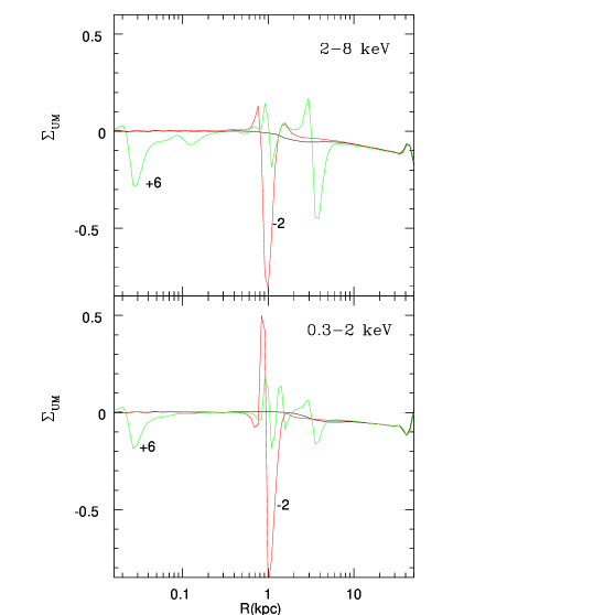
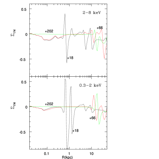
Figure 11: Unsharp masked residuals (Eq. 9) for the gas emission of model B2${}_{02}\,$during outburst, at the same times as in Fig. 8. Note the “cavity” as a decrement in brightness close to the center, at $+6$, $+18$ and $+66$ Myr, and the surrounding bright and sharp rim; both features are similar to what revealed by unsharp masking in a few well studied ellipticals (e.g., NGC4552, Machacek et al. 2006).

The behavior of the gas during an outburst is almost independent of the specific burst episode considered. The outburst precursor is the off-center growth of a thin shell of dense gas (at a radius of $\sim 0.5-1$ kpc) that progressively cools below X-ray emitting temperatures and falls towards the center; compression of the enclosed gas follows and a central burst is triggered, even before the cold shell reaches the center. In less than a million years, a radiative shock originates from the center and quickly (in $\approx 10^{6}$ yrs) produces an outward moving shell that collides with the original shell falling in. Reflected shock waves carry fresh material for accretion, and produce new sub-bursts. This leads to the rich temporal structure of each outburst event, especially visible in model B3${}_{02}\,$(bottom panel, Fig. 1). Eventually, the cold material left after starformation (Ciotti & Ostriker 2007) is accreted in a final burst, a major shock leaves behind a very hot and dense center, and causes a substantial galaxy degassing. In general, while radiative effects mainly work on the kpc scale, mechanical feedback from the AGN winds is more concentrated and affects the ISM on the $\sim 100$ pc scale (see Fig. 11 in Paper III). During the next few tens of million years, the gas cools, resumes its subsonic velocity, the density starts increasing again due to stellar mass losses, and the cycle repeats. At late epochs, the gas flows finally set in a state of steady, hot and low-luminosity accretion.

3 Observational properties of the models

The observational model properties considered in Paper III were the nuclear bolometric, optical and UV luminosities, and the X-ray luminosity of the ISM within $10R_{\rm e}$. The latter was evaluated fiducially just by cutting the bolometric gas emission below a threshold temperature of $5\times 10^{6}$ K. In the following, we calculate the X-ray luminosity of the nucleus ($L_{\rm BH,X}$, Sect. 4), and, with a more detailed and realistic procedure, the total luminosity and emission weighted temperature of the hot gas ($L_{\rm X}$ and $<T_{\rm X}>$, Sect. 5); we also calculate the temperature and the surface brightness profiles during quiescent times, and during an outburst (Sect. 6). We briefly describe below how the observational gas properties are calculated from the numerical outputs for the gas density and temperature.

The X-ray emission of the different model components is calculated over the energy range of 0.3-8 keV (the $Chandra$ sensitivity band), and also in two separate bands, 0.3-2 keV (“soft”) and 2-8 keV (“hard”), typically used in studies of the nuclear and gaseous properties. In practice, at any given time, the volume gas luminosity is calculated from the gas density and temperature distribution on the numerical grid as

$$L_{\rm X}=4\pi\int_{0}^{\infty}{\cal{E}}(r)r^{2}dr,$$ (2)

where the emissivity is given by ${\cal{E}}(r)=n_{\rm e}(r)n_{\rm H}(r)\Lambda[T(r),Z]$, $n_{\rm e}$ and $n_{\rm H}$ are the number densities of electrons and hydrogen, and $\Lambda(T,Z)$ is the cooling function. The cooling function is calculated over the two energy intervals by means of the radiative emission code APEC, valid for hot plasmas at the collisional ionization equilibrium (Smith et al. 2001), as available in the XSPEC package for the analysis of the X-ray data. For simplicity we choose constant abundance at the solar value, and the solar abundance ratios of Grevesse & Sauval (1998), which is consistent with observed gas metallicities (e.g., Loewenstein & Davis 2010). In order to speed-up the analysis, we derived with APEC the values of $\Lambda$, for each energy band, for a large set of temperatures in the range 0.1-16 keV; then we obtained two very accurate non-linear fits of the tabulated values (with maximum deviations $<1$%, see Ciotti & Pellegrini 2008). These fits were used to compute the integral in (2), and in every other integration where the emissivity is needed. For example the emission weighted temperature for the whole galactic volume was computed as

$$<T_{\rm X}>={4\pi\over L_{\rm X}}\int_{0}^{\infty}{\cal{E}}(r)T(r)r^{2}dr.$$ (3)

The surface brightness profile $\Sigma(R)$, the emission weighted projected temperature profile $T_{\rm p}(R)$, and the associated emission weighted aperture temperature profile $T_{\rm a}(R)$, were obtained by numerical integration of the simulation outputs as

$$\Sigma(R)=2\int_{R}^{\infty}{{\cal{E}}(r)r\over\sqrt{r^{2}-R^{2}}}dr,$$ (4)

$$T_{\rm p}(R)={2\over\Sigma(R)}\int_{R}^{\infty}{T(r){\cal{E}}(r)r\over\sqrt{r^{2}-R^{2}}}dr,$$ (5)

$$T_{\rm a}(R)={\int_{0}^{R}T_{\rm p}(R^{\prime})\Sigma(R^{\prime})R^{\prime}dR^{\prime}\over\int_{0}^{R}\Sigma(R^{\prime})R^{\prime}dR^{\prime}}.$$ (6)

The accuracy of the integrations above is verified by checking that the surface integral of $\Sigma(R)$ over the whole grid recovers the same luminosity calculated via equation (2), and that $T_{\rm a}(\infty)=<T_{\rm X}>$ within few percent (Ciotti & Pellegrini 2008). The surface integral of $\Sigma(R)$ is also used to compute the gas emission within the optical effective radius $R_{\rm e}$, and in equation (6) to compute the average temperature within the optical effective radius.

In order to highlight local departures from the mean ISM brightness profile, and to evidence major brightness features that could be revealed by observations, “fluctuation” profiles have been also created. These have been constructed with a technique similar to the so-called unsharp masking, frequently adopted in observational analysis (e.g., Fabian et al. 2003). In practice, the brightness profiles $\Sigma(R)$ have been convolved with a 2D Gaussian of dispersion $\sigma$:

$${\rm PSF}={e^{-{R^{2}\over 2\sigma^{2}}}\over 2\pi\sigma^{2}},$$ (7)

so that the resulting surface brightness profile can be written as

$$\Sigma_{\rm obs}(R)=\int_{0}^{\infty}{\rm I}_{0}\left({RR^{\prime}\over\sigma^{2}}\right)\,\,{e^{-{R^{\prime 2}+R^{2}\over 2\sigma^{2}}}\over\sigma^{2}}\,\,\Sigma(R^{\prime})R^{\prime}dR^{\prime},$$ (8)

where I₀ is the zeroth-order modified Bessel function of first kind. In the analysis of the simulations, the integral above is solved numerically, after a careful choice of $\sigma$. As expected, a too large $\sigma$ produces an almost featureless profile, while a too small $\sigma$ reproduces the unprocessed profile. After some attempts, it turned out that, in order to highlight local features, the optimal choice is that of a $\sigma$ equal, at each gridpoint, to the sum of the lengths of the immediately preceding and subsequent grid intervals. The “unsharp-masked” profile is then defined in a natural way as

$$\Sigma_{\rm UM}(R)\equiv{\Sigma(R)\over\Sigma_{\rm obs}(R)}-1.$$ (9)

4 Nuclear luminosities

Figure 1 shows the time evolution of the nuclear bolometric accretion luminosity $L_{\rm BH}$ for B2${}_{02}\,$and B3${}_{02}\,$(whose input parameters differ only for the maximum value of the mechanical efficiency $\epsilon_{\rm w}^{\rm M}$, that is respectively $10^{-3}$ and $3\times 10^{-4}$, Tab. 1). Strong intermittencies at an earlier epoch, with $L_{\rm BH}$ reaching the Eddington value, become rarer and rarer with time, as the mass return rate from the stellar population declines, until a smooth, hot, and very sub-Eddington accretion phase establishes. The different mechanical efficiency is responsible for the sharp bursts in model B2${}_{02}\,$, and the more time-extended and structured bursts in model B3${}_{02}\,$(Paper III). Towards the present epoch, at a galaxy age of 12 Gyr, the mass accretion rate on the MBH for both models is $\dot{M}_{\rm BH}\approx 0.02\,M_{\odot}$/yr, that translates into an Eddington scaled accretion rate $\dot{m}\simeq 1.7\times 10^{-3}$ and $\dot{m}\simeq 1.2\times 10^{-3}$ respectively for B2${}_{02}\,$and B3${}_{02}\,$. The value of $\dot{m}$ of B3${}_{02}\,$is a bit smaller than for B2${}_{02}\,$, because of its larger final $M_{\rm BH}$ (Tab. 2), a consequence of the weaker mechanical feedback. At the present time, and during the interburst periods, accretion has then entered the RIAF regime, and the radiative efficiency is $\epsilon\simeq 0.02$; the nuclear bolometric luminosity is $L_{\rm BH}=2.4\times 10^{43}$ erg s^-1 for both models, and the corresponding Eddington ratios are $l\simeq 2\times 10^{-4}$ (B2${}_{02}\,$) and $l\simeq 10^{-4}$ (B3${}_{02}\,$), see Tab. 2.

These results agree with the observation that in the local universe massive MBHs are mostly radiatively quiescent, and the fraction of them at luminosities approaching their Eddington limit is negligible (e.g., Ho 2008). For example, in the sample of nuclei of the Palomar Spectroscopic Survey of northern galaxies, a nearly complete sample, magnitude limited at $B_{\rm T}\leq 12.5$ mag, $\sim 50$% of ellipticals show detectable emission line nuclei, but mostly of low level ($L_{\rm H\alpha}<10^{40}$ erg/s; Ho 2008). For this sample, the nuclear bolometric luminosity $(L_{\rm bol,nuc})$ was derived from the observed nuclear 2-10 keV emission, using the correction $L_{\rm bol,nuc}/L_{\rm X,nuc}=15.8$ (Ho 2009). It was found that elliptical galaxies span a large range of $L_{\rm bol,nuc}$, from $10^{38}$ to $10^{43}$ erg s^-1, with a median value of $L_{\rm bol,nuc}\simeq 1.7\times 10^{40}$ erg s^-1 and a mean value of $4.6\times 10^{41}$ erg s^-1; the Eddington scaled luminosity $l$ has a median value of $l=1.2\times 10^{-6}$ (mean $l=1.2\times 10^{-5}$), with $l<10^{-3}$ for elliptical galaxies, and extending down to $l=10^{-8}$. The representative models tend therefore to lie on the upper end of the observed distributions of $L_{\rm bol,nuc}$ and $l$, a result that probably remains true regardless of the uncertainty in the bolometric correction from the 2-10 keV band. We will return on this point (already noticed in Papers I and III) in the Conclusions.

Another way of comparing the model $L_{\rm BH}$ with observed values, is to estimate $L_{\rm BH,X}$ of the models, and compare it directly with observed $L_{\rm X,nuc}$ values. Accurate $L_{\rm X,nuc}$ measurements in a large number have been derived recently for elliptical galaxies of the local universe, based on $Chandra$ data (e.g., Gallo et al. 2010, Pellegrini 2010); in the 0.3–10 keV band, $L_{\rm X,nuc}$ ranges from ${\mathrel{\mathchoice{\lower 2.9pt\vbox{\halign{$\m@th\displaystyle\hfil#\hfil$\cr>\crcr\sim\crcr}}}{\lower 2.9pt\vbox{\halign{$\m@th\textstyle\hfil#\hfil$\cr>\crcr\sim\crcr}}}{\lower 2.9pt\vbox{\halign{$\m@th\scriptstyle\hfil#\hfil$\cr>\crcr\sim\crcr}}}{\lower 2.9pt\vbox{\halign{$\m@th\scriptscriptstyle\hfil#\hfil$\cr>\crcr\sim\crcr}}}}}10^{38}$ erg s^-1 to $\sim 10^{42}$ erg s^-1, with most of $L_{\rm X,nuc}/L_{\rm Edd}$ as low as $10^{-6}$–$10^{-8}$. In particular, for the final MBH masses of the models (Tab. 2), it is observed that $10^{38}{\mathrel{\mathchoice{\lower 2.9pt\vbox{\halign{$\m@th\displaystyle\hfil#\hfil$\cr<\crcr\sim\crcr}}}{\lower 2.9pt\vbox{\halign{$\m@th\textstyle\hfil#\hfil$\cr<\crcr\sim\crcr}}}{\lower 2.9pt\vbox{\halign{$\m@th\scriptstyle\hfil#\hfil$\cr<\crcr\sim\crcr}}}{\lower 2.9pt\vbox{\halign{$\m@th\scriptscriptstyle\hfil#\hfil$\cr<\crcr\sim\crcr}}}}}L_{\rm X,nuc}$(erg s${}^{-1}){\mathrel{\mathchoice{\lower 2.9pt\vbox{\halign{$\m@th\displaystyle\hfil#\hfil$\cr<\crcr\sim\crcr}}}{\lower 2.9pt\vbox{\halign{$\m@th\textstyle\hfil#\hfil$\cr<\crcr\sim\crcr}}}{\lower 2.9pt\vbox{\halign{$\m@th\scriptstyle\hfil#\hfil$\cr<\crcr\sim\crcr}}}{\lower 2.9pt\vbox{\halign{$\m@th\scriptscriptstyle\hfil#\hfil$\cr<\crcr\sim\crcr}}}}}10^{42}$, and $10^{-9}{\mathrel{\mathchoice{\lower 2.9pt\vbox{\halign{$\m@th\displaystyle\hfil#\hfil$\cr<\crcr\sim\crcr}}}{\lower 2.9pt\vbox{\halign{$\m@th\textstyle\hfil#\hfil$\cr<\crcr\sim\crcr}}}{\lower 2.9pt\vbox{\halign{$\m@th\scriptstyle\hfil#\hfil$\cr<\crcr\sim\crcr}}}{\lower 2.9pt\vbox{\halign{$\m@th\scriptscriptstyle\hfil#\hfil$\cr<\crcr\sim\crcr}}}}}L_{\rm X,nuc}/L_{\rm Edd}{\mathrel{\mathchoice{\lower 2.9pt\vbox{\halign{$\m@th\displaystyle\hfil#\hfil$\cr<\crcr\sim\crcr}}}{\lower 2.9pt\vbox{\halign{$\m@th\textstyle\hfil#\hfil$\cr<\crcr\sim\crcr}}}{\lower 2.9pt\vbox{\halign{$\m@th\scriptstyle\hfil#\hfil$\cr<\crcr\sim\crcr}}}{\lower 2.9pt\vbox{\halign{$\m@th\scriptscriptstyle\hfil#\hfil$\cr<\crcr\sim\crcr}}}}}10^{-4}$, both from the sample of the $Hubble$ Virgo Cluster Survey (Gallo et al. 2010), and that of 112 early type galaxies within $\sim 60$ Mpc (Pellegrini 2010). The 0.3-10 keV nuclear luminosity $L_{\rm BH,X}$ of the models at the present epoch can be derived adopting a correction factor appropriate for the spectral energy distribution of a radiatively inefficient accretion flow, i.e., $L_{\rm BH,X}{\mathrel{\mathchoice{\lower 2.9pt\vbox{\halign{$\m@th\displaystyle\hfil#\hfil$\cr<\crcr\sim\crcr}}}{\lower 2.9pt\vbox{\halign{$\m@th\textstyle\hfil#\hfil$\cr<\crcr\sim\crcr}}}{\lower 2.9pt\vbox{\halign{$\m@th\scriptstyle\hfil#\hfil$\cr<\crcr\sim\crcr}}}{\lower 2.9pt\vbox{\halign{$\m@th\scriptscriptstyle\hfil#\hfil$\cr<\crcr\sim\crcr}}}}}0.2L_{\rm BH}$ for low luminosity AGNs (Mahadevan 1997). This gives $L_{\rm BH,X}{\mathrel{\mathchoice{\lower 2.9pt\vbox{\halign{$\m@th\displaystyle\hfil#\hfil$\cr<\crcr\sim\crcr}}}{\lower 2.9pt\vbox{\halign{$\m@th\textstyle\hfil#\hfil$\cr<\crcr\sim\crcr}}}{\lower 2.9pt\vbox{\halign{$\m@th\scriptstyle\hfil#\hfil$\cr<\crcr\sim\crcr}}}{\lower 2.9pt\vbox{\halign{$\m@th\scriptscriptstyle\hfil#\hfil$\cr<\crcr\sim\crcr}}}}}5\times 10^{42}$ erg s^-1, and $L_{\rm BH,X}/L_{\rm Edd}{\mathrel{\mathchoice{\lower 2.9pt\vbox{\halign{$\m@th\displaystyle\hfil#\hfil$\cr<\crcr\sim\crcr}}}{\lower 2.9pt\vbox{\halign{$\m@th\textstyle\hfil#\hfil$\cr<\crcr\sim\crcr}}}{\lower 2.9pt\vbox{\halign{$\m@th\scriptstyle\hfil#\hfil$\cr<\crcr\sim\crcr}}}{\lower 2.9pt\vbox{\halign{$\m@th\scriptscriptstyle\hfil#\hfil$\cr<\crcr\sim\crcr}}}}}2\times 10^{-5}$. Also in the X-ray band, then, the model nuclear luminosity tends to be larger than what typically observed; $L_{\rm BH,X}/L_{\rm Edd}$ is within the observed range, though lying in its upper end. All this may suggest that in real galaxies an additional mechanism is reducing further the mass available for accretion, as could be provided by a nuclear jet, and/or a thermally driven wind from a RIAF (Blandford & Begelman 1999). In the latter case, only a fraction of the gas within the accretion radius actually reaches the MBH; the binding energy released by the accreting gas is transported radially outward to drive away the remainder in the form of a wind.

Alternatively, it may be that the quadratic dependence of $l$ on $\dot{m}$ (Sect. 2) sets in at a higher value of $\dot{m}$ than adopted in Eq. 1, for which it starts at $\dot{m}\sim 10^{-2}$. Within the uncertainties on the observational and theoretical input, we might have chosen the constant $A=10$ rather than 100; in this way, the quadratic dependence would have set in at $l{\mathrel{\mathchoice{\lower 2.9pt\vbox{\halign{$\m@th\displaystyle\hfil#\hfil$\cr<\crcr\sim\crcr}}}{\lower 2.9pt\vbox{\halign{$\m@th\textstyle\hfil#\hfil$\cr<\crcr\sim\crcr}}}{\lower 2.9pt\vbox{\halign{$\m@th\scriptstyle\hfil#\hfil$\cr<\crcr\sim\crcr}}}{\lower 2.9pt\vbox{\halign{$\m@th\scriptscriptstyle\hfil#\hfil$\cr<\crcr\sim\crcr}}}}}0.1$ rather than $l{\mathrel{\mathchoice{\lower 2.9pt\vbox{\halign{$\m@th\displaystyle\hfil#\hfil$\cr<\crcr\sim\crcr}}}{\lower 2.9pt\vbox{\halign{$\m@th\textstyle\hfil#\hfil$\cr<\crcr\sim\crcr}}}{\lower 2.9pt\vbox{\halign{$\m@th\scriptstyle\hfil#\hfil$\cr<\crcr\sim\crcr}}}{\lower 2.9pt\vbox{\halign{$\m@th\scriptscriptstyle\hfil#\hfil$\cr<\crcr\sim\crcr}}}}}0.01$. This would have reduced the late time nuclear luminosity by a factor of $\simeq 9$, as confirmed by a supplementary run of models B2${}_{02}\,$and B3${}_{02}\,$with $A=10$.

Finally, another interesting - albeit more difficult - comparison with observational results can be done using the duty-cycle. The latter can be calculated as the fraction of the total time spent by the AGN in the “on” state, defined by a luminosity greater than $L_{\rm Edd}/30$ in a given band, over some temporal baseline (Paper III). So doing, the duty-cycle turns out to be a small number (Tab. 2); for example, for a temporal baseline ending at the present epoch (i.e., at 13 Gyr in Fig. 1), the duty-cycle of model B2${}_{02}\,$is zero when starting from 9 Gyr (at a redshift $z\approx 0.45$, for a flat universe with $H_{0}=71$ km s^-1 Mpc^-1, $\Omega_{M}=0.27$, $\Omega_{\Lambda}=0.73$), as no burst occurs after $\simeq 7.5$ Gyr; when starting from 6 Gyr ($z\approx 1$), it is $\simeq 6.3\times 10^{-3}$, $3.2\times 10^{-3}$, and $3.0\times 10^{-3}$ respectively in the bolometric, optical (absorbed), and UV (absorbed) bands. For model B3${}_{02}\,$, in the same bands, the duty-cycle is respectively $\simeq 4.9\times 10^{-2},1.7\times 10^{-2},7.1\times 10^{-3}$ (when starting at 9 Gyr), and $\simeq 4.8\times 10^{-2},1.8\times 10^{-2},8.6\times 10^{-3}$ (when starting at 6 Gyr). The duty-cycle decreases from the bolometric, to the optical, to the UV bands, due to the different values of the opacity in these bands.

These duty-cycle values are broadly consistent with the fraction of active galaxies measured in observational works. For example, Greene & Ho (2007) estimated the (mass dependent) number of active galaxies, using broad-line luminosities from SDSS DR4, for galaxies with $z<0.352$ (age of the universe ${\mathrel{\mathchoice{\lower 2.9pt\vbox{\halign{$\m@th\displaystyle\hfil#\hfil$\cr>\crcr\sim\crcr}}}{\lower 2.9pt\vbox{\halign{$\m@th\textstyle\hfil#\hfil$\cr>\crcr\sim\crcr}}}{\lower 2.9pt\vbox{\halign{$\m@th\scriptstyle\hfil#\hfil$\cr>\crcr\sim\crcr}}}{\lower 2.9pt\vbox{\halign{$\m@th\scriptscriptstyle\hfil#\hfil$\cr>\crcr\sim\crcr}}}}}10$ Gyr); statistically speaking, the fraction of active systems can be interpreted as a duty cycle for MBHs in a given mass range. Greene & Ho report duty-cycle values of the order of $4\times 10^{-3}$ for $10^{7}$ $M_{\odot}$ MBHs, declining at increasing mass. Similar duty-cycle values of $\sim 2\times 10^{-3}$, decreasing at increasing MBH mass, are reported by Heckman et al. (2004). The duty-cyles of the models tend to be larger than those observed; however, the comparison is limited by the small number of models considered, and the fact that the only way to compute duty-cycles different from zero is to extend the temporal baseline back in the past. A more consistent comparison with observations can be made with an increased dataset of models, and computing the duty cycle for the last 2–3 Gyrs. Clearly this procedure will reduce the duty cycle, as the models are characterized by a declining nuclear activity. Again, the computed duty cycle would have been reduced significantly also if we had raised the threshold for RIAF-like behavior of the radiative efficiency to $l=0.1$.

5 Luminosity and Temperature of the Gas

We describe here the time evolution of the global thermal luminosity and temperature of the ISM.

5.1 Luminosity evolution

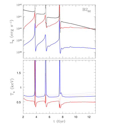
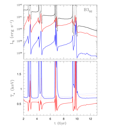
Figure 2: Time evolution, shown with solid lines, of the ISM X-ray luminosity $L_{\rm X}$ (upper panels) and emission-weighted temperature $T_{\rm a}$ (lower panels), both calculated within an aperture of $10R_{\rm e}$, for model B2${}_{02}\,$(left panels) and B3${}_{02}\,$(right panels). Red and blue lines refer to the 0.3-2 keV and 2-8 keV bands. For reference, the black dotted line in the upper panels shows $L_{\rm BH}$ scaled down by a factor of 2000 from Fig. 1. In the bottom panels, the dotted lines show $T_{\rm a}(R_{\rm e})$; in each band, $T_{\rm a}(R_{\rm e})$ is higher than $T_{\rm a}(10R_{\rm e})$. Note the characteristic opposite trend of the red and blue temperatures during the bursts, a clear sign of the coexistence of hot (central bubble) and cold (radiative shells) ISM phases. Temperatures computed over the whole 0.3–8 keV energy interval (not shown here) are always very close to those weighted with the 0.3–2 keV emission, except during the burst times. See Sect. 5 for more details.

The top panels of Fig. 2 show the time evolution of the total gas emission $L_{\rm X}$ for models B2${}_{02}\,$(left) and B3${}_{02}\,$(right). Red lines refer to the soft (0.3-2 keV) band, and blue lines to the hard (2-8 keV) band; for reference, the scaled-down $L_{\rm BH}$ (black dotted line) is also shown.

The luminosity evolution of the gas for the two models is qualitatively similar, with peaks in $L_{\rm X}$ coinciding with those in $L_{\rm BH}$. The sudden increase of the gas emission during outbursts is due to the increase in temperature and density in the central galactic regions ($\simeq 10^{2}-10^{3}$ pc), caused by radiative gas heating (Compton and photoionization), and by compression due to direct and reflected shock waves, produced by mechanical and radiative feedback, that are associated with the AGN and the starburst. For short times, most of the luminosity in the peaks of $L_{\rm X}$ originates from a very small region at the galactic center ($\approx 100$ pc), thus it is observationally indistinguishable from the luminosity of the nucleus (see also Sect. 6.2). The hard emission oscillates in phase with the soft one, and presents the same overall behavior, but keeps at a level almost 2 orders of magnitude lower. Hard emission during the outburst, as shown in Fig. 2, would be detectable with $Chandra$, if centrally concentrated (see also Sect. 6.2 below). However, hard emission during quiescent times would be difficult to distinguish from the contribution of unresolved binaries, even with $Chandra$, if extended (e.g., Pellegrini et al. 2007, Trinchieri et al. 2008).

A comparison of the peaks in $L_{\rm X}$ and $L_{\rm BH}$ reveals differences and analogies. While $L_{\rm BH}$ shows sharp and sudden spikes at the outbursts (increasing by 2 or more orders of magnitude in $\approx 10^{6-7}$ yr), and is almost constant between them, $L_{\rm X}$ increases slowly but steadily between outbursts, when the galaxy is replenished by the stellar mass losses. The peaks in $L_{\rm X}$ become broader with increasing time, but not weaker; for example, the increase of $L_{\rm X}$ during the last major outburst of B2${}_{02}\,$is the largest one, with the largest amount of gas heated and then removed from the galaxy in its entire life. Instead, when the burst ends, $L_{\rm X}$ has the same abrupt decrease as $L_{\rm BH}$, due to the density drop following the final (and usually strongest) sub-burst in each major accretion event. Another similarity is that both $L_{\rm BH}$ and $L_{\rm X}$ show sharper and “cleaner” bursts in B2${}_{02}\,$than in B3${}_{02}\,$: more radiatively dominated feedback bursts (as in B3${}_{02}\,$) are richer in temporal substructure, because it takes longer for the cold shells to be destroyed, thus more star formation and MBH accretion occurs (Paper III).

The quiescent values of $L_{\rm X}$ during the past few Gyr remain at the same level of $\sim 10^{40}$ erg s^-1 for model B2${}_{02}\,$, and decrease by a small factor of ${\mathrel{\mathchoice{\lower 2.9pt\vbox{\halign{$\m@th\displaystyle\hfil#\hfil$\cr<\crcr\sim\crcr}}}{\lower 2.9pt\vbox{\halign{$\m@th\textstyle\hfil#\hfil$\cr<\crcr\sim\crcr}}}{\lower 2.9pt\vbox{\halign{$\m@th\scriptstyle\hfil#\hfil$\cr<\crcr\sim\crcr}}}{\lower 2.9pt\vbox{\halign{$\m@th\scriptscriptstyle\hfil#\hfil$\cr<\crcr\sim\crcr}}}}}2$ to reach a present epoch $L_{\rm X}=2\times 10^{39}$ erg s^-1 for B3${}_{02}\,$. Previous compilations of observed $L_{\rm X}$ values (Fabbiano et al. 1992, O’Sullivan et al. 2001, Diehl & Statler 2007, Mulchaey & Jeltema 2010) for early type galaxies of the local universe, residing in all kinds of environments (from the field to groups to clusters as Virgo and Fornax), show a range of $L_{\rm X}$ from $10^{40}$ erg s^-1 up to $10^{43}$ erg s^-1, at a B-band optical luminosity of $L_{\rm B}=5\times 10^{10}L_{\rm B,\odot}$ as the model galaxy. $L_{\rm X}$ values larger than a few$\times 10^{41}$ erg s^-1 belong to galaxies at the center of groups, or clusters, or subclusters, for which an important contribution from the intragroup or intracluster medium, or a confining action, is likely (e.g., Renzini et al. 1993, Brighenti & Mathews 1998, Brown & Bregman 2000, Helsdon et al. 2001). However, the final $L_{\rm X}$ of B2${}_{02}\,$and B3${}_{02}\,$is on the lower end of the range of observed values; this indicates that degassing is important in the models, and for many real cases it must be impeded. In the simulations this could be obtained for example by adding the external pressure from an outer medium (e.g., Vedder et al. 1988), and it will be considered in future works.

5.1.1 $L_{\rm X}-L_{\rm B}$ and $L_{\rm X}-L_{\rm BH}$

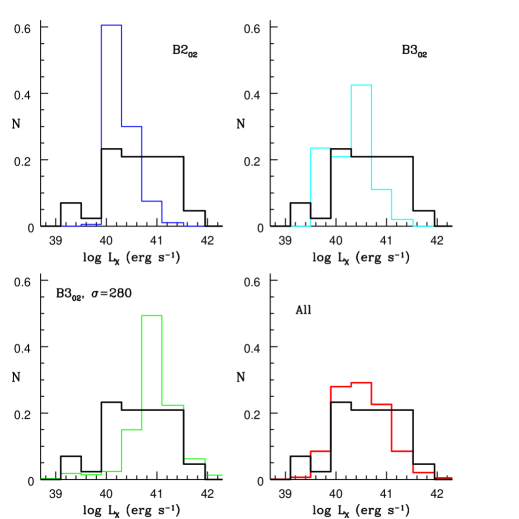
Figure 3: Normalized histograms of the 0.3–2 keV gas emission within $10R_{\rm e}$ during the epoch from 2 to 12 Gyrs (colored lines), for the models indicated in each panel, and for their average (bottom right); the variant of B3${}_{02}\,$with $\sigma$ increased to 280 km s^-1 (bottom left panel) is taken from Ciotti & Ostriker 2011. The histograms are compared with the histogram of observed luminosity values (converted to the 0.3–2 keV band), for non-AGN and non-central cluster or group members, with log$L_{B}$ in the range from 10.5 to 10.8 (black line; values from the $ROSAT$ sample of local early type galaxies, O’Sullivan et al. 2001; their estimate of the stellar source contribution has been subtracted to the observed $L_{X}$).

Real galaxies show a wide range of $L_{\rm X}$ values, and the observed $L_{\rm X}$ variation has remained a subject of debate for years (e.g., Fabbiano et al. 1989, Ciotti et al. 1991, White & Sarazin 1991; Pellegrini 2011). Thus, we check here whether the $L_{\rm X}$ variation in the models during their evolution can (partly) account for the large observed one. For this check we considered the range of hot gas emission for the largest sample of early type galaxies of the local universe (O’Sullivan et al. 2001), after having excluded AGN-dominated cases, and central dominant cluster or group galaxies. Only galaxies with optical luminosites within a range close to that of the model galaxy have been considered (i.e., from log$L_{B}=10.5$ to log$L_{B}=10.8$, for which there are 43 galaxies). The discrete stellar sources contribution estimated by O’Sullivan et al. (2001) has been removed. The distribution of the observed X-ray emission values so obtained is then compared with that built for the soft X-ray emission of the models, during the epoch from 2 to 12 Gyrs (Fig. 3). Each emission value enters the histogram with the fraction of the chosen epoch during which it is present; the hypothesis underlying this comparison is that statistically an observed galaxy can be catched in anyone of the different phases shown in the past 2–12 Gyr by the representative models.

Figure 3 shows that $L_{\rm X}$ of the models keeps within the observed range, but it does not exceed significantly $\sim 10^{41}$ erg s^-1, while a fraction of galaxies populates this region. Model B2${}_{02}\,$has a $\sim$constant $L_{X}$ in the past few Gyrs, so that it populates mostly a couple of bins; model B3${}_{02}\,$(that experiences more outbursts) reaches a wider coverage of the observed $L_{X}$ range, but its $L_{X}$ distribution extends more to lower $L_{X}$ values than to larger ones, due to a larger overall degassing. Larger $L_{\rm X}$ for the models can be obtained when considering that real galaxies of similar $L_{\rm B}$ can have different values of the central stellar velocity dispersion and effective radius. These differences determine a variety of flow evolution, and then of $L_{\rm X}$ (Ciotti & Ostriker 2011). Following this idea, Fig. 3 (bottom left) shows the histogram of one possible variation to model B3${}_{02}\,$, that with $\sigma=280$ km s^-1; this indeed reaches larger $L_{\rm X}$ values. Finally, the bottom right panel shows the average of the histograms of the three models, and shows how this average reproduces the observed histogram reasonably well. Overall, this analysis shows that the large observed variation in $L_{\rm X}$ at similar optical $L_{\rm B}$ has another contributing factor, that is nuclear activity, in addition to those already put forward.

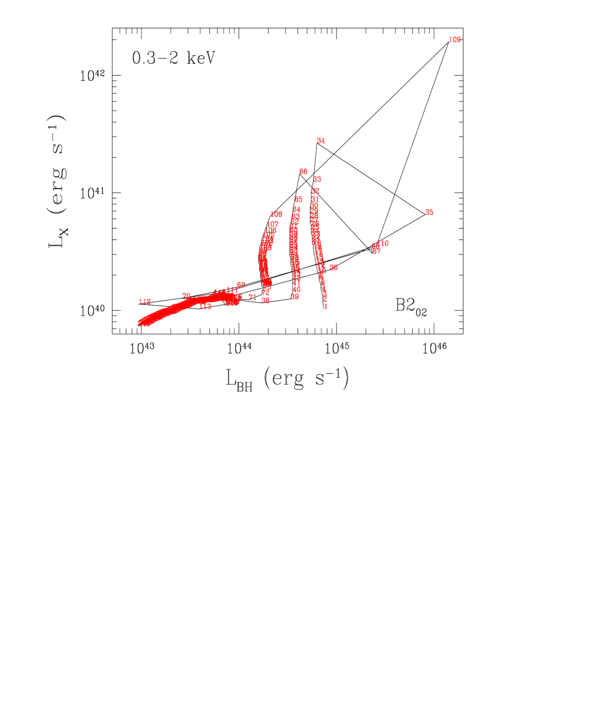
Figure 4: The total 0.3-2 keV gas emission versus the bolometric nuclear radiative output $L_{\rm BH}$, for model B2${}_{02}\,$. The time evolution from 2 to 14 Gyrs corresponds to the increasing numbers along the curve; the time sampling is uniform, i.e., every two subsequent points are 50 Myr distant in time.

Another useful diagram for an observational comparison is given by the relationship between $L_{\rm BH}$ and $L_{\rm X}$; this is shown in Fig. 4, considering all the available temporal outputs, for model B2${}_{02}\,$. The analogous figure for model B3${}_{02}\,$is very similar, with the only difference being the broader temporal extension of the bursts. One can recognize the interburst times, when the galaxy is replenished by stellar mass losses, as periods with $L_{\rm BH}$ almost constant, and $L_{\rm X}$ increasing (which produces almost vertical lines). During outbursts, the soft $L_{\rm X}$ and $L_{\rm BH}$ abruptly increase and then decrease, which produces loops running clockwise on the right of each vertical line; these loops are occupied for a very short time. As time proceeds, the vertical lines (the interburst periods) shift towards lower $L_{\rm BH}$. The final quiescent period is described by a line (the most crowded with numbers) where $L_{\rm BH}$ and $L_{\rm X}$ both decrease, though $L_{\rm BH}$ decreases faster than $L_{\rm X}$. The more the outbursts are confined at earlier epochs, the more the final weak correlation between $L_{\rm X}$ and $L_{\rm BH}$ extends with time; instead, the more the outbursts extend towards the present epoch, the more a trend is expected for $L_{\rm X}$ to increase with $L_{\rm BH}$ with a large scatter around it (as produced by the vertical lines, where galaxies reside most of the time, and by the loops). For a sample of early type galaxies of the local universe, the relationship between $L_{\rm X}$ and the nuclear emission $L_{\rm X,nuc}$ indeed shows a weak trend, dominated by a large scatter (Pellegrini 2010); in the present framework, such an observation could be explained with many galaxies being still in the phases made of the vertical rise followed by the loop. The comparison cannot be pushed farther, though, since the $L_{\rm BH}$ values – when converted to an X-ray band – are typically larger than the observed $L_{\rm X,nuc}$ (Sect. 4).

5.2 Temperature evolution and $L_{\rm X}-T_{\rm a}$

Another important global property of the ISM typically observed is the emission weighted aperture temperature $T_{\rm a}$ (eq. 6), here calculated within the optical $R_{\rm e}$, and within $10R_{\rm e}$. The time evolution of these temperature diagnostics is shown in the bottom panels of Fig. 2, in parallel with the luminosity evolution; red and blue lines again refer to the 0.3–2 keV and 2–8 keV bands, respectively. Note that $T_{\rm a}(10R_{\rm e})$ in the two bands is indistinguishable from the corresponding global emission weighted temperature $<T_{\rm X}>$ (that is calculated but not shown in Fig. 2), as expected given that the density profile is steeply decreasing outward (Paper III); thus $T_{\rm a}(10R_{\rm e})$ is a good proxy for $<T_{\rm X}>$. Also, temperatures computed for the whole 0.3–8 keV band (not shown) are always very close to those weighted with the 0.3–2 keV emission, except for those short burst times during which there is a very hot gas component. As for $L_{\rm X}$, also for $T_{\rm a}$ the temperature peaks of B3${}_{02}\,$are significantly more structured in time than those of B2${}_{02}\,$.

Three main characteristic features of $T_{\rm a}$, common to this class of models, can be pointed out. The first is the complex behavior of $T_{\rm a}$ during outbursts, with variations going in opposite directions for the two bands. This is due to the coexistence of hot (the central bubble) and cold (the radiative shells) ISM phases during the bursts, as revealed by the temporal evolution of the radial profiles of the gas density and temperature (Paper III). The sharp and high peaks in the hard band (blue) correspond to the onset of very hot regions at the center, while the decrements in the soft band (red) are due to a dense cold shell created immediately before the major burst, and to cold gas accumulated by the passage of radiative shock waves produced by the outburst (see also Sect. 6.1).

A second, observationally relevant feature is that in each band $T_{\rm a}(R_{\rm e})$ is higher than $T_{\rm a}(10R_{\rm e})$, which is especially evident in the interburst periods (Fig. 2). For example, in the quiescent phases, both models show a similar $T_{\rm a}(10R_{\rm e})\simeq 0.4-0.5$ keV in the soft band, while $T_{\rm a}(R_{\rm e})\sim 0.7$ keV. This is explained by the radial temperature distribution decreasing outward (Sect. 6.1).

Finally, for model B2${}_{02}\,$Fig. 5 shows the relationship between $L_{\rm X}$ and $T_{\rm a}(10R_{\rm e})$, both calculated for the 0.3–8 keV band; such a diagram is often produced in observational works, for galaxies of all $\sigma$ (e.g., Pellegrini 2011). During the long interburst epochs, $L_{\rm X}$ increases with little variation of $T_{\rm a}$. In the short burst episodes, $L_{\rm X}$ and $T_{\rm a}$ reach a maximum, and then follow a clockwise loop on the right, reach back the original $T_{\rm a}$ value, move left of it, and follow a counterclockwise smaller loop. Then the cycle repeats with $L_{\rm X}$ increasing and $T_{\rm a}$ almost constant. During the last few Gyr, $L_{\rm X}$ remains at $\sim 10^{40}$ erg s^-1 and $T_{\rm a}\sim 0.5$ keV.

We now compare these results with observations. In the largest sample of global, soft X-ray emission weighted temperatures, derived from $ROSAT$ observations, $<T_{\rm X}>$ is in the range $\sim 0.4-0.8$ keV, for galaxies with $\sigma\simeq 260$ km s^-1, as for the model galaxy (O’Sullivan et al. 2003); $T_{\rm a}(10R_{\rm e})$ of the models during quiescence, in the soft band, is within this range, though on its lower end. However various factors tend to bias-high these observed temperatures, as incomplete subtraction of the hard stellar emission due to binaries, or hard AGN emission; in addition, many of the sample galaxies reside in high density environments, with possible contamination from the hotter group/cluster medium, and a temperature profile that is commonly rising outwards (e.g., Diehl & Statler 2008, Nagino & Matsushita 2009), a behavior opposite to that of the models, that refer to isolated galaxies (Sect. 6.1).

$Chandra$ observations, with large sensitivity and much higher angular resolution ($\sim 1^{\prime\prime}$), allowed for an accurate subtraction of all the AGN and stellar sources contributions from the total emission, giving measurements of the gas temperature of unprecedented accuracy (e.g., Boroson et al. 2011). For example, Boroson et al. derived global, 0.3–8 keV emission weighted temperatures, for a few galaxies with $\sigma\sim 260$ km s^-1, ranging from 0.3 to 0.6 keV; $T_{\rm a}(10R_{\rm e})$ of the models agrees very well with this result, falling in the middle of the observed range. Coming to temperature estimates for more central regions, Athey (2007) derived 0.35–8 keV emission weighted temperatures within $R_{\rm e}$, for 53 galaxies with $Chandra$ observations. For a selection of 20 galaxies with $L_{\rm B}$ similar to that of the model galaxy, from log $L_{\rm B}(L_{B,\odot})=10.5$ to 10.8, the average temperature is $0.61\pm 0.03$ keV (calculated weighting each measurement with its uncertainty). Figure 6 shows a full comparison between the distribution of these temperatures and $T_{\rm a}(R_{\rm e})$, calculated for the 0.3–8 keV band, during the evolution of B2${}_{02}\,$and B3${}_{02}\,$. The model $T_{\rm a}(R_{\rm e})$ tends to be concentrated in the upper half of the observed distribution; this result, if confirmed with a larger set of simulated galaxies, indicates that heating in the central galactic region of the models may be too efficient.

In conclusion, the global temperatures of the models fall in the middle of the range of values recently observed, while the model $T_{\rm a}(R_{\rm e})$ reproduces easily the larger observed values and less easily the lower ones.

6 Projected quantities: temperature and brightness profiles

We consider here the radial profiles of the ISM temperature and surface brightness, as they would be revealed for the models by observations. For simplicity we restrict the discussion to model B2${}_{02}\,$, whose sharp bursts allow for an easier presentation; the results are substantially similar for B3${}_{02}\,$. The profiles are constructed using Eqs. 4–9, both during the quiescent phases, that occupy most of the ISM evolution, and during an outburst. The recurrent burst phases are temporally limited, but represent a central aspect of the models, thus they are devoted special attention. Statistically, the feedback features should be present, and possibly revealed by current X-ray observations, in $\simeq 5-10$% of the isolated galaxies with $L_{\rm B}$ similar to that of the models (Sect. 6.2 below). In the following we present snapshots of the projected profiles during quiescence, at an age of 3, 6.5, 9 and 12 Gyr, and centered on the last outburst at 7.5 Gyr.

6.1 Temperature profiles

The emission weighted projected temperature profiles $T_{\rm p}(R)$ during quiescent interburst times are smooth, with the temperature monotonically decreasing for increasing radius (Fig. 7). From an age of 6 Gyr onwards, the temperature keeps at $\simeq 1$ keV at a radius of $\simeq 100$ pc, and at $\sim 0.4$ keV at a radius of $\simeq 30$ kpc. Figure 7 (right panel) shows the corresponding aperture temperature profiles $T_{\rm a}(R)$ calculated in bins (i.e., in Eq. 6 the numerator and denominator are evaluated over radial bins), chosen to reproduce the typical binning used for $Chandra$ observations of nearby galaxies (Humphrey et al. 2006, Diehl & Statler 2007).

Temperature profiles with negative gradients had already been found for gas inflows in steep galactic potentials without feedback, due to compressional heating (e.g., Pellegrini & Ciotti 1998). As typical of models without a central MBH, in that case the temperature also had a central drop. In the present computations, instead, the combined effects of the gravitational field of the MBH, and of the high injection temperature of the stellar mass losses (a consequence of the stellar velocity dispersion that is enhanced by the presence of the MBH, within its sphere of influence), keep the gas temperature increasing approaching the center, even outside the burst episodes (see also Pellegrini 2011). A temperature profile that keeps smoothly decreasing towards the center for a long time, as expected in classical cooling flows, is never shown by the model runs.

With time increasing, the value of the central temperature does not increase significantly after 6 Gyr, since it is mainly determined by the gravitational effects of the MBH, whose mass remains approximately constant. The external $T_{\rm p}(R)$ values instead steadily increase with time, since they are determined by the SNIa’s heating; the latter has a secular trend that produces a time-increasing specific heating of the mass return rate (i.e., $L_{\rm SNIa}/\dot{M}_{*}\propto t^{0.2}$, where $L_{\rm SNIa}$ is the energy injected per unit time by SNIa’s supernova explosions, and $\dot{M}_{*}$ is the stellar mass loss injected per unit time; e.g., see Pellegrini 2011).

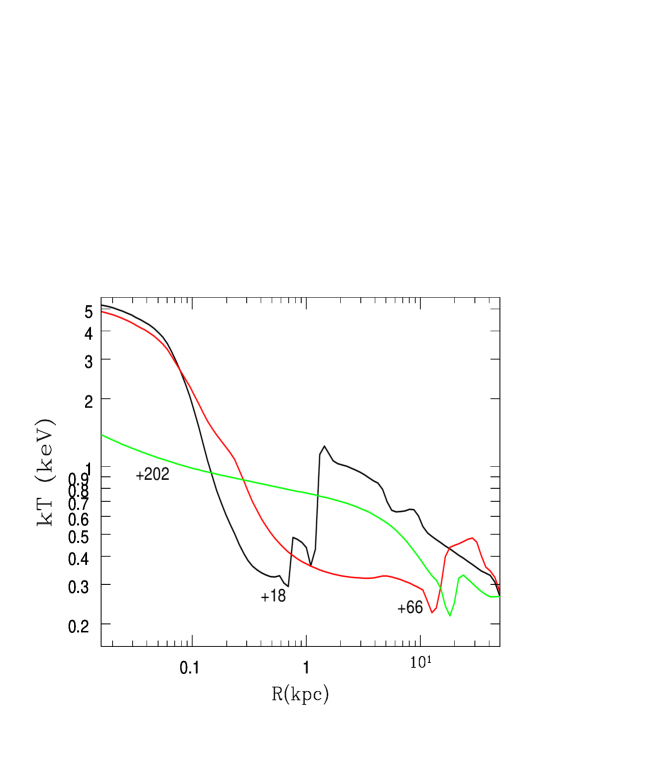
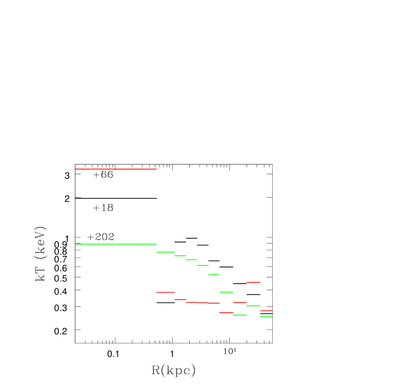
Figure 8: Left panels: radial profiles of the emission-weighted projected temperature $T_{\rm p}(R)$ in the 0.3-8 keV band, during the last major burst of model B2${}_{02}\,$(at $\simeq 7.498$ Gyr). The numbers near the lines indicate the times (in Myr) calculated with respect to the outburst; in the top panel the black line shows the unperturbed profile before the outburst (at a time of 7.400 Gyr). Right panels: the corresponding aperture temperature profiles $T_{\rm a}(R)$, averaged with the surface brightness in bins with the same radial range adopted for Fig. 7.

We now focus on the evolution during the last outburst (Fig. 8). As typical, starting from the unperturbed profile, a shell of denser gas creates, in this case at a radius of $\simeq 800$ pc, particularly evident as a dip in the otherwise monotonically decreasing profile (see the -2 Myr red line in the top left panel). The shell falls towards the center, progressively cooling, so that the soft X-ray emission weighted temperature decreases (Fig. 2, bottom panels). A first AGN burst is produced before the shell reaches the center, and the resulting outward moving shock empties and heats the gas in the inner regions of the galaxy, on a time scale of $\approx 1$ Myr. The subsequent snapshot in Fig. 8, at +6 Myr after the first burst, shows the high central temperature typical of the outburst phase: $T_{\rm p}(R)\sim$few keV within a radius of $\sim 50-100$ pc.

When the shock enters the radiative snow-plow phase, the associated secondary dense shell interacts with the first one still falling, and a series of direct and reflected shock waves are produced, accompanied by accretions events and star formation. The profiles between -2 Myr and +18 Myr (not shown) are very irregular, and consisting of a series of dips propagating outwards, with the temperature in the central region quickly and alternately increasing and decreasing. As already noticed for Fig. 2, both hotter and colder regions are continuously created, the hottest ones within $\sim 1$ kpc (mainly due to shocks), and the coldest ones due to the cooling gas in the shells.

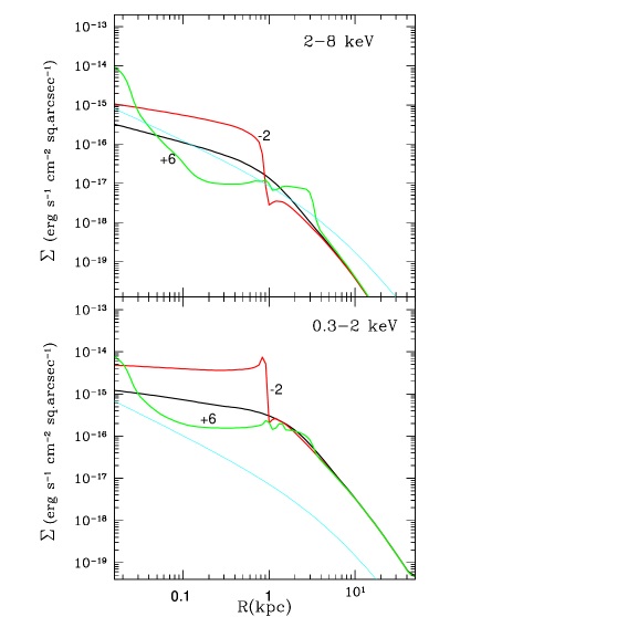
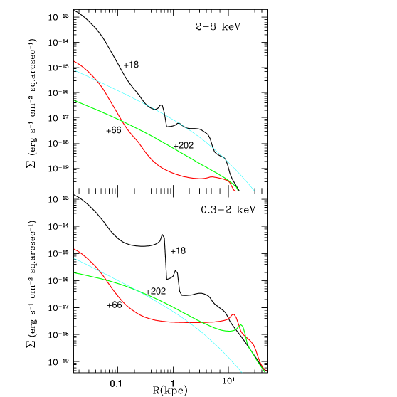
Figure 10: The X-ray brightness profiles in the hard (top panels) and soft (bottom panels) bands, during the last outburst of B2${}_{02}\,$(occurring at 7.498 Gyr), for the same times as in Fig. 8, indicated in Myr close to each curve. The cyan line is an estimate for the unresolved binaries contribution in the two bands, calculated as for Fig. 9. At -2 Myr the outburst is preparing and the shell is developing and approaching the center; after the first outburst the center hosts a hot region (+6 Myr). A hot and dense central region is present also at +18 Myr, while an outward moving shock is still barely visible at +66 Myr and +202 Myr.

Each sub-burst is stronger than the previous one; finally, a last shock from the center concludes the phenomenon, halting star formation and leaving behind a very hot nucleus (the +66 Myr red line), while emptying the rest of the galaxy [see also the $\Sigma(R)$ profile at +66 Myr in Fig. 10]. Then, during the following $\simeq 100$ Myr, the gas resumes the temperature typical of quiescent times (the +202 Myr green line). The inner very hot phase lasts for ${\mathrel{\mathchoice{\lower 2.9pt\vbox{\halign{$\m@th\displaystyle\hfil#\hfil$\cr<\crcr\sim\crcr}}}{\lower 2.9pt\vbox{\halign{$\m@th\textstyle\hfil#\hfil$\cr<\crcr\sim\crcr}}}{\lower 2.9pt\vbox{\halign{$\m@th\scriptstyle\hfil#\hfil$\cr<\crcr\sim\crcr}}}{\lower 2.9pt\vbox{\halign{$\m@th\scriptscriptstyle\hfil#\hfil$\cr<\crcr\sim\crcr}}}}}0.1$ Gyr.

During the bursts, cosmic rays are shock-accelerated, and the inner regions look similar to a gigantic supernova remnant. Only thermal X-rays are considered here, while those due to synchrotron emission from accelerated particles due to shocks were not computed (see Jiang et al. 2010).

The profiles in the right panels of Fig. 8 show the binned aperture temperature profiles, for the same times as for the left panels. The binning smears the small-scale features, but the major distinctive characteristics, as the temperature dip when the first shell forms, and the large temperature drop outside the center, at +18 Myr and +66 Myr, are still well detectable.

6.1.1 Comparison with observed profiles

Negative radial gradients, as shown by the model temperature during quiescence (Fig. 7), are common among ellipticals, as revealed most recently by $Chandra$ observations (e.g., Kim & Fabbiano 2003, Humphrey et al. 2006, Sansom et al. 2006, Fukazawa et al.  2006, Diehl & Statler 2008b, Nagino & Matsushita 2009). In a large collection of temperature profiles (Diehl & Statler 2008b, Athey 2007), those cases with negative gradients show a temperature that roughly halves from the innermost bin (that in general extends out to a radius of 0.5-a few kpc from the center) to the outer galactic region; this is roughly the same behavior shown by the models. Observed temperatures range between 0.5 and 1 keV at the innermost radial bin, where the model temperature is 0.8-1 keV (Fig. 8, right panels). Interestingly, the galaxies with a negative gradient reside in the field or in less dense environments, as the outer Virgo regions (Matsushita 2001, Fukazawa et al. 2006, Diehl & Statler 2008b), and all have $L_{\rm X}<$few$\times 10^{40}$ erg s^-1, both characteristics that match those of the models.

More complex temperature profiles are also common, and could correspond to phases of AGN activity. For example, the so-called “hybrid” profiles show a central negative gradient, until the temperature reaches a minimum, and an outer positive gradient; for example in NGC1316, NGC4552, NGC7618 the temperature has a minimum of $\sim 0.4$-0.5 keV at $\sim$ few kpc, and rises both going towards the center (of $\sim 0.2$-0.3 keV), and going outwards (Diehl & Statler 2008b). Also in the models, after each major burst, when the last shock is moving outwards and fading, leaving a hot, rapidly cooling core, there is a drop in the temperature profile at a radius of $\sim 1$ kpc or more (Fig. 8, bottom panels, black and red profiles). However, in the models the temperature reaches $>1$ keV at the center, larger than the observed values (the comparison also depends on the binning used for the profiles, though). Interestingly, preliminary results from 2D simulations (Novak et al. 2010), show lower central temperatures than in Fig. 8, during outbursts, due to the fragmentation of the cold shell, that causes a lower gas compression while falling to the center.

Other observed profiles keep roughly isothermal, or are roughly flat out to $\sim R_{\rm e}$ and then increase outward (e.g., Humphrey et al. 2006, Diehl & Statler 2008b, Nagino & Matsushita 2009). Such a positive outer gradient is shown by galaxies in high-density environments, suggesting the influence of circumgalactic hot gas; also, these galaxies have typically a larger hot gas content than the models. Environmental confining effects, currently not included in the models, are expected to increase the gas luminosity, and produce outer postitive gradients (see, e.g., Sarazin & White 1987, Vedder et al. 1988).

It has been proposed that galaxies could behave according to a scenario where weak radio AGN distribute their heat locally and host negative inner temperature gradients, whereas more luminous radio AGNs heat the gas more globally through a jet or rising bubbles, and produce a flat profile, or a positive gradient (Diehl & Statler 2008b). Our models during quiescence could correspond to the weak AGN phase; also, after an outburst, the temperature profile can be flattish (excluding the innermost bin) out to a few kpc, and show a positive gradient outer of this radius (see the red line of Fig. 8, bottom right panel). However, without a confining environment, an exploratory investigation conducted by us shows that the kinetic heating of a bright radio AGN could cause a major degassing, rather than just a reversal of the temperature gradient from negative to flat or positive. Likely, a gas rich environment providing confinement for the galactic coronae is a necessary condition to observe a bright (extended) radio source, and the confinement in turn also helps produce a positive temperature gradient in the outer galactic regions. Both aspects (the jet and a dense environment) will be implemented in the models in the future.

In conclusion, the addition of a jet to the simulations could have positive effects, if it heats the gas outside $\sim R_{\rm e}$, and reduces the accretion rate and then $L_{\rm BH}$ during the stationary hot accretion phase (Sect. 4); it should not increase the temperature at the center, though, since this is already on the upper end of those observed even during quiescence.

6.2 Brightness profiles

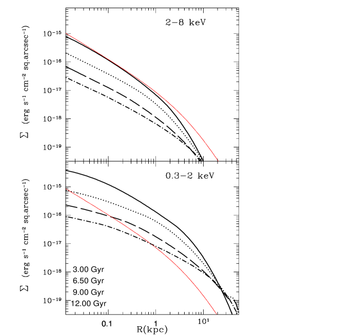
Figure 9: The X-ray surface brightness profiles of the hot gas for model B2${}_{02}\,$at quiescence, at the same times as for Fig. 7 (given in the bottom panel), for the hard band (upper panel) and the soft band (lower panel). The solid, dotted, dashed and dot-dashed lines correspond to increasing times. The red line follows the optical profile and shows the fiducial unresolved stellar emission due to low mass X-ray binaries, as would result from a long observation of a galaxy of the same luminosity $L_{\rm B}$ of the model (the line is normalized to give 20% of the total collective luminosity of these binaries, following the results for local ellipticals observed with $Chandra$, excluding the very hot gas rich ones, Boroson et al. 2011).

Figure 9 shows the evolution of the X-ray surface brightness profile of the gas $\Sigma(R)$ for B2${}_{02}\,$, at the same quiescent times of the temperature profiles in Fig. 7, for the soft (0.3-2 keV) and hard (2-8 keV) bands. In the hard band, $\Sigma(R)$ is always comparable to or lower than a profile representing the unresolved stellar emission due to low mass X-ray binaries, calculated for a deep (${\mathrel{\mathchoice{\lower 2.9pt\vbox{\halign{$\m@th\displaystyle\hfil#\hfil$\cr>\crcr\sim\crcr}}}{\lower 2.9pt\vbox{\halign{$\m@th\textstyle\hfil#\hfil$\cr>\crcr\sim\crcr}}}{\lower 2.9pt\vbox{\halign{$\m@th\scriptstyle\hfil#\hfil$\cr>\crcr\sim\crcr}}}{\lower 2.9pt\vbox{\halign{$\m@th\scriptscriptstyle\hfil#\hfil$\cr>\crcr\sim\crcr}}}}}200$ ksec) $Chandra$ pointing of a galaxy of the same optical luminosity as B2${}_{02}\,$and distant ${\mathrel{\mathchoice{\lower 2.9pt\vbox{\halign{$\m@th\displaystyle\hfil#\hfil$\cr<\crcr\sim\crcr}}}{\lower 2.9pt\vbox{\halign{$\m@th\textstyle\hfil#\hfil$\cr<\crcr\sim\crcr}}}{\lower 2.9pt\vbox{\halign{$\m@th\scriptstyle\hfil#\hfil$\cr<\crcr\sim\crcr}}}{\lower 2.9pt\vbox{\halign{$\m@th\scriptscriptstyle\hfil#\hfil$\cr<\crcr\sim\crcr}}}}}20$ Mpc. Thus, hard emission during quiescent times would be difficult to distinguish from the contribution of unresolved binaries, even with $Chandra$. In both bands $\Sigma(R)$ becomes flatter in shape with time increasing, since the emission level decreases mostly in the central galactic regions (within $R_{\rm e}$). This important effect is produced by the nuclear outbursts, that remove gas from the center.

In analogy with the discussion of the temperature profiles, Fig. 10 shows $\Sigma(R)$ just before, during, and after the last major nuclear burst at 7.498 Gyr, with times counted from the first accretion event. At -2 Myr the formation of the off-center cold shell produces the characteristic feature of a sharp decrease of $\Sigma$ in the hard band, and a bright rim in the soft band. The subsequent curves show the shock moving outwards after the major burst, and the presence of very hot gas at the center, revealed by the central peak in the hard band. The disturbances in the $\Sigma$ profiles due to the shells launched by the repeated sub-bursts are much more visible in the soft than in the hard band, as particularly apparent at +18 Myr. At this time, note the remarkable presence of a hot center surrounded by a denser and colder shell, producing a sharp peak in $\Sigma(R)$, at $R=600-700$ pc, and a sharp dip in $T_{\rm a}(R)$ in Fig. 8. The final two times (+66 Myr and +202 Myr) show the result of the degassing caused by the passage of the shock waves: the gas density is low, and subsonic perturbations remain at a radius of ${\mathrel{\mathchoice{\lower 2.9pt\vbox{\halign{$\m@th\displaystyle\hfil#\hfil$\cr>\crcr\sim\crcr}}}{\lower 2.9pt\vbox{\halign{$\m@th\textstyle\hfil#\hfil$\cr>\crcr\sim\crcr}}}{\lower 2.9pt\vbox{\halign{$\m@th\scriptstyle\hfil#\hfil$\cr>\crcr\sim\crcr}}}{\lower 2.9pt\vbox{\halign{$\m@th\scriptscriptstyle\hfil#\hfil$\cr>\crcr\sim\crcr}}}}}10$ kpc. A different representation of the profiles during the burst phases is given by Fig. 11, where $\Sigma_{\rm UM}(R)$ resulting from the unsharp masking procedure (Eq. 9) is shown. Fluctuations in brightness that can be clearly distinguished are that due to the cold shell (time -2 Myr), and, after the burst, the negative off-center region in $\Sigma_{\rm UM}(R)$ delimited by a sharp positive peak (times +6, +18, +66 Myr); the latter resembles what is commonly called a hot gas “cavity”.

Note that, when implemented in 2D simulations, the same input physics adopted for the present class of models gives conical hot gas outflows from the nucleus, during outbursts: hot gas is ejected along the symmetry axis, so that elongated ”cavities” (i.e., regions with a gas density decrement) are created (Novak et al. 2010). In addition, in their study of a model very similar to B3${}_{02}\,$, Jiang et al. (2010) found after a burst taking place at $6.5$ Gyr, a cavity filled with radio emitting particles of $\sim 4.4$ kpc in size, detectable during the first $\sim 10$ Myr after the burst. Therefore, we expect that cavities in the hot gas, such as those seen as off-center minima in the profiles of Figs. 10 and 11 at times from 6 to 66 Myr after the burst, should be fairly bright in the radio and would have, in X-rays, two essentially hollow conical lobes. They should even show non-thermal X-ray emission of the type seen in the Crab nebula (Jiang et al. 2010). Finally, taking at face value the results of the present analysis and the estimates on the radio detectability of Jiang et al. (2010), hot gas cavities seem more long-lasting than their radio detectability.

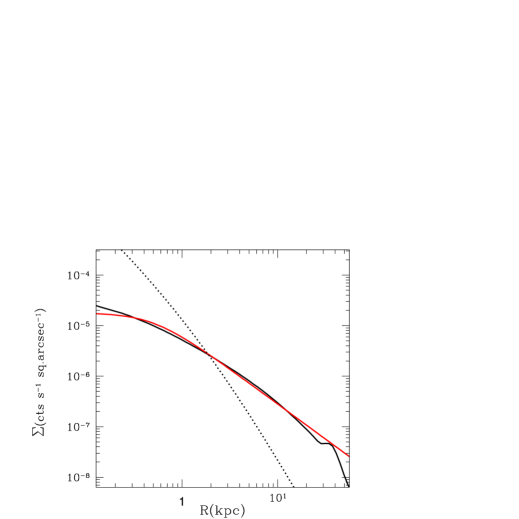
Figure 12: The 0.3–2 keV surface brightness profiles of the hot gas for B2${}_{02}\,$at an epoch of 9 Gyr (solid black line), compared with that of a model with the same $L_{\rm B}$, $\sigma$, $R_{\rm e}$ and $L_{\rm X}$ as B2${}_{02}\,$, but without feedback (dotted line); the conversion from flux to counts refers to a $Chandra$ ACIS pointing. Also shown is the best fit to the hot ISM brightness profile from an $Chandra$ ACIS pointing of the elliptical NGC4365 (at a distance of 20.4 Mpc), that has $L_{\rm B}$ and $L_{\rm X}$ close to that of the models (red, from Sarazin et al. 2003); the innermost flattening of the red profile within $\sim 200$ pc ($\sim 2^{\prime\prime}$) is due to PSF blurring effects.

Coming to the observability of the predicted features, one major property of the models is the decrease of $\Sigma(R)$ in the central galactic regions, produced by the nuclear outbursts, with respect to models without feedback. Interestingly, bright ellipticals imaged with $Chandra$ (e.g., Loewenstein et al. 2001) show a brightness profile that is quite flat within the central $\sim 1$ kpc, a feature impossible to reproduce with pure inflow models, while it resembles the profile of the “pre-burst” phase (black lines in Fig. 10, left panels), or at the end of a burst (+202 Myr). To better illustrate this point, Fig. 12 shows the different shape of $\Sigma(R)$ for B2${}_{02}\,$and for a model with the same $L_{\rm B}$, $\sigma$ and $R_{\rm e}$, but without AGN feedback, and the sole SNIa’s heating included. The two $\Sigma(R)$ profiles considered refer to the present quiescent epoch, yet the difference in steepness is clear. Figure 12 also shows the observed $\Sigma(R)$ for an elliptical at the periphery of the Virgo cluster, with $L_{\rm X}$ close to that of B2${}_{02}\,$; the agreement between model and observation is very good.

Another major prediction is given by the disturbances in the profile during an outburst; these keep above the level of the unresolved stellar emission, for a deep observation of a nearby galaxy with $Chandra$, as shown by Fig. 10. The central spike in $\Sigma(R)$, during the high-temperature and high-density phase at the center, is confined within $\sim 100$ pc, and then likely to remain a central unresolved feature even in galaxies observed at the high angular resolution of $Chandra$. Disturbances as shells and ripples farther out in the galaxy last ${\mathrel{\mathchoice{\lower 2.9pt\vbox{\halign{$\m@th\displaystyle\hfil#\hfil$\cr<\crcr\sim\crcr}}}{\lower 2.9pt\vbox{\halign{$\m@th\textstyle\hfil#\hfil$\cr<\crcr\sim\crcr}}}{\lower 2.9pt\vbox{\halign{$\m@th\scriptstyle\hfil#\hfil$\cr<\crcr\sim\crcr}}}{\lower 2.9pt\vbox{\halign{$\m@th\scriptscriptstyle\hfil#\hfil$\cr<\crcr\sim\crcr}}}}}0.2$ Gyrs, and are more likely to be observed. Given the typical duration of these features, and the presence of 3–4 major outbursts during the whole evolution, statistically they should be present, and possibly revealed by current X-ray observations, in $\simeq 5-10$% of the galaxies with $L_{\rm B}$ similar to the model galaxy.

In fact, many nearby galaxies show a disturbed appearance, as most recently revealed by studies based on $Chandra$ data (e.g., Finoguenov & Jones 2001, Forman et al. 2005, Soria et al. 2006, Diehl & Statler 2007, Nulsen et al. 2009, Baldi et al. 2009, Dunn et al. 2010). The ISM morphology of a large set of galaxies (54) shows a level of disturbance correlated with the radio luminosity derived by the NRAO VLA Sky Survey (thus including both pointlike and extended radio emission; Diehl & Statler 2008a). Also, many of the best studied gas-rich galaxies show decrements in the X-ray surface brightness map, identified as cavities formed when AGN jets inflate radio lobes and displace surrounding gas; in many cases the cavities are filled with radio plasma, and surrounded by armlike features, sometimes classified as shocks. The hot gas disturbances have then been generally attributed to jet activity. As discussed above, we expect that if we took two cones from our solutions, they would give ”lobes”. These would produce shocks at the edges and the lobes would be filled with radio emitting particles.

There are also a few galaxies without currently evident extended radio emission, but with signs of an outflow and hot central gas, as NGC4552 (Machacek et al. 2006). This galaxy shows a weak core radio source unresolved by the VLBA, and in the (unsharp masked) X-ray image two conspicuous ringlike features at 1.3 kpc from the galaxy center, surrounding two cavities; these features have been found consistent with shocked gas driven outward by recent nuclear activity, as in a bipolar nuclear outflow. The gas temperature in the central $\sim 100$ pc of the galaxy is $1\pm 0.2$ keV, hotter than elsewhere in the galaxy, suggesting that we may be directly observing the reheating of the galaxy ISM by the outburst (Machacek et al. 2006). These characteristics resemble those predicted by the models for the temperature and the surface brighntess during the afterburst phase.

7 Discussion and conclusions

The hot gas properties of massive ellipticals, with regard to luminosity and temperature, and their spatial distributions, allow us to derive insights into the hot gas evolutionary status, and its link with the host galaxy. Since the cooling times are short compared to the galaxy age, it is now commonly accepted that repeated cooling catastrophes have occurred in the past, accompanied by central starbursts and AGN outbursts. The interest of a better understanding of this phenomenon is obvious, as it is directly linked to galaxy formation and evolution, and to the growth of the central MBH. Unfortunately, a complete theoretical picture is still missing, so that modeling coupled with a close comparison with observations is crucial in this field. In fact, these feedback events must leave signatures on the X-ray properties of the galaxies; indeed, the observed temperature and brightness profiles often cannot be fit easily with smooth profiles, or cooling flow profiles (e.g., Sarazin 2011, Statler 2011). In this work we have calculated the observational properties in the X-ray band of two galaxy models, representative of a class of detailed simulations of physically based models for the investigation of feedback modulated accretion in isolated galaxies. The feedback physics includes the combined effects of radiation and AGN winds (Paper III). The observational properties derived provide good matches to what observed in general for the local universe, and account for a few otherwise puzzling observed properties; on the other hand, they also evidence the need for changes or additions to the input physics. The main results of the present investigation are the following:

1) After an evolution of $\simeq 10$ Gyr, the models are typically in a permanent quiescent phase. The bolometric nuclear emission is very sub-Eddington ($l\simeq 10^{-4}$), within the range observed for $l$, though the most frequently observed values ($l\approx 10^{-5}$ or less) are somewhat lower. Unfortunately, uncertainties in the bolometric correction to apply to observed nuclear luminosities, appropriate for a spectral energy distribution at low emission levels, do not allow to make a stringent comparison between modelled and observed values. However, also the nuclear X-ray emission $L_{\rm BH,X}$ of the models, estimated as $L_{\rm BH,X}{\mathrel{\mathchoice{\lower 2.9pt\vbox{\halign{$\m@th\displaystyle\hfil#\hfil$\cr<\crcr\sim\crcr}}}{\lower 2.9pt\vbox{\halign{$\m@th\textstyle\hfil#\hfil$\cr<\crcr\sim\crcr}}}{\lower 2.9pt\vbox{\halign{$\m@th\scriptstyle\hfil#\hfil$\cr<\crcr\sim\crcr}}}{\lower 2.9pt\vbox{\halign{$\m@th\scriptscriptstyle\hfil#\hfil$\cr<\crcr\sim\crcr}}}}}0.2L_{\rm BH}$ as should be appropriate for low luminosity nuclei, and $L_{\rm BH,X}/L_{\rm Edd}$, tend to lie on the upper end of what is observed. Thus in real galaxies an additional mechanism may be required to reduce further the mass available for accretion; this could be provided by the mechanical feedback of a (nuclear) jet, and/or by a thermally driven wind from a RIAF. Alternatively, the switch from disc to RIAF behavior (that is $l\propto\dot{m}^{2}$) should occur at a larger $l$ than assumed here (e.g., at $l\simeq 0.1$ rather than $l\simeq 0.01$). Simulations of ram-pressure stripping effects, instead, showed that a reduction in the accretion rate is not attained, because in the quiescent hot accretion regime, the accreting mass comes mainly from the stellar mass losses within the central $\sim 100$ parsecs of the galaxy, that are not affected by stripping (Shin et al. 2010b).

2) The X-ray luminosity of the ISM oscillates in phase with the nuclear luminosity, though with much broader peaks; at the present epoch, $L_{\rm X}$ lies at the lower end of the large observed range for galaxies of $L_{\rm B}$ similar to that of the models. The degassing/heating in the models may then be too efficient, or a larger/more concentrated gravitating mass, or a confining external medium, are needed. However, when the gas luminosities during the whole evolution are considered, the observed $L_{\rm X}$ range is better reproduced. This is even more true if also an additional model of larger $\sigma$, and same $L_{\rm B}$, is included. Part of the observed large variation in $L_{\rm X}$ for galaxies of a given $L_{\rm B}$ could then be explained by nuclear activity.

3) The average ISM temperature is within the observed large range for the model $\sigma$; when estimated within $R_{\rm e}$, the model temperatures reproduce better the upper half of those observed. Modifications to the models by the addition of a jet or an external medium, as suggested in the previous points, should then not increase the average temperature within $R_{\rm e}$.

4) During quiescence, the profiles of the gas temperature and brightness resemble those observed for many local galaxies. Especially remarkable is the lack of the steep brightness profile shape typical of inflowing models, due to the frequent removal of gas from the galactic central regions, and to the heating provided by mechanical feedback (that is always present, even during quiescent phases). The models show negative temperature gradients, that are common for isolated galaxies; the addition of a jet or a confining agent should change the temperature profiles into a flat or outwardly increasing profile, as also frequently observed for galaxies in rich environments.

5) During outbursts, disturbances are predicted in the temperature and brightness profiles; the ISM resumes the smooth appearance of steady and low-luminosity hot accretion on the MBH on a time-scale of ${\mathrel{\mathchoice{\lower 2.9pt\vbox{\halign{$\m@th\displaystyle\hfil#\hfil$\cr<\crcr\sim\crcr}}}{\lower 2.9pt\vbox{\halign{$\m@th\textstyle\hfil#\hfil$\cr<\crcr\sim\crcr}}}{\lower 2.9pt\vbox{\halign{$\m@th\scriptstyle\hfil#\hfil$\cr<\crcr\sim\crcr}}}{\lower 2.9pt\vbox{\halign{$\m@th\scriptscriptstyle\hfil#\hfil$\cr<\crcr\sim\crcr}}}}}200$ Myrs. The most conspicuous variations with respect to smooth profiles are within current detection capabilities, and could correspond to (part of) the widespread disturbances observed in galaxies of the local Universe. In particular, shocked hot gas should be seen at the galactic center (within $\sim 100$ pc), possibly not resolved; this would be a certain sign of prior AGN activity. These hot bubbles could be revealed by emission of cosmic-rays, in a structure similar to a gigantic supernova remnant. Preliminary results from 2D runs show bipolar nuclear outflows, that should be seen as conical cavities extending from the galactic center, and may be called jet-like features.

6) The duty-cycle of nuclear activity is of the order of a few $\times(10^{-3}-10^{-2})$, depending on the assumed mechanical feedback efficiency; in general, a burst cycle lasts for $\approx 10^{7}$ yrs. These duty-cycle values are broadly consistent with the fraction of active galaxies measured in observational works, though reported values for the local universe are somewhat lower, for the MBH mass of the models. In order to make a more consistent comparison with observations, the dataset of models should be increased, and the duty cycle computed only for the last 2–3 Gyrs; this will reduce the duty cycle, as the models are characterized by a declining nuclear activity.

7) The duty-cycle of perturbances in the ISM is of the order of 5-10%, from their average number and duration. This duty-cycle likely increases with galaxy mass, because an outburst has a greater impact in less massive (and less gas-rich) systems, which then are ”on” for a shorter time (Ciotti & Ostriker 2011). The ISM duty-cycle, and its trend with galaxy mass, compare reasonably well with preliminary estimates obtained from a large sample of hot gas coronae in elliptical galaxies observed with $Chandra$ (Nulsen et al. 2009): the fraction of galaxies with X-ray cavities in the hot gas is ${\mathrel{\mathchoice{\lower 2.9pt\vbox{\halign{$\m@th\displaystyle\hfil#\hfil$\cr<\crcr\sim\crcr}}}{\lower 2.9pt\vbox{\halign{$\m@th\textstyle\hfil#\hfil$\cr<\crcr\sim\crcr}}}{\lower 2.9pt\vbox{\halign{$\m@th\scriptstyle\hfil#\hfil$\cr<\crcr\sim\crcr}}}{\lower 2.9pt\vbox{\halign{$\m@th\scriptscriptstyle\hfil#\hfil$\cr<\crcr\sim\crcr}}}}}10$% when $L_{\rm X}<10^{41}$ erg s^-1 (as for the models), and reaches $\sim 25$% in the most luminous ones. The presence of cavities has been attributed to the action of jets inflating radio lobes and displacing the surrounding gas. Cavities can also be created in the scenario presented here, as hinted for by 2D simulations, due to bipolar nuclear outflows.

7) Two diagnostic planes have been constructed. In the first one, the nuclear luminosity $L_{\rm BH}$ and the ISM luminosity $L_{\rm X}$ are followed during the whole model evolution. The points representative of the models populate a wedge region, that should then be occupied when observing a large set of galaxies. Another plane shows the evolution of $L_{\rm X}$ versus the average gas temperature $T_{\rm a}$; here the most populated region is that of a large $L_{\rm X}$ variation (factor of $\sim 10$) for $T_{\rm a}$ keeping between 0.4 and 0.6 keV.

Clearly, a larger set of models is to be explored, in order to better establish the final gas properties (as gas content, nuclear and ISM duty-cycle, etc.) to be compared with those of a statistically large sample. For example, a general expectation is that changes of the galaxy properties have an impact on the number of nuclear outbursts: depending on many model parameters (supernova rate, central $\sigma$, dark matter amount and distribution, and even external pressure due to an intragroup or intracluster medium), bursts could take place even towards the present epoch, or be confined to the early epoch (Ciotti & Ostriker 2011).

Table 1: The representative models

Model	$\epsilon_{\rm w}^{\rm M}$	$<\epsilon_{\rm w}>$	$<\epsilon_{\rm EM}>$	$\log\Delta M_{\rm BH}$	$\log\Delta M_{*}$	$\log\Delta M_{\rm w}$	$\log M_{\rm gas}$	$\log L_{\rm BH,opt}^{\rm eff}/L_{\rm Edd}$
(1)	(2)	(3)	(4)	(5)	(6)	(7)	(8)	(9)
B2${}_{02}\,$	$10^{-3}$	$2.0\,10^{-5}$	0.105	8.74	9.74	10.27	9.68	-5.13
B3${}_{02}\,$	$3\times 10^{-4}$	$1.2\times 10^{-5}$	0.133	9.05	10.22	10.31	9.34	-5.43

Table 2: Nuclear and gas emission properties (at 12 Gyr)

Model	$M_{\rm BH}$	log$L_{\rm BH}$	$l$	$L_{\rm BH,X}$	$L_{\rm BH,X}/L_{Edd}$		duty cycle		$\log L_{\rm X}$
	($M_{\odot}$)	(erg s-1)	($10^{-4}$)	(erg s-1)		Bol	Opt	UV	(erg s-1)
(1)	(2)	(3)	(4)	(5)	(6)	(7)	(7)	(7)	(8)
B2${}_{02}\,$	$8.4\times 10^{8}$	43.39	2.0	${\mathrel{\mathchoice{\lower 2.9pt\vbox{\halign{$\m@th\displaystyle\hfil#\hfil$\cr<\crcr\sim\crcr}}}{\lower 2.9pt\vbox{\halign{$\m@th\textstyle\hfil#\hfil$\cr<\crcr\sim\crcr}}}{\lower 2.9pt\vbox{\halign{$\m@th\scriptstyle\hfil#\hfil$\cr<\crcr\sim\crcr}}}{\lower 2.9pt\vbox{\halign{$\m@th\scriptscriptstyle\hfil#\hfil$\cr<\crcr\sim\crcr}}}}}5\times 10^{42}$	${\mathrel{\mathchoice{\lower 2.9pt\vbox{\halign{$\m@th\displaystyle\hfil#\hfil$\cr<\crcr\sim\crcr}}}{\lower 2.9pt\vbox{\halign{$\m@th\textstyle\hfil#\hfil$\cr<\crcr\sim\crcr}}}{\lower 2.9pt\vbox{\halign{$\m@th\scriptstyle\hfil#\hfil$\cr<\crcr\sim\crcr}}}{\lower 2.9pt\vbox{\halign{$\m@th\scriptscriptstyle\hfil#\hfil$\cr<\crcr\sim\crcr}}}}}2\times 10^{-5}$	$6.3\times 10^{-3}$	$3.2\times 10^{-3}$	$3.0\times 10^{-3}$	40.1
B3${}_{02}\,$	$1.4\times 10^{9}$	43.38	1.0	${\mathrel{\mathchoice{\lower 2.9pt\vbox{\halign{$\m@th\displaystyle\hfil#\hfil$\cr<\crcr\sim\crcr}}}{\lower 2.9pt\vbox{\halign{$\m@th\textstyle\hfil#\hfil$\cr<\crcr\sim\crcr}}}{\lower 2.9pt\vbox{\halign{$\m@th\scriptstyle\hfil#\hfil$\cr<\crcr\sim\crcr}}}{\lower 2.9pt\vbox{\halign{$\m@th\scriptscriptstyle\hfil#\hfil$\cr<\crcr\sim\crcr}}}}}5\times 10^{42}$	${\mathrel{\mathchoice{\lower 2.9pt\vbox{\halign{$\m@th\displaystyle\hfil#\hfil$\cr<\crcr\sim\crcr}}}{\lower 2.9pt\vbox{\halign{$\m@th\textstyle\hfil#\hfil$\cr<\crcr\sim\crcr}}}{\lower 2.9pt\vbox{\halign{$\m@th\scriptstyle\hfil#\hfil$\cr<\crcr\sim\crcr}}}{\lower 2.9pt\vbox{\halign{$\m@th\scriptscriptstyle\hfil#\hfil$\cr<\crcr\sim\crcr}}}}}2\times 10^{-5}$	$4.8\times 10^{-2}$	$1.8\times 10^{-2}$	$8.6\times 10^{-3}$	39.6

Figure 1: Time evolution of the nuclear luminosity for models B2${}_{02}\,$(upper panel) and B3${}_{02}\,$(bottom panel). The Eddington luminosity $L_{\rm Edd}$ (the almost horizontal solid line), and the bolometric luminosity resulting from accretion on the MBH, $L_{\rm BH}=\epsilon\dot{M}_{\rm BH}c^{2}$ (dotted line), are shown. The larger number of bursts shown by B3${}_{02}\,$, their larger temporal extension and substructure, are due to the reduced peak value of mechanical efficiency $\epsilon_{\rm w}^{\rm M}$ of the AGN wind (see Sect. 2). The bursts become rarer for increasing time, in pace with the decreasing mass return rate from the evolving stellar population.

Figure 5: The total gas emission versus the aperture temperature (within $10R_{\rm e}$), calculated for the 0.3-8 keV band, for model B2${}_{02}\,$. As for Fig. 4, the time evolution from 2 to 14 Gyrs corresponds to the increasing numbers along the curve; the time sampling is uniform, with time steps of 50 Myr.

Figure 6: Normalized histogram (dotted lines) of the 0.3–8 keV emission weighted temperature $T_{\rm a}(R_{\rm e})$, during the epoch from 2 to 12 Gyrs, for the model indicated in each panel; the histograms are calculated as for Fig. 3. The histograms of the models are compared with that derived for $T_{\rm a}(R_{\rm e})$ from $Chandra$ data (Athey 2007), for a subsample of 20 ellipticals in the log$L_{B}$ range from 10.5 to 10.8 (solid line). See Sect. 5.2.

Figure 7: Left panel: radial profile of the 0.3–8 keV emission-weighted projected temperature $T_{\rm p}(R)$ (Eq. 5), during the interburst times indicated in the panel, for model B2${}_{02}\,$. The temperature increases with time, due to the secular increase of the ISM specific heating, and the growing MBH mass, which modifies the local gravitational field and the central stellar velocity dispersion (see Sect. 6.1 for more details). The sharp drop in the red and green profiles at $\approx 40$ kpc is due to disturbances produced by the outbursts at 5.5 and 7.5 Gyr (Fig. 1) that are still traveling outward. Right panel: the corresponding aperture temperature profiles $T_{\rm a}(R)$, obtained from averaging $T_{\rm p}(R)$ using the surface brightness (Eq. 6). The bin-width increases going outward in the galaxy, to reproduce the best observed profiles of nearby galaxies.

References

- (1)
- (2) Athey, A.E. 2007, PhD thesis, arXiv:0711.0395
- (3)
- (4) Baldi, A., Forman, W., Jones, C., et al. 2009, ApJ 707, 1034
- (5)
- (6) Blandford, R., Begelman, M.C. 1999, MNRAS303, L1
- (7)
- (8) Benson, A.J., & Babul, A. 2009, MNRAS, 397, 1302
- (9)
- (10) Bondi, H. 1952, MNRAS, 112, 195
- (11)
- (12) Boroson, B., Kim, D.W., Fabbiano, G., 2011, ApJ 729, 12
- (13)
- (14) Brighenti, F., Mathews, W.G., 1998, ApJ, 495, 239
- (15)
- (16) Brown, B. A., Bregman J. N., 2000, ApJ, 539, 592
- (17)
- (18) Cattaneo, A., et al., 2009, Nature, 460, 213
- (19)
- (20) Chartas, G., Brandt, W. N., Gallagher, S. C. 2003, ApJ 595, 85
- (21)
- (22) Ciotti, L., D’Ercole, A., Pellegrini, S., & Renzini, A., 1991, ApJ, 376, 380
- (23)
- (24) Ciotti, L., Morganti, L., deZeeuw, P.T., 2009, MNRAS, 393, 491
- (25)
- (26) Ciotti, L., & Ostriker, J.P., 1997, ApJ, 487, L105
- (27)
- (28) Ciotti, L., & Ostriker, J.P., 2001, ApJ, 551, 131
- (29)
- (30) Ciotti, L., & Ostriker, J.P. 2007, ApJ 665, 1038
- (31)
- (32) Ciotti, L., & Ostriker, J.P. 2011, in Hot Interstellar Matter in Elliptical Galaxies, eds. D.W Kim and S. Pellegrini, Springer ASSL Series, Springer (New York, NY, USA), in press.
- (33)
- (34) Ciotti, L., Ostriker, J.P., Proga, D., 2009, ApJ, 699, 89 (Paper I)
- (35)
- (36) Ciotti, L., Ostriker, J.P., Proga, D., 2010, ApJ, 717, 708 (Paper III)
- (37)
- (38) Ciotti, L., Pellegrini, S. 2008, MNRAS, 387, 902
- (39)
- (40) Crenshaw, D.M., Kraemer, S.B., George, I. M. 2003, ARAA 41, 117
- (41)
- (42) David, L. P., Forman, W., Jones, C., 1991, ApJ 369, 121
- (43)
- (44) Diehl, S., Statler, T.S. 2007, ApJ 668, 150
- (45)
- (46) Diehl, S., Statler, T.S. 2008a, ApJ 680, 897
- (47)
- (48) Diehl, S., Statler, T.S. 2008b, ApJ 687, 986
- (49)
- (50) Di Matteo, T., Springel, V., Hernquist, L. 2005, Nature 433, 604
- (51)
- (52) Dunn, R. J. H., Allen, S. W., Taylor, G. B., et al. 2010, MNRAS 404, 180
- (53)
- (54) Fabbiano, G., 1989, ARA&A, 27, 87
- (55)
- (56) Fabbiano, G. 2011, in Hot Interstellar Matter in Elliptical Galaxies, eds. D.W. Kim and S. Pellegrini, Springer ASSL Series, Springer (New York, NY, USA), in press.
- (57)
- (58) Fabbiano, G.; Kim, D.-W.; Trinchieri, G., 1992, ApJS 80, 531
- (59)
- (60) Fabian, A.C., & Canizares, C.R. 1988, Nature 333, 829
- (61)
- (62) Fabian, A. C., Sanders, J. S., Allen, S. W., et al. 2003, MNRAS, 344, L43
- (63)
- (64) Ferrarese, L., Merritt, D. 2000, ApJ, 539, L9
- (65)
- (66) Finoguenov, A., Jones, C., 2001, ApJ, 547, L107
- (67)
- (68) Forman, W., Nulsen, P., Heinz, S., et al. 2005, ApJ, 635, 894
- (69)
- (70) Fukazawa, Y., Botoya-Nonesa, J. G., Pu, J., Ohto, A., Kawano, N. 2006, ApJ 636, 698
- (71)
- (72) Gallo, E., Treu, T., Marshall, P.J., Woo, J.-H., Leipski, C., Antonucci, R. 2010, ApJ 714, 25
- (73)
- (74) Gebhardt, K., et al. 2000, ApJ, 539, L13
- (75)
- (76) Graham, A.W., Erwin, P., Caon, N., & Trujillo, I. 2001, ApJ, 563, L13
- (77)
- (78) Greene, Jenny E., Ho, Luis C., 2007, ApJ 667, 131
- (79)
- (80) Grevesse, N.; Sauval, A. J., 1998, Space Science Reviews, v. 85, p. 161-174
- (81)
- (82) Haiman, Z., Ciotti, L., Ostriker, J.P. 2004, ApJ 606, 763
- (83)
- (84) Heckman, T.M., Kauffmann, G., Brinchmann, J., Charlot, S., Tremonti, C., White, S.D.M., 2004, ApJ, 613, 109
- (85)
- (86) Helsdon, S.F., Ponman, T.J., O’Sullivan, E., Forbes, D.A., 2001, MNRAS, 325, 693
- (87)
- (88) Ho, L. C. 2008, ARAA 46, 475
- (89)
- (90) Ho, L. C., 2009, ApJ 699, 626
- (91)
- (92) Hopkins, P.F., Hernquist, L., Cox, T.J., Roberston, B., Di Matteo, T., Springel, V., 2005, ApJ, 625, L71
- (93)
- (94) Hopkins, P.F., Hernquist, L., Cox, T.J., Di Matteo, T., Robertson, B., Springel, V. 2006, ApJS 163, 1
- (95)
- (96) Humphrey, P.J., Buote, D. A., Gastaldello, F., et al. 2006, ApJ 646, 899
- (97)
- (98) Jaffe, W., 1983, MNRAS, 202, 995
- (99)
- (100) Jiang, Y.-F., Ciotti, L., Ostriker, J.P., Spitkovsky, A., 2010, ApJ, 711, 125
- (101)
- (102) Johansson, P.H., Naab, T., Burkert, A., 2009, ApJ, 690, 802
- (103)
- (104) Jones, C., Forman, W., Vikhlinin, A., Markevitch, M., David, L., Warmflash, A., Murray, S., Nulsen, P. E. J., 2002, ApJ 567, L115
- (105)
- (106) Kim, D.W., Fabbiano, G., 2003, ApJ, 586, 826
- (107)
- (108) Kormendy, J., Fisher, D.B., Cornell, M.E., Bender, R., 2009, ApJS, 182, 216
- (109)
- (110) Loewenstein, M., Davis, D.S., 2010, ApJ 716, 384
- (111)
- (112) Loewenstein, M., Mushotzky, R.F., Angelini, L., Arnaud, K.A., Quataert, E., 2001, ApJ 555, L21
- (113)
- (114) Machacek, M., Nulsen, P.E.J., Jones, C., Forman, W. R., 2006, ApJ 648, 947, 2006.
- (115)
- (116) Magorrian, J., et al. 1998, AJ, 115, 2285
- (117)
- (118) Mahadevan, R. 1997, ApJ 477, 585.
- (119)
- (120) Matsushita, K., 2001, ApJ, 547, 693
- (121)
- (122) Merloni, A., Rudnick, G., Di Matteo, T., 2004, MNRAS 354, L37
- (123)
- (124) Million, E.T., Werner, N., Simionescu, A., et al., 2010, MNRAS 407, 2046
- (125)
- (126) Mulchaey, J. S., Jeltema, T. E., 2010, ApJ 715, L1
- (127)
- (128) Nagino, R., Matsushita, K., 2009, A&A, 501, 157
- (129)
- (130) Narayan, R., Yi, I., 1994, ApJ 428, L13
- (131)
- (132) Novak, G.S., Ostriker, J.P., Ciotti, L., 2010, accepted by ApJ (arXiv:1007.3505)
- (133)
- (134) Nulsen, P., Jones, C., Forman, W., et al. 2009, AIPC 1201, 198
- (135)
- (136) Ostriker, J. P., Ciotti, L., 2005, RSPTA 363, 667
- (137)
- (138) Ostriker, J.P., Choi, E., Ciotti, L., Novak, G.S., Proga, D., 2010, ApJ 722, 642
- (139)
- (140) O’Sullivan, E., Forbes, D., Ponman, T. 2001, MNRAS 328, 461
- (141)
- (142) O’Sullivan, E., Ponman, T.J., Collins, R.S., 2003, MNRAS 340, 1375
- (143)
- (144) O’Sullivan, E., Vrtilek, J.M., Harris, D.E., Ponman, T.J., 2007, ApJ 658, 299
- (145)
- (146) Pellegrini, S., Ciotti, L., 1998, A&A 333, 433
- (147)
- (148) Pellegrini, S., 2005, ApJ 624, 155
- (149)
- (150) Pellegrini, S., Baldi, A., Kim, D.W., Fabbiano, G., Soria, R., Siemiginowska, A., Elvis, M., 2007, ApJ 667, 731
- (151)
- (152) Pellegrini, S., Ciotti, L., Ostriker, J.P., 2009, Adv. Space Res., 44, 340
- (153)
- (154) Pellegrini, S., 2010, ApJ 717, 640
- (155)
- (156) Pellegrini, S., 2011, accepted by ApJ (arXiv:1106.2898)
- (157)
- (158) Pellegrini, S., 2011, in Hot Interstellar Matter in Elliptical Galaxies, eds. D.W. Kim and S. Pellegrini, Springer ASSL Series, Springer (New York, NY, USA), in press.
- (159)
- (160) Peterson, J. R., Fabian, A. C., 2006, Physics Reports, 427, 1
- (161)
- (162) Proga, D., 2003, ApJ 585, 406
- (163)
- (164) Proga, D., & Kallman, T. 2004, ApJ, 616, 688
- (165)
- (166) Proga, D., Stone, J.M., & Kallman, T. 2000, ApJ, 543, 686
- (167)
- (168) Renzini, A., Ciotti, L., D’Ercole, A., Pellegrini, S., ApJ, 1993, 419, 52
- (169)
- (170) Sansom, A. E., O’Sullivan, E., Forbes, D. A., Proctor, R. N., Davis, D. S. 2006, MNRAS 370, 1541
- (171)
- (172) Sarazin, C.L., 2011, in Hot Interstellar Matter in Elliptical Galaxies, eds. D.W. Kim and S. Pellegrini, Springer ASSL Series, Springer (New York, NY, USA), in press.
- (173)
- (174) Sarazin, C.L., White, R.E.III, 1987, ApJ, 320, 32
- (175)
- (176) Sazonov, S.Yu., Ostriker, J.P., Ciotti, L., & Sunyaev, R.A., 2005, MNRAS, 358, 168
- (177)
- (178) Schawinski, K., Lintott, C. J., Thomas, D., et al. 2009, ApJ 690, 1672
- (179)
- (180) Shin, M.S., Ostriker, J.P., Ciotti, L., 2010a, ApJ, 711, 268
- (181)
- (182) Shin, M.S., Ostriker, J.P., Ciotti, L., 2010b, submitted to ApJ (arXiv:1003:1108)
- (183)
- (184) Silk, J., Rees, M. J. 1998, A&A 331, L1
- (185)
- (186) Smith, R.K., Brickhouse, N.S., Liedahl, D.A., Raymond, J.C. 2001, ApJ 556, L91
- (187)
- (188) Soltan, A., 1982, MNRAS 200, 115
- (189)
- (190) Somerville, R.S., Hopkins, P.F., Cox, T.J., Robertson, B.E., Hernquist, L. 2008, MNRAS 391, 481
- (191)
- (192) Soria, R., Fabbiano, G., Graham, A., Baldi, A., Elvis, M., Jerjen, H., Pellegrini, S., Siemiginowska, A. 2006, ApJ 640, 126
- (193)
- (194) Statler, T., 2011, in Hot Interstellar Matter in Elliptical Galaxies, eds. D.W. Kim and S. Pellegrini, Springer ASSL Series, Springer (New York, NY, USA), in press.
- (195)
- (196) Trinchieri, G., Pellegrini, S., Fabbiano, G., et al., 2008, ApJ, 688, 1000
- (197)
- (198) Vedder, P.W., Trester, J.J., Canizares, C.R. 1988, ApJ 332, 725
- (199)
- (200) White, R. E., III, Sarazin, C. L., 1991, ApJ 367, 476
- (201)
- (202) Yan, R., Newman, J. A., Faber, S. M., Konidaris, N., Koo, D., Davis, M. 2006, ApJ 648, 281
- (203)
- (204) Yu, Q., Tremaine, S. 2002, MNRAS 335, 965
- (205)