The luminosities of the brightest cluster galaxies and brightest satellites in SDSS groups

Abstract

We show that the distribution of luminosities of Brightest Cluster Galaxies in an SDSS-based group catalog suggests that BCG luminosities are just the statistical extremes of the group galaxy luminosity function. This latter happens to be very well approximated by the all-galaxy luminosity function (restricted to $M_{r}<-19.9$), provided one uses a parametrization of this function that is accurate at the bright end. A similar analysis of the luminosity distribution of the Brightest Satellite Galaxies suggests that they are best thought of as being the second brightest pick from the same luminosity distribution of which BCGs are the brightest. I.e., BSGs are not the brightest of some universal satellite luminosity function, in contrast to what Halo Model analyses of the luminosity dependence of clustering suggest. However, we then use mark correlations to provide a novel test of these order statistics, showing that the hypothesis of a universal luminosity function (i.e. no halo mass dependence) from which the BCGs and BSGs are drawn is incompatible with the data, despite the fact that there was no hint of this in the BCG and BSG luminosity distributions themselves. We also discuss why, since extreme value statistics are explicitly a function of the number of draws, the consistency of BCG luminosities with extreme value statistics is most clearly seen if one is careful to perform the test at fixed group richness $N$. Tests at, e.g., fixed total group luminosity $L_{\rm tot}$, will generally be biased and may lead to erroneous conclusions.

1 Introduction

The study of whether or not the brightest cluster galaxy (the BCG) is special, rather than simply being the brightest by chance, has a long history (Scott 1957; Schechter & Peebles 1976; Tremaine & Richstone 1977; Bhavsar & Barrow 1985; Loh & Strauss 2006; Lin, Ostriker & Miller 2010, Dobos & Csabai 2011). Since the BCG is usually at or close to the cluster center, it is plausible that its formation history was dominated by different physical processes compared to the other galaxies in the cluster, which we will call satellites. For this reason, models of BCG formation routinely assume that BCGs are special (e.g. Milosavljević, et al. 2006; De Lucia & Blaizot 2007). And there is growing evidence from scaling relations that BCGs are indeed special: they have larger sizes, smaller velocity dispersions, smaller color gradients, and are less spherical than expected for their luminosities (e.g. Bernardi et al. 2011). But whether or not this has left a distinct signature in the distribution of BCG luminosities is an open question.

There are at least two reasons why the answer is interesting. First, Halo Model (see Cooray & Sheth 2002 for a review) interpretations of the luminosity dependence of galaxy clustering explicitly distinguish between the central and the other (satellite) galaxies in a halo. If BCGs are just the brightest of a universal galaxy luminosity function, then including this constraint significantly simplifies such analyses.

The second is that the distribution of BCG luminosities is considerably narrower than that of all galaxies, so the large number of clusters that will soon be available may permit BCGs to provide a useful consistency check of standard candle constraints on the luminosity-distance relation (Hubble 1936; Scott 1957; Sandage, Kristian & Westphal 1976). Alternatively, if the $d_{\rm L}(z)$ relation is known and BCGs are just statistical extremes, then the BCG luminosity function can be used to provide a rather accurate determination of the evolution of the galaxy luminosity function. Since BCGs are bright, they are amongst the easiest targets for spectroscopy, so this measure of galaxy evolution comes at a small fraction of the cost of a full galaxy survey. On the other hand, if they are special in other ways, one must also understand how the physical processes which affected their formation evolve.

In what follows we will use the Halo Model analyses to motivate why one might have thought that the BCG luminosity function might simply be given by the extreme value statistics of the all galaxy luminosity function, even though centrals are often explicitly treated as being special. In this case, it is natural to ask if the luminosity function of the brightest satellite galaxies – the BSG luminosity function – is simply given by the associated order statistics of the second brightest (rather than the brightest) object. Then we will show that Halo Model analyses also suggest that the BSG luminosity function should be given by the extreme value statistics of a satellite galaxy luminosity function, rather than the order statistics of the all galaxy luminosity function. We will show that both statements cannot be right, so we turn to the data to decide the issue.

Section 2 summarizes the main results from Order Statistics and the Halo Model approach which are relevant to this study. Section 3 uses a group catalog of SDSS galaxies from Berlind et al. (2006) (henceforth B06) to test these models regarding BCGs and BSGs. These tests include the luminosity functions of BCGs and BSGs, the ratio of the luminosities of the first and second brightest galaxies in a cluster, and the luminosity function of satellite galaxies (i.e., not just the BSGs). Section 4 shows that luminosity weighted clustering provides a novel test of Order Statistics. A final section summarizes. Appendix A provides a derivation of the satellite distribution if the BCGs satisfy extreme value statisics. Appendix B demonstrates that tests of order statistics are better made holding the number of galaxies fixed, rather than other parameters such as group luminosity, etc. And Appendix C describes the details of the Halo Model that are relevant to our study.

2 Preliminaries

2.1 Extreme value and order statistics

The probability that the largest of $N$ independent draws from a distribution $p(L)$ is less than $L$ is given by

$$g_{1}(<L|N)=P(<L)^{N}\,,$$ (1)

where $P(<L)=\int_{L_{\rm min}}^{L}{\rm d}L^{\prime}p(L^{\prime})$, and we will define the value of $L_{\rm min}$ later. The associated differential distribution is

$$g_{1}(L|N)=N\,p(L)\,P(<L)^{N-1}\,.$$ (2)

Similarly, the distribution of the second largest of the $N$ draws satisfies

$$g_{2}(<L|N)=P(<L)^{N}+{N\choose 1}\,P(>L)\,P(<L)^{N-1}\,,$$ (3)

so that

$$g_{2}(L|N)=N(N-1)\,p(L)\,P(>L)\,P(<L)^{N-2}\,.$$ (4)

More generally, the $n$th largest of $N$ draws obeys

$$g_{n}(L|N)={N\choose n}\,np(L)\,P(>L)^{n-1}\,P(<L)^{N-n}\,.$$ (5)

In what follows we will be interested in whether or not the distribution of BCG and BSG luminosities are given by equations (2) and (4) respectively, with $p(L)$ given by the luminosity function of all galaxies, although clearly, similar tests with the other values of $n$ could also be devised.

If we define the satellite luminosity function as the distribution which is obtained by subtracting the distribution of centrals (assumed to be $g_{1}(>L|N)$) from that of all galaxies, then one might ask if the luminosity function of BSGs is given by inserting this distribution of satellite luminosities for $p$ in the expression above for $g_{1}$. In Appendix A, we show that this is not the same as $g_{2}$. We will argue shortly that the Halo Model suggests that both of these models might be acceptable for satellites.

When discussing the group catalog of B06, we will use the luminosity distribution $p_{\rm gal}(L)$ derived from equation (9) of Bernardi et al. (2010), restricted and normalized to $L>L_{\rm min}$, for some $L_{\rm min}$ which we will specify shortly. Explicitly,

$$L\,p_{\rm gal}(L)=\frac{\beta\,(L/L_{\ast})^{\alpha}\,{\rm e}^{-(L/L_{\ast})^{\beta}}}{\Gamma\left(\alpha/\beta,(L_{\rm min}/L_{\ast})^{\beta}\right)}.$$ (6)

The parameters in Table B1 of Bernardi et al. assumed that absolute magnitudes brighten as $1.3z$, and were quoted at $z=0$. Since the B06 sample is based on absolute magnitudes that were $k$-corrected and evolution corrected to $z=0.1$, we adopt an increased value $L_{\ast}$ (by a factor $10^{0.4\times 1.3\times 0.1}$) but leave the other parameters $\alpha$ and $\beta$ unchanged. I.e., we use,

$$L_{\ast}=0.104\times 10^{10}L_{\odot}h^{-2}~{};~{}\alpha=1.12~{};~{}\beta=0.533\,.$$ (7)

This fit differs slightly from the usual Schechter function of Blanton et al. (2003) (their Table 2):

$$L_{\ast}=1.202\times 10^{10}L_{\odot}h^{-2}~{};~{}\alpha=-1.05~{};~{}\beta=1\,.$$ (8)

Before moving on, note that the median value of $g_{1}$ occurs at luminosity $L_{1/2}$, where

$$(1/2)^{1/N}=P(<L_{1/2}).$$ (9)

If $p(L)$ were simply an exponential distribution, then $P(>L)=\exp[-(L-L_{\rm min})/L_{\ast}]$, so $-\ln(2)/N=\ln[1-P(>L_{1/2})]\approx-P(>L_{1/2})$, and $L_{1/2}/L_{\ast}=L_{\rm min}/L_{\ast}-\ln\ln(2)+\ln(N)$ would grow logarithmically with $N$. It is the fact that $\ln L_{1/2}$ is an even weaker function of $N$ which makes BCGs standard candles (if they are indeed just statistical extremes).

Similarly, if we define $L_{0.84}$ by $0.84=P(<L_{0.84})^{N}$, then the difference between it and $L_{1/2}$ is a measure of the width of $g_{1}$. For an exponential distribution this is given by $\Delta L=L_{0.84}-L_{1/2}=L_{\ast}\ln[(1-(0.5)^{1/N})/(1-(0.84)^{1/N})]\approx 1.38\,L_{\ast}$. If $L_{\rm min}/L_{\ast}\ll 1$, this means that $\Delta L/L_{1/2}$ decreases as $1.38/\ln(N)$, meaning BCGs in richer clusters are better standard candles.

If $p$ is given by equation (6) using equation (7) and $L_{\rm min}=0.747\times 10^{10}L_{\odot}h^{-2}$, then $L_{1/2}=(3.24,3.71)\times 10^{10}L_{\odot}h^{-2}$ and $\Delta L=(1.69,1.78)\times 10^{10}L_{\odot}h^{-2}$ for $N=(10,15)$, respectively (see also Figure 9).

Notice that order statistics such as these are explicitly a function of the number of draws $N$. Therefore, the natural way to test if, e.g., BCGs are well-fit by equation (2) with $p(L)$ given by the all-galaxy luminosity function of equation (6) is to perform tests on groups which have the same $N$ (rather than the same mass, total luminosity, etc.). We discuss this further in Appendix B.

2.2 The Halo Model approach

The Halo Model approach assumes that galaxies reside in dark matter halos, each of which may host more than one galaxy. Measurements of how the number density and clustering strength depend on galaxy luminosity are used to determine how galaxies populate halos (e.g., $N\propto M_{\rm halo}$?) There are two ways in which this is usually done.

The first is known as the Halo Occupation Distribution (HOD) approach (e.g. Zehavi et al. 2005, 2011). Here, one determines how the number of galaxies brighter than some $L_{\rm min}$ must scale with halo mass so as to produce the observed number density and clustering strength. In detail, the fitting assumes that, in halos which host at least one galaxy, the distribution of the number of additional galaxies follows a Poisson distribution. Since a Poisson distribution has one free parameter, the HOD approach aims to characterize how this parameter depends on halo mass and $L_{\rm min}$. By repeating the analysis for a range of $L_{\rm min}$ values, this approach, in effect, provides a determination of how the galaxy luminosity function depends on halo mass. The additional assumption that a halo must contain a central galaxy before it can host satellites allows one to interpret the HOD findings in terms of centrals and satellites. In what follows we will describe a few conclusions which follow from this assumption. The ease with which such conclusions can be derived has meant that it is now conventional to even phrase the HOD explicitly in terms of a ‘central + Poisson-satellites’ model, before fitting to data. We discuss a simplified HOD model below to emphasize our main points; in Appendix C we describe the more sophisticated implementation from Zehavi et al. (2011), which we will use for comparison with data.

The HOD analysis assumes that the number of satellites brighter than $L$ scales as a power-law in halo mass, $[M/M_{1}(L)]^{\alpha(L)}$, where $M_{1}$ is the halo mass scale on which each halo hosts, on average, one satellite. Therefore, the distribution of satellite luminosities brighter than some $L_{\rm min}$, that are in halos of mass $M$, is simply

$$P^{\rm(HOD)}_{\rm sat}(>L|M,L_{\rm min})=\frac{[M/M_{1}(L)]^{\alpha(L)}}{[M/M_{1}(L_{\rm min})]^{\alpha(L_{\rm min})}}.$$ (10)

Matching the observed luminosity dependence of clustering requires that

$$\frac{M_{1}(L)}{10^{12}h^{-1}M_{\odot}}\approx 23\,M_{\rm min}(L)=23\,[\exp(L_{10})-1]\,,$$ (11)

where $L_{10}$ is the luminosity in units of $10^{10}h^{-2}L_{\odot}$, and $\alpha\approx 1$ approximately independent of $L$ (it increases by about 20 percent when $L_{\rm min}$ increases by 2 orders of magnitude). The fact that $\alpha$ is approximately independent of $L$ implies that the distribution of satellite $L$ must be approximately independent of halo mass $M$, and this is in good agreement with measurements in the SDSS (Skibba et al. 2007).

The inverse of the $M_{\rm min}(L)$ relation (equation 11) indicates how the luminosity of the central galaxy scales with halo mass:

$$\frac{L_{\rm cen}}{1.1\times 10^{10}h^{-2}L_{\odot}}\approx\ln\left(1+\frac{M}{10^{12}h^{-1}M_{\odot}}\right).$$ (12)

Note that although $L_{\rm cen}$ is a strong function of mass at small $M$, it grows only logarithmically at high masses. This will be important shortly.

There is another implementation of the Halo Model which is known as the Conditional Luminosity Function (CLF) approach (e.g. Yang, Mo & van den Bosch 2008). In this case, one models how the galaxy luminosity function depends on halo mass by explicitly postulating that the centrals and satellites have different (halo mass dependent) luminosity functions. The HOD and CLF analyses yield consistent conclusions. E.g., Table 2 of Yang et al. (2008) shows that their analysis of how the mean number of satellites scales with halo mass also yields $\alpha\approx 1$, and depends only weakly on halo mass. Their $M_{1}(L)$ relation is reasonably well described by our equation (11). And they find that the luminosity function of centrals becomes a weak function of halo mass at large masses (see their Figure 6). Although they parametrize this using a double power-law, we have checked that the HOD-based expression above (our equation 12) provides a reasonable description of their fit (their equation 6).

2.3 Extreme values and the Halo Model

The weak, approximately logarithmic growth of $L_{\rm cen}$ at large halo mass suggests that BCGs might be drawn from an extreme value distribution that is determined from the full galaxy distribution (equation 2 with 6). In this case, it is natural to ask if the luminosity distribution of BSGs is given by equation (4) with (6).

On the other hand, if the distribution of satellite luminosities has an approximately universal form (i.e. halo mass determines the overall number but not the shape of the distribution), then one might reasonably expect extreme value statistics to provide a good description of BSG luminosities. In particular, one would therefore expect that the luminosity distribution of the second brightest galaxy in a group, which is the brightest satellite, should be well-described using the extreme values of $p_{\rm sat}(L)$, where $p_{\rm sat}(L)$ is the universal satellite luminosity function (rather than that for all galaxies): e.g., if the HOD parameter $\alpha$ were indeed independent of $L$, then the BSG distribution should be given by using equation (10) in equation (2). However, as we remarked earlier (see Appendix A for details), this is, in general, different from the expected distribution of the second brightest galaxy in a group, under the assumption that the BCGs are just the brightest drawn from the universal galaxy luminosity function.

3 Comparison with SDSS data sets

To address these issues, we use the Mr20 catalog from Berlind et al. (2006), which is based on the SDSS main galaxy catalog. The groups in the Mr20 catalog are derived from a volume limited sample containing galaxies with spectroscopic redshifts between $0.015<z<0.1$, with an $r$-band absolute magnitude ($k$-corrected and evolution corrected to $z=0.1$) brighter than $M_{0.1r}-5\log_{10}h\approx-19.9$, corresponding to luminosity $L_{\rm min}=0.747\times 10^{10}L_{\odot}h^{-2}$. The groups are identified by the Friends-of-Friends algorithm, corrected for fiber collisions and survey-edge effects (see B06 for details), which results in $4107$ groups containing $N>2$ members, i.e. $N_{\rm sat}>1$ satellites. As noted by B06, however, the smaller groups with $N<10$ are affected by systematic biases in the identification algorithm. We therefore restrict our extreme values analysis to the subset of the Mr20 catalog containing groups with $N\geq 10$ members, of which there are $332$. The catalog contains luminosity information for all member galaxies.

3.1 Group-galaxy luminosity distribution

We begin by asking whether the galaxies in the Mr20 catalog are consistent with being drawn from a universal luminosity distribution. Figure 1 shows the galaxy luminosity distribution of the full Mr20 catalog, which has groups containing $N>2$ members. The solid curve shows equation (6) with parameters adapted from Bernardi et al. (2010) (equation 7). It describes the luminosity distribution in the Mr20 sample remarkably accurately, especially given that this fit was obtained from the full galaxy sample – not the subset which satisfy the B06 selection criterion. We also display the $p$-value from a Kolmogorov-Smirnov (KS) analysis comparing the solid curve with the data.

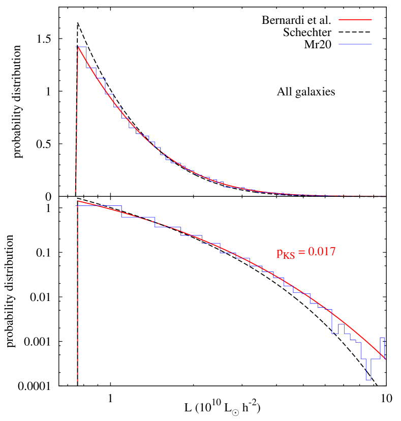
Figure 1: Luminosity distribution of the Mr20 galaxy catalog from Berlind et al. (2006) which contains groups with $N>2$ members (histogram). Solid curve shows equation (6)) with parameters from equation (7). We also display the $p$-value from a KS analysis comparing the data with the solid curve. For comparison, dashed curve, which predicts a slightly fainter distribution than observed, shows the Schechter distribution with parameters from Blanton et al. (2003).

For comparison, the dashed curve shows equation (6) with parameters derived from Blanton et al. (2003) (equation 8). This form predicts somewhat fainter galaxies than are present in the B06 sample. This is not surprising given previous work showing that that the Schechter parametrization is a poor description of the bright-end of the all-galaxy sample, and groups are expected to preferentially host the brightest galaxies. (A KS analysis in this case gives a negligibly small $p$-value.)

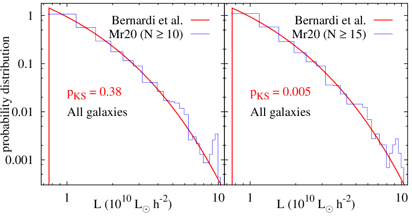
Figure 2: Luminosity distribution of subsamples of the Mr20 galaxy catalog containing groups with $N\geq 10$ and $N\geq 15$ members (histograms). Solid curve in each panel is the same as in Figure 1, and shows $p_{\rm gal}(L)$ (equation 6 using equation 7). This same function provides an accurate description of each subsample. We also display the $p$-values from a KS analysis comparing the data with the solid curve.

As mentioned previously, we do not expect to obtain robust results for groups with $N<10$ and we will henceforth discard these objects. Figure 2 shows the luminosity distributions in two subsamples constructed by restricting to $N\geq 10$ and $N\geq 15$ members. Equation (6) with parameters from equation (7) is an accurate description of each subsample. We show the KS $p$-values from a comparison of each subsample with this distribution. This suggests that these B06 group galaxies are in fact drawn from a universal luminosity distribution which is approximately independent of group richness and halo mass.

It is not a priori obvious that this distribution should have been universal, nor is it obvious that this universal function should have simply been the all-galaxy luminosity function (truncated to only include objects that are brighter than $M_{r}<-19.9$). The latter is worrying, because it might arise as follows. Separating true group members from interlopers on the basis of angular position and redshift space information alone is known to be difficult. Using colors to help identify members of the same group helps significantly, but the B06 algorithm does not use color information. So it is conceivable that the algorithm returns an accurate estimate of the number of members in a group, without actually identifying the members themselves correctly. In this case, it is possible that objects identified in the catalog as group members are effectively random samples of the underlying galaxy distribution – with the choice of link-length parameters having been (too) strongly influenced by theoretical expectations about what the distribution of $N$ should be. If this is indeed why the all-galaxy luminosity function describes the B06 luminosities, then it would invalidate a number of published analyses based on this catalog – particularly those which seek to constrain the phenomenon known as assembly bias. Section 4 describes a novel test of this possibility, which uses mark correlations.

In the remainder of the paper, when discussing the Mr20 catalog, we will show results obtained assuming universality of $p_{\rm gal}(L)$ using equation (6) with parameters from equation (7).

3.2 Central galaxies as statistical extremes

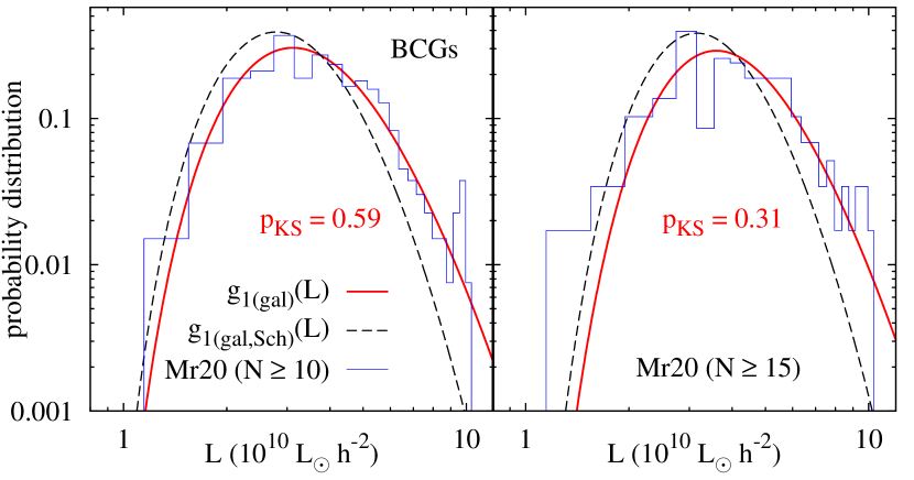
Figure 3: Luminosity distribution of the BCGs in subsamples of the Mr20 catalog with $N\geq 10$ and $N\geq 15$ (histograms). Solid curves show the extreme value statistics for the brightest object in $N$ independent draws from the distribution $p_{\rm gal}(L)$ of equation (6) with parameters from equation (7), averaged over the observed distribution of $N$ in each subsample as in equation (13). We also display the corresponding $p$-values from a KS analysis comparing the data with the solid curves. For comparison, dashed curves show the corresponding predictions using the Blanton et al. parameters from equation (8).

We now ask if the BCG of a group with $N$ members can be described as the brightest of $N$ independent draws from $p_{\rm gal}(L)$. Since the number of groups in the Mr20 catalog with exactly $N$ galaxies where $N\geq 10$ is small, we make this comparison by constructing subsamples restricted to a minimum value of $N$ as in section 3.1 above. In this case, the corresponding theory prediction must be averaged over the allowed values of $N$. We do this by constructing the distribution $p(N)$ directly from the given subsample, and averaging equation (2) over this distribution:

$$g_{1}^{\rm(gal)}(L)=\sum_{{\rm allowed}\ N}g_{1}^{\rm(gal)}(L|N)\,p(N)\,.$$ (13)

Figure 3 shows the results for subsamples of Mr20 containing $N\geq 10$ and $N\geq 15$ members. The solid red curves show the extreme value prediction (13) using equation (6) with parameters from equation (7), together with the respective $p$-values from a KS analysis. We see a remarkable agreement between the predictions and the data. (Of course, $p(N)$ is different for each subsample.) For comparison we also show the predictions when using the Blanton et al. parameters from equation (8). (In this case the KS analysis gives tiny $p$-values $\lesssim 10^{-7}$.)

3.3 Satellite luminosity distribution

We now analyse the satellites in the Mr20 catalog, i.e. the data set obtained by subtracting the BCGs from the full catalog. The results of the previous section allow us to use the satellite luminosity distribution to perform a consistency check. If the full galaxy luminosity distribution $p_{\rm gal}(L)$ is indeed universal, and if the BCGs obey the extreme value statistics of $p_{\rm gal}(L)$, then the satellite luminosity distribution of the subsamples with $N\geq 10$ and $N\geq 15$ must depend on the minimum number of members in a specific way: the predicted distribution is the average of equation (19), weighted by the number of satellites $N-1$, over the observed distribution of $N$. The dotted curves show these predictions; they provide a good description of the data. The associated $p$-values from a KS test are also shown.

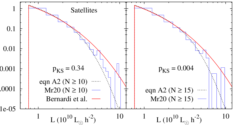
Figure 4: Luminosity distribution of the satellites in subsamples of the Mr20 catalog with $N\geq 10$ and $N\geq 15$ (histograms). Dotted curves show the result of assuming that the satellite distribution is given by subtracting from the full galaxy distribution the associated extreme value distribution, averaged over the observed distribution of $N$ (the average of equation 19, weighted by the number of satellites $N-1$, over $N$). The KS $p$-values associated with the dotted curves are also displayed. Solid curve in each panel is the full galaxy distribution $p_{\rm gal}(L)$ of equation (6) with equation (7).

The solid curves (same in each panel) show $p_{\rm gal}(L)$ from equation (6) with equation (7). The analysis in Appendix A predicts that the satellite distributions at large $N$ should become approximately universal, asymptotically approaching the distribution $p_{\rm gal}(L)$, and we see that this is indeed the case.

3.4 Brightest satellites as second brightest objects

The brightest satellites are, in a sense, more interesting than the BCGs, because there are two statistical contenders for describing their luminosity distribution.

The first is motivated by the fact that BCGs appear to be consistent with extreme value statistics (equation 6 in equation 4). This suggests that the BSGs ought to be well described as the second brightest of $N$ independent draws of the universal galaxy distribution $p_{\rm gal}(L)$ (equation 6 with equation 7 in equation 4). Figure 5 shows that this is indeed the case.

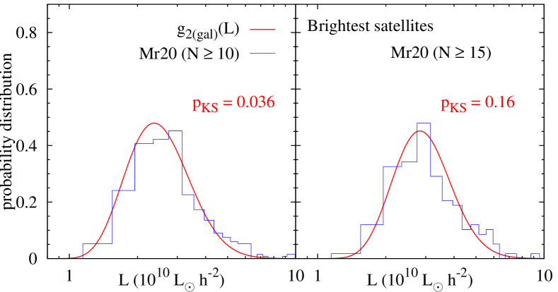
Figure 5: Luminosity distribution of the brightest satellites in subsamples of the Mr20 catalog containing $N\geq 10$ and $N\geq 15$ members (histograms). Solid curves show the order statistics for the second brightest object in $N$ independent draws from the distribution $p_{\rm gal}(L)$ of equation (6) with equation (7), averaged over the observed distribution of $N$, similarly to equation (13) but using the extreme value distribution from equation (4). The corresponding KS $p$-values are also displayed.

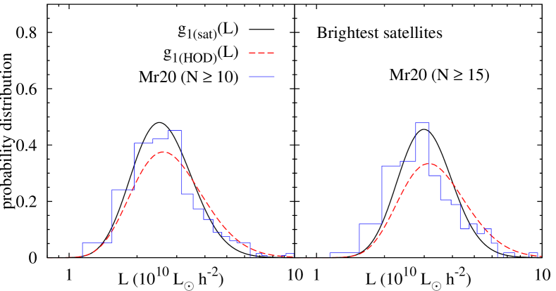
Figure 6: Luminosity distributions of the brightest satellites in two subsamples of the Mr20 catalog: histograms are the same as in Figure 5. Solid black curves show the extreme value statistics for the brightest object in $N_{\rm sat}$ independent draws from the distribution $p_{\rm sat}(L)$. We used extreme value predictions of the corresponding dotted curves of Figure 4 (i.e., $g_{\rm 1sat}(L|N)$ from equation 20, averaged over the observed $N_{\rm sat}$ values). Dashed red curves show the analogous extreme value distributions based on the HOD model of Zehavi et al. (2011) described in Appendix C.

3.5 Brightest satellites as statistical extremes

The alternative model is that BSGs are extremes of some universal satellite distribution, as suggested by the HOD model, and by the measurements which suggest that the overall satellite luminosity function is basically independent of group richness (Skibba et al. 2007; Hansen et al. 2009). Figure 6 shows this comparison for two choices of the universal distribution $p_{\rm sat}(L)$. More precisely, we compare the brightest satellite distributions for the two subsamples (the histograms are the same as in Figure 5), with the extreme value distribution appropriate for the brightest of $N_{\rm sat}$ independent draws of an assumed universal satellite distribution $p_{\rm sat}(L)$, averaged over the observed distribution of $N_{\rm sat}$ values (solid and dashed curves, see below). The resulting extreme value distribution is identical in form to equations (13) and (2), with $N\to N_{\rm sat}$ and $p_{\rm gal}(L)\to p_{\rm sat}(L)$. These predictions depend on $p_{\rm sat}(L)$.

The solid curves show the result of using our analytic calculation of $p_{\rm sat}(L)$ (dotted curves in Figure 4) to provide a calculation of $g_{\rm 1sat}(L|N)$ (from equation 20) which we then average over the observed distribution of $N_{\rm sat}$. The solid curves provide a good description of the measurements, with KS $p$-values comparable to those in Figure 5; this is not surprising since we are at large $N$, where we know that $g_{\rm 1sat}\to g_{\rm 2gal}$ (see discussion at the end of Appendix A). Unfortunately then, this large $N$ dataset is not suitable for distinguishing between these two predictions.

The dashed curves show the result of using the HOD result equation (29). We see that this tends to always predict brighter distributions than the ones observed (the corresponding KS $p$-values are $\sim 10^{-5}$). However, since the HOD prediction relies on parameter values derived from statistical fits (Zehavi et al. 2011), we would caution against taking these results at face value. A more complete treatment would involve accounting for parameter errors in the HOD fit, but this is beyond the scope of this work.

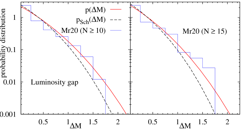
Figure 7: Distribution of the luminosity gap $\Delta M$ for subsamples of the Mr20 catalog with $N\geq 10$ and $N\geq 15$ (histograms). The solid curves are the corresponding predictions of extreme value statistics equation (17), averaged over the corresponding observed distributions of $N$ and using $p_{\rm gal}(L)$ from equation (6) with equation (7). For comparison, we also show the predictions based on parameters from equation (8).

3.6 The luminosity gap

If both the BCG and BSG luminosity functions are given by Order Statistics, then the joint distribution of their magnitudes $p(M_{1},M_{2}|N)$ (with $M_{j}$ being the $j^{\rm th}$ brightest) is

$$p(M_{1},M_{2}|N) =N(N-1)p_{\rm gal}(M_{1})$$

$$\phantom{N}\times p_{\rm gal}(M_{2})P_{\rm gal}(>M_{2})^{N-2}\Theta(M_{2}-M_{1})\,,$$ (14)

with $\Theta(x)$ the Heaviside distribution, and we have used the same notation $p_{\rm gal}$ as before to denote the universal galaxy luminosity distribution, with $p_{\rm gal}(m)=L(m)p_{\rm gal}(L(m))\ln(10)/2.5$. This allows us to derive the distribution of the luminosity gap, defined as the difference in magnitudes $\Delta M\equiv M_{2}-M_{1}$ of the second brightest and brightest objects. Before considering this distribution, we note that another interesting distribution is that of the second brightest $M_{2}$, for a fixed value of $M_{1}$. This is given by

$$p(M_{2}|M_{1},N) =\frac{p(M_{1},M_{2}|N)}{p(M_{1}|N)}$$

$$=(N-1)p_{\rm gal}(M_{2})\frac{P_{\rm gal}(>M_{2})^{N-2}}{P_{\rm gal}(>M_{1})^{N-1}}\Theta(M_{2}-M_{1})\,.$$ (15)

As $M_{1}$ is made more negative, i.e. as the BCG is made more luminous, $P_{\rm gal}(>M_{1})\to 1$, and this distribution simply asymptotes to that of the brightest of $N-1$ draws from the universal galaxy distribution, independent of $M_{1}$. In other words, the typical gap $\Delta M$ increases as the BCG is made more luminous, illustrating what is known as the Bautz & Morgan (1970) effect. We can therefore understand the latter as a straightforward consequence of order statistics.

The distribution of the luminosity gap $\Delta M$ for fixed $N$ is predicted to be

$$p(\Delta M|N) =N(N-1)\int dm\,p_{\rm gal}(m)$$

$$\phantom{N(-1)}\times P_{\rm gal}(>m)^{N-2}p_{\rm gal}(m-\Delta M)\,.$$ (16)

As with the earlier distributions, we can define averages of the fixed-$N$ gap distribution over subsamples, as

$$p(\Delta M)=\sum_{{\rm allowed}N}p(\Delta M|N)p(N)\,.$$ (17)

Figure 7 compares the averaged prediction in equation (17) with the subsamples of Mr20 having $N\geq 10$ and $N\geq 15$. We see a good visual agreement between the data and the prediction based on equation (6) with equation (7) (solid curves), except at small $\Delta M$, where the data show a number of groups with $\Delta M$ precisely equal to zero. We have checked that all these systems correspond to fiber collided BCGs, and the algorithm of B06 then assigns the brightest satellite both the redshift and the absolute magnitude of the BCG. The KS $p$-values comparing the solid curves to the full data (i.e., including the cases with $\Delta M=0$) are negligibly small. However, comparing the same curves after subtracting the spike from the data leads to large $p$-values ($>0.1$). In either case (with or without the spike), using equation (6) with equation (7) provides a better description of the large $\Delta M$ tail than using equation (8).

4 Mark correlations as a novel test of order statistics

The previous section showed that the distribution of group-galaxy luminosities was very like that of all galaxies (whether or not they are in groups). This raised the question of whether or not the group catalog has correctly separated group members from the field. We will use mark correlations to address this and related questions.

The mark correlation $WW(r)/DD(r)$ is a statistic associated with pairs of objects separated by $r$; $DD(r)$ is the number of pairs of separation $r$, and $WW(r)$ is the result of weighting each galaxy $i$ by some weight $W_{i}/\bar{W}$, (where $\bar{W}$ is the average weight of the sample) when performing the pair count. In what follows, we will use the luminosity as a weight. If there is no correlation between a galaxy’s luminosity and its position then $WW/DD$ should be unity; departures from unity indicate that the luminosities and positions are correlated.

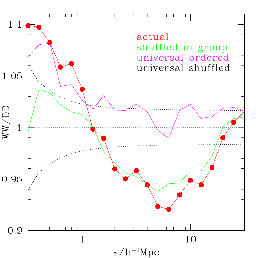
Figure 8: Luminosity mark correlation in the Mr20 catalog, restricted to galaxies which reside in groups with more than 10 members (red symbols). The fact that this signal is different from unity on small scales ($<1h^{-1}$Mpc) indicates a significant correlation between luminosity and location within the group. The fact that it is also different from unity on larger scales shows that the luminosity function cannot be universal. This is more clearly demonstrated by the ‘universal ordered’ (magenta) and ‘shuffled in group’ (green) curves which separate these two effects (see text). The dotted curves (‘universal shuffled’) are a rough measure of the statistical significance of the difference from unity.

We begin with the objects in the Mr20 group catalog. If the group-identification process ended up assigning random galaxies to groups, then the catalog which results from scrambling the list of luminosities among all the members of the original catalog should be stastically the same as the original one. Therefore, we measure the luminosity mark correlation $WW/DD$ in this scrambled catalog. We find that $WW/DD\sim 1$ as it should. Repeating this scrambling procedure a few times and averaging the results gives some indication of the range of values around unity that one might expect given the observed set of $L$ and positions, if the luminosities and positions are indeed uncorrelated. The dotted curves in Figure 8 show this range, which we will use as a rough measure of the significance of a detection of a correlation between luminosity and position.

Next, we scramble the luminosities as before – thus erasing any possible correlations – but then, within each group, we reassign the luminosities among the objects in the group so that they have the same rank-ordering as in the actual dataset. The resulting measurement of $WW/DD$ shows the expected signal if the luminosity distribution were universal (i.e. the same for all groups), but the distribution within a group depends on location within the group (e.g., if the central galaxy is the brightest). The figure shows the result of averaging $WW/DD$ over many such ‘universal ordered’ rescramblings (magenta curve). There is a clear tendency for $WW/DD>1$ at $r\leq 1h^{-1}$Mpc, indicating a stastically significant correlation between galaxy luminosity and group-centric position. Notice, however, that $WW/DD$ declines to $\sim 1$ on larger scales; this is a consequence of the fact that the typical group size is of order $r\leq 1h^{-1}$Mpc, and we have erased all correlations on larger scales. (In the Halo Model description of mark correlations (Sheth 2005), the two-halo term for this case is unity.)

Finally, the filled red symbols show $WW/DD$ in the original (unscrambled) group catalog. On small scales, the signal is similar to that in the ‘universal ordered’ groups, but it clearly differs from unity even on larger scales. The fact that $WW/DD\neq 1$ on $>1h^{-1}$Mpc scales suggests that the luminosity function itself is not universal. To separate out the effects of the group-centric trends from possible group-group trends, we have performed a final scrambling. We keep the list of luminosities within a group the same, but, within each group, we scramble the luminosities amongst the group members. In this way, we remove that part of the signal from $WW/DD$ which is due to the correlation with group-centric position. Notice that now $WW/DD$ (‘shuffled in group’, green curve) is like the original on large scales, but it does not increase as much on smaller ($<1h^{-1}$Mpc) scales.

Thus, our mark correlation analysis has shown that i) group-centric position matters; and ii) even once this has been accounted for, the luminosity function is not universal for all groups. The first point derives from the fact that the ‘universal ordered’ signal is not unity on small scales, and it is very similar to the original one, and the ‘shuffled in group’ signal differs from the original unscrambled one at these small scales. This strongly suggests that the brightest cluster galaxy does indeed lie closer to (if not at) the group center. And the fact that, on larger scales, the actual signal differs so significantly from the ‘universal ordered’ one (i.e. from unity) indicates that the luminosity function cannot be the same for all groups. This was not at all obvious from the (more traditional) analysis of the group and BCG luminosity functions in the previous section.

5 Conclusions

Brightest cluster galaxies are interesting for several reasons, the simplest being that they are the brightest and therefore most easily observable of galaxies. As mentioned in the Introduction, it is also becoming increasingly certain that they are physically distinct in several other ways, e.g. in their morphology, velocity dispersions, etc., from the other galaxies (the satellites) which reside in groups and clusters. We argued that, from the point of view of Halo Model analyses, it is interesting to ask whether the luminosities of the BCGs retain any signature of their special nature. Our analysis shows that, at the level of one-point distributions, the answer appears to be ‘no’: BCG luminosities (insofar as they are accurately represented in the Mr20 catalog that we analysed) are consistent with being the statistical extremes of a universal luminosity function, which is well-described by equation (6).

We also analysed the luminosity functions of the satellites in the Mr20 catalog. The behaviour of these distributions for different values of group richness (i.e. number of members) $N$ is especially interesting, since it potentially allows us to distinguish between two seemingly reasonable but incompatible predictions of Halo Model analyses. On the one hand, since the BCG luminosities are simply statistical extremes of a universal galaxy luminosity distribution, it is reasonable to expect that (a) the satellite luminosity function is just that given by subtracting the BCGs from the universal one (equation 19), and (b) the brightest satellite (BSG) luminosities are simply the second brightest of $N$ draws of the universal galaxy distribution. On the other hand, the HOD model predicts that (c) the satellite function is itself approximately universal, and (d) the BSGs are statistical extremes of this function. We showed that these two sets of predictions are inequivalent in general. In the present case, however, the large values of $N$ that we consider prevent us from distinguishing between these two predictions, each of which provides an acceptable description of the data.

Additionally, we performed other tests to check the consistency of our results. We showed that the statistics of the luminosity gap (the difference in absolute magnitudes of the BSG and BCG) in the Mr20 catalog are consistent with the predictions of order statistics (equation 16). In Appendix B we argued that statistical tests for the mean BCG luminosity based on fixed $N$ are to be preferred over those based on, say, fixed total group luminosity $L_{\rm tot}$, showing how the latter may lead to biased conclusions. We also emphasized that, in order to perform unbiased tests, it is crucial to use accurate descriptions of the bright tail of the galaxy luminosity function.

However, we showed that, at the level of two-point statistics, the BCG and BSG luminosity distributions are inconsistent with their having being drawn from a universal luminosity function (i.e., one that is the same for all groups). We argued that because the luminosity mark correlation function differs significantly from unity on large scales (Figure 8) the luminosity function of groups must depend on group properties (e.g. mass). This was not at all obvious from the (more traditional) one-point analysis of the group and BCG luminosity functions themselves.

In work in progress, we show that the extreme values assumption together with a universal luminosity distribution $p_{\rm gal}(L)$ predicts a halo mass dependent BCG luminosity function $g_{1}(L|m)=\sum_{N}p(N|m)g_{1}(L|N)$ if the distribution of $N$ depends on mass $m$. This would have immediate consequences for implementations of the Halo Model such as the Halo Occupation Distribution (HOD, Zehavi et al. 2005), since such analyses would considerably simplify upon imposing the extreme value restriction on the BCG luminosities. However, we have already seen that the assumption of universality is inconsistent with the observed mark correlation signal on large scales. One might then wonder if the correct solution is to replace $p_{\rm gal}(L)\to p_{\rm gal}(L|m)$. In this case, the BCG luminosity function averaged over $N$ is mass dependent because both $p_{\rm gal}$ (and hence $g_{1}(L|N,m)$) and $p(N|m)$ depend on $m$. In this case it is no longer obvious that the extreme values hypothesis should be tested at fixed $N$ as we argued earlier. Formulating the problem cleanly in this case is work in progress.

Additionally, as discussed in the Introduction, this behaviour of the BCG luminosities, in particular, the fact that their luminosity functions are narrower than those of all galaxies, potentially allows BCGs to be used for consistency checks of standard candle constraints on the luminosity-distance relation. As a final remark, we note that, while BCGs have brighter and narrower luminosity distributions than randomly picked galaxies, the distributions of the BSG luminosities are even narrower than those of the BCGs. From the point of view of using them as standard candles, an interesting trade-off then arises: while it is the BCG which is most easily observed out to large distances, the BSG is a more standard candle. It will be interesting to see to what extent these ideas can be implemented in upcoming cluster surveys.

Appendix A Prediction for the satellite luminosity distribution from extreme value statistics

If the luminosity distribution of galaxies $p_{\rm gal}(L)$ is universal, and if the BCGs in groups containing $N$ members are described as the brightest objects of $N$ independent draws from this distribution, then the distribution of the satellites in such groups must have a specific dependence on $N$, as we show below.

Consider a sample of $\mathcal{N}_{{\rm g}|N}^{>L_{\rm min}}$ galaxies brighter than $L_{\rm min}$, residing in $\mathcal{N}_{{\rm h}|N}^{>L_{\rm min}}$ groups (halos) which contain exactly $N$ members each, so that $\mathcal{N}_{{\rm g}|N}^{>L_{\rm min}}=N\mathcal{N}_{{\rm h}|N}^{>L_{\rm min}}$. Since $p_{\rm gal}(L)$ is universal, the number of these galaxies brighter than $L$, is $\mathcal{N}_{{\rm g}|N}^{>L}=\mathcal{N}_{{\rm g}|N}^{>L_{\rm min}}P_{\rm gal}(>L)$. Similarly, the number of BCGs brighter than $L$ is $\mathcal{N}_{{\rm BCG}|N}^{>L}=\mathcal{N}_{{\rm h}|N}^{>L_{\rm min}}g_{1}(>L|N)$, where $g_{1}(>L|N)=1-P_{\rm gal}(<L)^{N}$ follows from equation (1).

The satellites are obtained by subtracting the BCGs from the full sample, and the number of satellites brighter than $L$ is therefore $\mathcal{N}_{{\rm sat}|N}^{>L}=\mathcal{N}_{{\rm g}|N}^{>L}-\mathcal{N}_{{\rm BCG}|N}^{>L}$, which tells us that $P_{\rm sat}(>L|N)$ is

$$P_{\rm sat}(>L|N) =\frac{\mathcal{N}_{{\rm sat}|N}^{>L}}{\mathcal{N}_{{\rm sat}|N}^{>L_{\rm min}}}=\frac{\mathcal{N}_{{\rm g}|N}^{>L}-\mathcal{N}_{{\rm BCG}|N}^{>L}}{\mathcal{N}_{{\rm g}|N}^{>L_{\rm min}}-\mathcal{N}_{{\rm h}|N}^{>L_{\rm min}}}$$

$$=\frac{1}{N-1}\left(NP_{\rm gal}(>L)-g_{1}(>L|N)\right)$$

$$=1-\frac{NP_{\rm gal}(<L)-P_{\rm gal}(<L)^{N}}{N-1}$$

$$=P_{\rm gal}(>L)-\frac{P_{\rm gal}(<L)-P_{\rm gal}(<L)^{N}}{N-1}\,,$$ (18)

which gives a satellite luminosity distribution

$$p_{\rm sat}(L|N)=\frac{1}{(1-1/N)}p_{\rm gal}(L)\left(1-P_{\rm gal}(<L)^{N-1}\right)\,.$$ (19)

Notice that for large enough richness values $N$, $1-1/N\to 1$ and $P_{\rm gal}(<L)^{N-1}\to 0$, for all interesting values of $L$, and hence $p_{\rm sat}(L|N\gg 1)\to p_{\rm gal}(L)$. Figure 4 shows that averaging this distribution over the observed distribution of $N$ provides a good description of the distribution of satellite luminosities in the B06 group catalog, especially at large $N$.

The extreme value statistics associated with this distribution yields

$$g_{\rm 1sat}(<L|N)=\left(\frac{NP_{\rm gal}(<L)-P_{\rm gal}(<L)^{N}}{N-1}\right)^{N-1},$$ (20)

which is clearly different from $g_{2}(<L|N)$ in the main text. Although they are different for general $N$, it is easy to show that

$$g_{\rm 1sat}(<L|N)\to g_{2}(<L|N)\qquad{\rm as}\quad N\gg 1;$$ (21)

i.e., the distribution of the largest of $N-1$ picks from the satellite distribution does indeed tend to that of the second largest of $N$ picks from the full distribution. We check this explicitly in Figure 6 of the main text.

Appendix B A shuffling-based test of extreme value statistics

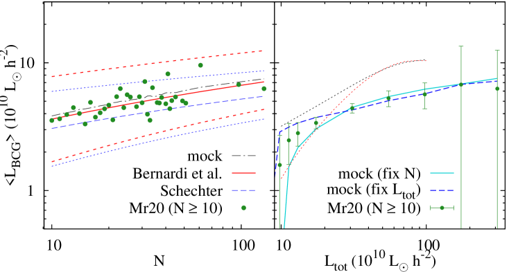
Figure 9: Mean value of $L_{\rm BCG}$ as a function of group size $N$ (left) and $L_{\rm tot}$ (right) in the B06 Mr20 catalog (symbols). (Left panel): Dotted-dashed line shows the mean relation between $L_{\rm BCG}$ and $N$ in 500 mock catalogs obtained by scrambling the observed list of galaxy luminosities and constructing groups such that the observed distribution of $N$ values is reproduced (see text). Solid red curve shows the mean prediction of extreme value theory based on equation (6) with equation (7), while red short-dashed curves indicate the corresponding region enclosing 95% of probability for each $N$. The data, mocks and theory predictions are in excellent agreement. Blue long-dashed and corresponding dotted curves show the mean and 95% region of extreme value theory based on the Schechter form of Blanton et al. (2003) equation (8), and emphasize that using an inaccurate description of the bright tail of the galaxy luminosity function can lead to erroneous conclusions regarding, e.g., the statistical significance of outliers. (Right panel:) Solid line shows the mean relation between $L_{\rm BCG}$ and $L_{\rm tot}$ in the same mocks which gave the dotted-dashed curve of the left panel. The data agree very well with these mocks, although they seem to lie systematically slightly higher than the curve at small $L_{\rm tot}$. Dashed curve shows the same mean relation, but in mocks generated by fixing an observed $L_{\rm tot}$ value and randomly sampling the observed galaxy luminosity list until the total luminosity exceeds this $L_{\rm tot}$ (see text for more details). This procedure, in general, does not reproduce the observed distribution of $N$, and leads to biased conclusions regarding the mean relation. The dotted curves explicitly demonstrate this bias for the exponential luminosity distribution $P(>L)={\rm e}^{-(L-L_{\rm min})/L_{\ast}}$ by plotting $\langle\,L_{\rm BCG}|L_{\rm tot}\,\rangle$ for two choices of the distribution of richness $p(N)$ (see text).

In the main text, we argued that equation (6), with parameters from Bernardi et al. (2010) provided a good fit to the distribution of luminosities in the B06 group catalog. Here, we provide additional tests of this assumption. We also make two points: First, when one is interested in deriving constraints from the extreme tails of a distribution, then it is important to have an accurate description of the tails. Second, when testing extreme value or, more generally, order statistics, the test is best done keeping $N$ fixed.

A simple test of whether or not BCG luminosities are unusual compared to those of the other galaxies in the group is to make a mock catalog by scrambling the list of galaxy luminosities among the different groups. The BCG luminosity distribution in the mock catalog represents the expected distribution if BCGs were not otherwise special, and comparison with the BCGs in the original dataset indicates if they are indeed special. In practice, we generate 500 realizations of the scrambled mock catalog, so as to produce a less noisy estimate of the expected extreme value distribution.

The B06 groups are characterized by two numbers: the total number of galaxies, $N$, and the total luminosity of the group $L_{\rm tot}$ (simply the sum of the luminosities of $N$ group members). When generating the mock catalog, we must decide whether to keep $N$ or $L_{\rm tot}$ fixed. Order statistics are clearly a function of $N$, so $N$ is the natural variable. However, one might be concerned that the luminosity of the BCG depends on ‘hidden’ variables, such as halo mass. If so, if one believes $L_{\rm tot}$ is a better indicator of this hidden variable, then one might wish to make mocks by holding it, rather than $N$, fixed. We will show results of doing both, but note that the results in the main text strongly suggest that the test at fixed $N$ is the prefered one.

To generate a mock catalog, we first randomly scramble the observed list of galaxy luminosities (which we take from groups with $N\geq 10$). We then run over the observed values of $N$, sequentially picking $N$ luminosities from the scrambled list for each $N$, and store both the sum and the largest of these $N$ picks. We then move on to the next value of $N$. This procedure, by construction, reproduces the observed distribution of $N$ values.

The dotted-dashed curve in the left hand panel of Figure 9 shows the resulting correlation between $N$ and $L_{\rm BCG}$ in the mocks. This curve represents the extreme value prediction for the $L_{\rm BCG}$, if BCGs are just the extremes of the group-galaxy luminosity function. The symbols show the actual correlation in the Mr20 catalog (wherever possible, we average over the BCG luminosities at fixed $N$). We have deliberately chosen to show the log of $L_{\rm BCG}$ because the extreme value distribution has a long tail to large $L$ – showing the log brings the visual impression of the scatter around the mean value closer to the correct one.

The solid curve shows the associated prediction for this correlation if we insert equation (6) in equation (2). It lies very close to the dotted-dashed curve. This is consistent with one of the points made in the main text: that the all-galaxy luminosity function, equation (6) with equation (7), provides an excellent description of the Mr20 group-galaxy luminosities. (The fact that it is systematically beneath the dot-dashed curve is consistent with the fact that the galaxies in this sample are slightly brighter than predicted by $p_{\rm gal}(L)$.) The short dashed curves on either side of it indicate the region which contains 95% of the probability (at each $N$), also calculated from equation (2). We note that none of the observed groups lie outside this region.

The other dashed curve, and associated 95% regions, shows the extreme-values prediction if we use the Schechter function of Blanton et al. (2003), equation (8), instead. This curve falls below that of our mock catalogs. Since a number of the Mr20 points lie outside its 95% band, had one used this curve, rather than performing the full shuffling procedure, one might have concluded that the BCGs in the Mr20 catalog are inconsistent with the extreme values hypothesis. However, this conclusion is unwarranted, because the Schechter function does not describe the bright-end of the group-galaxy distribution very well (see Figure 1). Thus, the exercise above illustrates the importance of using accurate measures of the tail, if one intends to use the tail to draw important conclusions.

The panel on the right shows the correlation between $L_{\rm BCG}$ and $L_{\rm tot}$ in the Mr20 catalog (symbols) and in the mock catalogs which were used to produce the panel on the left (solid curve). The agreement is very good, at least at large $L_{\rm tot}$, again indicating that BCG luminosities are consistent with just being statistical extremes. We have also checked that the mean $L_{\rm tot}$ at fixed $N$ is close to being proportional to $N$ for this catalog, with the best fit power law relation being $L_{\rm tot}=1.66\times 10^{10}L_{\odot}h^{-2}N^{0.96}$.

The dashed curve, which lies above the measurements at small $L_{\rm tot}$ but close to the solid curve at larger $L_{\rm tot}$ was obtained by generating mock catalogs following a slightly different procedure – one that is essentially the same as that recently used by Lin et al. (2010) in their analysis of BCG luminosities in another group catalog. In this case, for each observed $L_{\rm tot}$, we continue to draw luminosities from the group galaxy distribution until the sum of these luminosities first exceeds $L_{\rm tot}$. We then compare this value and the one preceding it to the observed value, and assign the closer of the two to the mock group. We also determine the luminosity of the mock BCG from the list of luminosities which contribute to the group’s luminosity, before moving on to the next value of $L_{\rm tot}$. To obtain smoother results, we run over the observed distribution of $L_{\rm tot}$ values 500 times.

In this case, there is no guarantee that the mock catalog which results has the correct distribution of $N$. Since extreme value statistics are explicitly a function of the number of draws $N$ (e.g. equations 2 and 4), it seems unlikely that this procedure can yield a fair test of these statistics. Indeed, the difference between the dashed and solid curves in this panel is a measure of the bias in this particular test, since the solid line is associated with mock catalogs that, as shown in the panel on the left, are in excellent agreement with the expected extreme value distribution.

This is easier to appreciate with a simpler example. When the universal function $p(L)$ is an exponential, $P(>L)={\rm e}^{-(L-L_{\rm min})/L_{\ast}}$, then the mean BCG luminosity at fixed $L_{\rm tot}$ and $N$ takes the form

$$\langle\,L_{\rm BCG}|L_{\rm tot},N\,\rangle=L_{\rm min}+\frac{H_{N}}{N}(L_{\rm tot}-NL_{\rm min})$$ (22)

(defined for $L_{\rm tot}\geq NL_{\rm min}$), where $H_{N}=\sum_{r=1}^{N}(1/r)$ is a harmonic number. The mean BCG luminosity is then $\langle\,L_{\rm BCG}|L_{\rm tot}\,\rangle=\sum_{N}\langle\,L_{\rm BCG}|L_{\rm tot},N\,\rangle p(N|L_{\rm tot})$. The distribution $p(N|L_{\rm tot})$ is constructed as $p(N|L_{\rm tot})=p(L_{\rm tot}|N)p(N)/\sum_{N^{\prime}}p(L_{\rm tot}|N^{\prime})p(N^{\prime})$, where

$$L_{\ast}p(L_{\rm tot}|N)=\frac{{\rm e}^{(L_{\rm tot}-NL_{\rm min})/L_{\ast}}}{(N-1)!}\left(\frac{L_{\rm tot}-NL_{\rm min}}{L_{\ast}}\right)^{N-1}\,,$$

which is also defined for $L_{\rm tot}-NL_{\rm min}>0$ and is zero otherwise.

One therefore needs to choose a “prior” distribution $p(N)$, and the dotted curves in right panel show $\langle\,L_{\rm BCG}|L_{\rm tot}\,\rangle$ for the exponential luminosity distribution when $p(N)$ is the one observed in the data (lower, red) and in the mocks described above which kept $L_{\rm tot}$ fixed (upper, black). We see that the difference between the curves has the same sense as that for the mocks based on the actual luminosity distribution. This explicitly demonstrates the bias introduced by using the wrong distribution of $N$.

We conclude that the BCG luminosities in the Mr20 group catalog are consistent with being the statistical extremes of the group-galaxy luminosity function – the latter being very well described by the all-galaxy luminosity function.

Appendix C The HOD model of Zehavi et al. (2011)

The HOD implementation of Zehavi et al. (2011) parametrizes the mean number of galaxies $\langle\,N|>L,m\,\rangle$ brighter than some threshold $L$ in a halo of mass $m$ using

$$\langle\,N|>L,m\,\rangle=f_{\rm cen}(>L,m)\left(1+\bar{N}_{\rm sat}(>L,m)\right)\,,$$ (23)

where

$$f_{\rm cen}(>L,m) =\frac{1}{2}\left(1+{\rm erf}\left(\frac{\log m-\log M_{\rm min}(L)}{\sigma_{\log M}(L)}\right)\right)\,,$$ (24)

$$\bar{N}_{\rm sat}(>L,m) =\left(\frac{m-M_{0}(L)}{M_{1}^{\prime}(L)}\right)^{\alpha(L)}\,.$$ (25)

The function $f_{\rm cen}(>L,m)$ is interpreted as the number of centrals, and the product of $f_{\rm cen}(>L,m)$ and $\bar{N}_{\rm sat}(>L,m)$ as the mean number of satellites in the $m$-halo. It is natural to interpret these functions in terms of conditional probabilities, with $f_{\rm cen}(>L,m)$ being the fraction of $m$-halos that host a central galaxy (note that it varies between 0 and 1 by definition) and $\bar{N}_{\rm sat}(>L,m)$ being the mean number of satellites in halos that host a central. The distribution of the number of satellites brighter than $L$ in an $m$-halo which hosts a central is assumed to be Poisson with mean $\bar{N}_{\rm sat}(>L,m)$.

The values of the parameters $M_{\rm min},\sigma_{\log M},M_{0},M_{1}^{\prime}$ and $\alpha$ at various thresholds are then fit by comparing a Halo Model calculation of the projected $2$-point correlation function to measurements of luminosity dependent clustering in SDSS data. The results are in Table 3 of Zehavi et al. (2011), of which we use information for the 5 threshold values brighter than $-19.9$. The HOD prediction for the satellite luminosity distribution is

$$P_{\rm sat}(>L|m,L_{\rm min})=\frac{\bar{N}_{\rm sat}(>L,m)}{\bar{N}_{\rm sat}(>L_{\rm min},m)}\,.$$ (26)

Since this depends on mass, obtaining predictions for the distribution at fixed $N_{\rm sat}$ requires an average over the mass. Following Skibba et al. (2007) we define the number density of groups with $N_{\rm sat}$ satellites

$$n_{\rm grp}(N_{\rm sat}|L_{\rm min})=\int dm\frac{dn}{dm}f_{\rm cen}(>L_{\rm min},m)p(N_{\rm sat}|m,L_{\rm min})\,,$$ (27)

where $dn/dm$ is the halo mass function and $p(N_{\rm sat}|m,L_{\rm min})$ is a Poisson distribution with mean $\bar{N}_{\rm sat}(>L_{\rm min},m)$. For brevity we drop the reference to $L_{\rm min}$ in what follows.

The satellite luminosity distribution at fixed $N_{\rm sat}$ is then given by

$$P_{\rm sat}(>L|N_{\rm sat}) =\int dm\frac{dn}{dm}\frac{f_{\rm cen}(>L_{\rm min},m)}{n_{\rm grp}(N_{\rm sat})}$$

$$\phantom{dmdn/dm}\times p(N_{\rm sat}|m)P_{\rm sat}(>L|m)\,.$$ (28)

This function is then used to compute an extreme value distribution $g_{1\rm sat}(L|N_{\rm sat})$, which is identical in form to equation (2), with $N\to N_{\rm sat}$ and $p_{\rm gal}(L)\to p_{\rm sat}(L|N_{\rm sat})=-\partial P_{\rm sat}(>L|N_{\rm sat})/\partial L$. To be consistent, the prediction for $N_{\rm sat}\geq N_{\rm min}$ must be averaged using the distribution $p(N_{\rm sat})=n_{\rm grp}(N_{\rm sat})/\bar{n}_{\rm grp}$ where $\bar{n}_{\rm grp}=\int dmdn/dmf_{\rm cen}(>L_{\rm min},m)$. In other words,

$$g_{1\rm sat}(L)=\frac{\sum_{N_{\rm sat}\geq N_{\rm min}}g_{1\rm sat}(L|N_{\rm sat})n_{\rm grp}(N_{\rm sat})}{\sum_{N_{\rm sat}\geq N_{\rm min}}n_{\rm grp}(N_{\rm sat})}\,.$$ (29)

Note that computing $g_{1\rm sat}(L|N_{\rm sat})$ requires taking a derivative of $P_{\rm sat}(>L|N_{\rm sat})$. To ensure smooth results, in practice we first fit simple monotonic forms to the values of the various HOD parameters in Table 3 of Zehavi et al. For the mass function we use the analytical approximation of Sheth & Tormen (1999). We have checked that the luminosity dependent clustering predicted by our smooth fits to the Zehavi et al. values is close to the measurements in their Figure 10 and Table 8. We then use $L_{\rm min}=0.747\times 10^{10}L_{\odot}h^{-2}$ and $N_{\rm min}=10$, $15$ to make our predictions. These are shown as the dashed red curves in Figure 6.

References

- [1] Bautz L. P., Morgan W. W., 1970, ApJ, 162, L149
- [2] Berlind A. A., et al., 2006, ApJS, 167,1
- [3] Bernardi M., et al., 2010, MNRAS, 404, 2087
- [4] Bernardi M., Roche N., Shankar F., Sheth R. K., MNRAS, 2011, L6
- [5] Bhavsar S. P., Barrow J. D., 1985, MNRAS, 213, 857
- [6] Blanton M. R., et al., 2003, ApJ, 592, 819
- [7] Cooray A., Sheth R. K., 2002, Phys. Rept., 372, 1
- [8] De Lucia G., Blaizot J., 2007, MNRAS, 375, 2
- [9] Dobos L., Csabai I., 2011, MNRAS, 414, 1862
- [10] Hansen S. M., Sheldon E. S., Wechsler R. H., Koester B. P., 2009, ApJ, 699, 1333
- [11] Hubble E., 1936, ApJ, 84, 270
- [12] Lin Y.-T., Ostriker J. P., Miller C. J., 2010, ApJ, 715, 1486
- [13] Loh Y.-S., Strauss M. A., 2006, MNRAS, 366, 373
- [14] Milosavljević M., Miller C. J., Furlanetto S. R., Cooray A, 2006, ApJ, 637, L9
- [15] Sandage A., Kristian J., Westphal J. A., 1976, ApJ, 205, 688
- [16] Schechter P. L., Peebles P. J. E., 1976, ApJ, 209, 670
- [17] Scott E. L., 1957, AJ, 62, 248
- [18] Sheth R. K., Tormen G., 1999, MNRAS, 308, 119
- [19] Sheth R. K., 2005, MNRAS, 364, 796
- [20] Skibba R. A., Sheth R. K., Martino M. C., 2007, MNRAS, 382, 1940
- [21] Tremaine S. D., Richstone D. O., 1977, ApJ, 212, 311
- [22] Yang X., Mo H. J., van den Bosch F. C., 2008, MNRAS, ApJ, 676, 248
- [23] Zehavi I., et al., 2005, ApJ, 630, 1
- [24] Zehavi I., et al., 2011, ApJ, 736, 59