Fourier Transform Scanning Tunneling Spectroscopy: the possibility to obtain constant energy maps and band dispersion using a local measurement

Abstract

We present here an overview of the Fourier Transform Scanning Tunneling spectroscopy technique (FT-STS). This technique allows one to probe the electronic properties of a two-dimensional system by analyzing the standing waves formed in the vicinity of defects. We review both the experimental and theoretical aspects of this approach, basing our analysis on some of our previous results, as well as on other results described in the literature. We explain how the topology of the constant energy maps can be deduced from the FT of dI/dV map images which exhibit standing waves patterns. We show that not only the position of the features observed in the FT maps, but also their shape can be explained using different theoretical models of different levels of approximation. Thus, starting with the classical and well known expression of the Lindhard susceptibility which describes the screening of electron in a free electron gas, we show that from the momentum dependence of the susceptibility we can deduce the topology of the constant energy maps in a joint density of states approximation (JDOS). We describe how some of the specific features predicted by the JDOS are (or are not) observed experimentally in the FT maps. The role of the phase factors which are neglected in the rough JDOS approximation is described using the stationary phase conditions. We present also the technique of the T-matrix approximation, which takes into account accurately these phase factors. This technique has been successfully applied to normal metals, as well as to systems with more complicated constant energy contours. We present results recently obtained on graphene systems which demonstrate the power of this technique, and the usefulness of local measurements for determining the band structure, the map of the Fermi energy and the constant-energy maps.

I Introduction

One of the most remarkable feats achieved with an STM, beside the possibility to visualize material surfaces with atomic resolution, was the possibility to image the standing waves associated to the interference of quasi-free electron wavefunctions. This has been achieved for the first time on a copper surface, for electrons confined in a circular resonator created with iron ad-atoms, structure well known as a “quantum coral” Crommie93 ; Eigler94 ; Heller94 ; Manoharan2000 . This observation has provided direct evidence that electrons are associated to waves, thus demonstrating the wave-particle duality which is one of the fundamental concepts of quantum mechanics.

The “standing waves” arising in the presence of surface inhomogeneities are also known as Friedel oscillations friedel58 , where the term of Friedel oscillations has been first introduced to describe the asymptotic dependence of the perturbed density of states of a free electron gas in the presence of disorder. Their observation allows the illustration of some very important concepts of condensed matter physics. Thus, the analysis of Friedel oscillations provides a direct observation of screening and of electron-electron interaction. Moreover, these oscillations lie at the foundation of the description of the indirect coupling between magnetic moments via the conduction electrons in a metal with the famous Ruderman-Kittel-Kasuya-Yosida (RKKY) interaction potential RudermanetKittelPR54 ; YosidaPR57 ; Kasuya56 , as well as of the long range adsorbate interaction mediated by a two-dimensional electron gas KnorrPRB02 .

Following their first description by Friedel, the possibility to use the Friedel oscillations to probe the electronic structure of materials was considered by many others, notably in the case of transitional metals GautierPR65 . They were mentioned in relation to magnetic impurities in bulk (3D) materials, for which an important damping factor of the amplitude of the oscillations is observed: the oscillations fall off with the distance $r$ as $1/r^{\alpha}$ where $\alpha$ is the dimensionality of the considered electron gas. Furthermore, the observation of the Friedel oscillations was for the first time done indirectly by the observation of the coupling between two magnetic layers with a non-magnetic spacer (host metal) Petroff91 for which the theoretical description Bruno91 has revealed the Fermi surface of the spacer. The development of the scanning tunneling microscopy (STM) has offered the possibility to study the standing waves in the local density of states (LDOS) which are in fact energy resolved Friedel oscillations for 2D or 1D electron gases which provide longer coherence lengths than those observed in 3D. The local density of surface states has been first obtained by Hasegawa and Avouris HasegawaPRL93 on confined Shockley states of Au(111) surfaces at room temperature, and by Crommie et al. CrommieNature93 on Cu(111) at 4K.

Subsequently, the dispersion relation $E(k)$ of surface-state electrons of Ag(111) and Cu(111) permitted the estimation of the surface state inelastic lifetime JeandupeuxPRB99 . As large energies are accessible both below and above the Fermi level, it was also possible to study the deviation of the free-electron-like parabolic dispersion, moreover Bürgi et al. BurgiPRL02 have defined a method to directly image the potential landscape on Au(111) by STM.

For these measurements, the standing waves have been imaged not only at the Fermi level but also at different energies. This requires the spatial mapping of $dI/dV$ at different applied voltages $V$, which allows one to focus on individual values of the energy specified by $V$, and avoids an integration over all the wavelengths corresponding to the energies between the considered energy level and the Fermi level. This was clearly demonstrated by Schneider et al. dieterSchneider2003 on Ag(111). In this study, standing waves are generated by step edges, and one focuses on a particular reciprocal lattice direction when analyzing the Fermi surface.

In 1997 Sprunger et al. SprungerScience97 demonstrated the possibility to use STM to directly image the Fermi surface contour of a metal surface, by performing the power spectrum (Fourier transform (FT)) of a topographic image of a complex “electron sea” pattern generated by a random distribution of point-like surface defects. These studies were performed around the Fermi level (low bias voltage) and on simple isotropic Fermi surface of Au(111) and Cu(111) surfaces PetersenJESandRelMat00 . In this seminal paper Friedel oscillations appear in the Fourier transform as a circular feature centered around the Brillouin zone center with a radius corresponding to $2k_{f}$. This corresponds to the simple case of an isotropic Fermi contour centered around the center of the Brillouin zone. As we will see in the next section, this is a direct evidence of the singularity in the Lindhard susceptibility function of the two dimensional electron at scattering momentum vector $\overrightarrow{q}=2\overrightarrow{k}_{f}$.

The dependence of the Lindhard susceptibility on $\overrightarrow{q}$ was subsequently elegantly demonstrated by the observation of standing waves on Be (10$\overline{1}$0) surfaces HoffmannPRL97 . In this system the Fermi surface is no longer isotropic and standing waves can not be generated by all step edges (i.e. in all directions). As we will see later this corresponds to the fact that the wavevectors for the quasiparticles with a given energy can isotropically point in any direction for a circular Fermi contour centered around the $\Gamma$, but acquire a dependence on the direction and position in momentum space if the Fermi surface is no longer isotropic, or if it becomes split.

More recently the FT-STM technique (obtaining and analyzing the Fourier transform of STM images) has begun to be applied also to LDOS images ($dI/dV$ maps) which combine STM imaging and a spectroscopic measurement of the LDOS as a function of energy and position. This technique has been denoted FT-STS: ”FT-Scanning Tunneling Spectroscopy”, though in the literature the terms FT-STM and FT-STS are sometimes both used to describe FT-STS measurements. The FT-STS technique has been applied on high-$T_{c}$ superconductors, for a small range of energy around the Fermi level (see e.g.HoffmanScience02 ; McElroyNature03 ; Vershinin2004 ). Another important observation made using the FT-STS was about the spin of the quasiparticles. As two waves with opposite spin directions cannot generate quasiparticle interferences (QPI), Pascual et al. PascualPRL04 demonstrated the ability to probe indirectly the orientation of the spin associated to a Fermi surface of a half magnetic material. We have tested the strength of this technique on a semi-metal $ErSi_{2}$, for which some constant energy contours (CEC’s) are split into several bands, and we have demonstrated as well the possibility to determine the whole 2D band structure in a wide range of energy VonauPRBR04 ; VonauPRL05 . We have shown that the power spectrum features can be easily explained on the basis of a joint density of states (JDOS) approach, by a simple geometrical construction formally established in simonJCondMat07 .

Here we provide a background for the FT-STS technique by reviewing some previous theoretical and experimental results. Thus, besides the JDOS approach, we describe also how the phase factors can be taken into account in describing the FT-STS features. We underline that the stationary phase conditions lead to some selection rules in the scattering events, as considered in the case of the Kohn anomalies developed for example by Roth et al. RothPhysRev66 for the theoretical determination of RKKY interactions for non-spherical Fermi surfaces. A more accurate and complete theoretical T-matrix calculation is also presented. We show then how this technique applies to epitaxial graphene on SiC. Furthermore, the determination of the band structure and of the Fermi velocity of graphene quasiparticles, the possibility to identify the position of the impurities, as well as the possibility to predict a large extension of the Van Hove singularity in epitaxial graphene with intercalated gold clusters are discussed.

II Experimental technique

Our experiments were performed with a LT-STM from Omicron at 77 K at a base pressure in the $10^{-11}$ mbar range. The $dI/dV$ images were acquired using a lock-in amplifier and a modulation voltage of $\pm 20mV$. The graphene samples were prepared in UHV by the annealing of n-doped SiC(0001) at 900 K for several hours and subsequent annealing at 1500 K VanBommelSurfSci75 ; ForbeauxPRB98 ; SimonPRB99 ; berger . This preparation method leads to the formation of a buffer graphene layer covalently bonded with the substrate and a monolayer graphene decoupled from the substrate LaufferPRB08 . The epitaxial graphene has an intrinsic n-type character and the Dirac point is at $0.4$ eV below the Fermi level OhtaSci06 ; BergerSci06 ; PremlalAPL09 . The deposition of gold on graphene was carried out at room temperature using a homemade Knudsen cell calibrated using a Quartz Crystal Microbalance. The sample was further annealed at 1000 K for 5 min PremlalAPL09 .

III FT-STS measurements on Au(111) and $ErSi_{2}$ and their interpretation by the joint-density-of-states approximation

III.1 Background

The underlying principle of the FT-STS technique stems from the screening of electrons around a localized impurity. As described in textbooks Ashcroft ; ziman , when a positive charge is held in a free electron gas, this charge will attract electrons, creating a surplus of charge which screens its electric field. It is common to solve the Poisson equation for this system in the momentum space. The response of the system can be described by the dielectric constant, which at a given momentum $\vec{q}$ is reduced to $\varepsilon(\vec{q})=1-\frac{{4\pi\chi(\vec{q})}}{{\varepsilon_{0}q^{2}}}$, where $q=|\vec{q}|$ and the $\chi(\overrightarrow{q})$ susceptibility is $\overrightarrow{q}$-dependent in the reciprocal space. The susceptibility can be calculated using first order perturbation theory. In this approximation we consider that all eigenstates are ”mixed” in the scattering process. Thus the Lindhard theory applies, and the susceptibility is given by Ashcroft :

$$\chi(\vec{q})=\sum\limits_{\vec{k}}{\frac{{f(k)-f(|\vec{k}+\vec{q}|)}}{{E_{\vec{k}}-E_{\vec{k}+\vec{q}}}}}$$ (1)

where $f(k)$ is the Fermi-Dirac distribution function. The summation is performed over all possible $\vec{k}$ vectors providing that the state is occupied, as enforced by the Fermi-Dirac distribution. In the limit of vanishing $q$ one obtains the Thomas-Fermi approximation, while for larger values of $q$, comparable to the value of the Fermi momentum at $T=0K$, the susceptibility can be calculated explicitly, the result depending on the dimensionality of the electron gas. For a two-dimensional electron gas the susceptibility is given by:

$$\ \chi^{2D}(\vec{q})=n^{2D}(E_{F})\left[{\sqrt{1-\left({\frac{q}{{2k_{F}}}}\right)^{2}}\theta(q-2k_{F})}\right]$$ (2)

where $n^{2D}(E_{F})$ is the two dimensional density of states at the Fermi level. The susceptibility is no longer analytic for $q=2k_{F}$. Here we have considered a nearly-free electron gas ($E(\vec{k})=\hbar^{2}k^{2}/2m^{*}$), for which the energy-resolved electron density oscillates with a wave-vector length $\overrightarrow{q}=2\overrightarrow{k}$.

III.2 Measurements of the FT-STS of the LDOS in Au(111) and $ErSi_{2}$

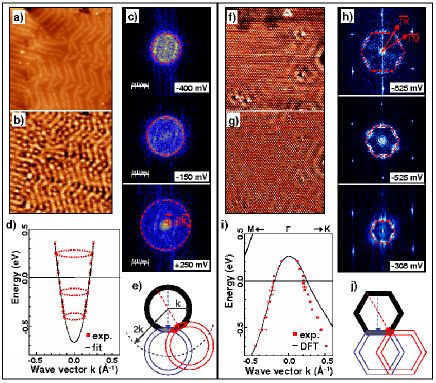
Figure 1: The STM picture a) shows the herringbone reconstruction of the Au(111) surface island, perturbed by a nearby dislocation ($50\times 50nm$, -0.4 V). b) is the dI/dV map of the topographic image a). Three 2D-FFTs of these dI/dV maps (with the corresponding applied bias) are shown in c), from which we get the energy dispersion curve of Au(111) shown in d). f) Topographic and g) dI/dV map at -30 meV ($20\times 20nm$) showing both standing waves and atomic resolution on $ErSi_{2}$ islands on Si(111). Three 2D-FFTs of these dI/dV maps (with the corresponding applied bias) are shown in h), from which we get the energy dispersion curve of $ErSi_{2}$/Si(111) shown in i). e) and j) represent the geometrical construction to get access to the density of scattering events of a CEC for gold and erbium disilicide respectively.

A first experimental illustration of the FT-STS technique is described in figure 1 for Schockley states probed on Au(111) surface. In a) the topographic STM image shows the herringbone reconstruction, and many defects (scatterers) are visible on the surface. The dI/dV map taken with a lock-in amplifier allows to measure directly the energy-resolved local density of states at several energies. We do not limit our analysis at the Fermi energy, but we analyze several different energies. When we perform the Fourier transform (here the power spectrum) of the different dI/dV images at increasing bias voltage we observe (in c)) a circle which increases in size. The radius of the circle corresponds to the $\mid\overrightarrow{q}\mid=2\mid\overrightarrow{k}\mid$ as shown in the geometrical construction e). We report the value of $q$ as a function of energy, which yields directly the dispersion curve, which is here parabolic, as expected in the case of a quasi ”free” electron gas. This is a direct proof of the susceptibility singularity at momentum $\mid\overrightarrow{q}\mid=2\mid\overrightarrow{k}\mid$.

This construction can be generalized for non circular CECs. In the right part of figure 1, for comparison we show the FT-STS for a two dimensional electron gas of $ErSi_{2}$. The system investigated here is the Erbium disilicide grown on Si(111)-7x7. This system has been extensively studied theoretically and experimentally by photoemission StaufferPRB93 ; WetzelSSCom92 , and an atomic model of this structure has been determined by Gewinner and co-workers TuilierPRB94 ; StaufferPRB93 . This structural model consists in a p(1x1) plane of Erbium atoms inserted between the silicon substrate and a buckled silicon layer WetzelSSCom92 . This system leads to a perfect 2D metal-semiconductor interface which shows a semi-metallic character with a hole pocket centered around the center of the surface Brillouin zone $\overline{\Gamma}$ and six electron pockets around the $\overline{M}$ symmetry points at the Fermi level. As shown in figure 1.i) the expected dispersion is ”hole-like” because it shows a reversed parabolic dispersion indicating a ”negative” effective mass. Indeed, contrary to the case of Au(111) surface, the size of the feature in the FT decreases when approaching the Fermi level.

In f) and g) we show typical topographic and dI/dV map images with point defects and standing waves pattern. Here the waves are non longer circular but have a hexagonal shape. In h) the power spectrum shows clearly a hexagon whose size decreases when approaching the Fermi level. The direct consequence of this CEC topology and of the fact that the susceptibility is $\overrightarrow{q}$ dependent, is the reinforcement of intensity along specific directions. Indeed along $\overline{\Gamma M}$ the FT is brighter than along $\overline{\Gamma K}$. While at first glance it may seem that this could be an effect of the form of the matrix elements in the scattering process, it can however be explained entirely by the topology in the CECs. As schematized in figure 1.i), the number of $\overrightarrow{q}$ vectors corresponding to the scattering events at the susceptibility singularity can be symbolized by the area of the intersection between two CECs translated by $q=2k$. For a circular contour this area is the same in all directions of the momentum space (as schematized in e) ), while for the hexagonal one this area is bigger in the $\overline{\Gamma M}$ direction (blue arrow) than in the $\overline{\Gamma K}$ direction (red arrow).

III.3 The joint density of states approximation

In a previous paper simonJCondMat07 we have formally established that the FT of a standing waves pattern image could be approximated by a joint density of states calculation (JDOS). In the presence of defects, the quasiparticles in the Bloch state $\overrightarrow{k}$ can be scattered into the Bloch state $\overrightarrow{k^{\prime}}$, and new eigenstates can be constructed, in perturbation theory, as linear combinations of the degenerate unperturbed states $\overrightarrow{k}$ that belong to the constant energy contour $E(k)=\omega$. The leading term in the Fourier component of the LDOS at wave vectors: $\vec{q}=\vec{k}^{\prime}-\vec{k}+\vec{G}$, where $\vec{G}$ is a reciprocal lattice vector, has an amplitude which takes the general form

$$g(\omega,\vec{q})=\frac{1}{{4\pi^{2}}}\!\!\!\!\!\!\iint\limits_{E(k)=E(k^{\prime})=\omega}\!\!\!\!\!\!\!\!\!\!{f(\vec{k},\vec{k}^{\prime},\vec{G})\delta(\vec{q}-\vec{k}+\vec{k}^{\prime}\pm\vec{G}})d^{2}\vec{k}\,d^{2}\vec{k}^{\prime}$$ (3)

where $f(\overrightarrow{k},\overrightarrow{k^{\prime}},\overrightarrow{G})$ is a weighting factor that depends on scattering matrix elements, and thus on the overall distribution and nature of defects.

The function $g(\omega,\overrightarrow{q})$ gives the joint density of states with a main contribution for $\overrightarrow{G}=0$ and replicas shifted by $\overrightarrow{G}$. The quantity $g(\omega,\vec{q})$ may be calculated by solving the Schrödinger equation for simple-defect geometries. Yet, if many defects of various symmetries are present, one may assume that $f(\overrightarrow{k},\overrightarrow{k^{\prime}},\overrightarrow{G})$ is a fairly smooth, slowly varying function of $\overrightarrow{k}$ and $\overrightarrow{k^{\prime}}$. Thus, practically in the JDOS approximation, $g(\omega,\vec{q})$, which is related to the power spectrum of the LDOS, could be calculated by performing the self correlation function of the CEC at a given energy. In practice, the JDOS calculations consist in counting the number of pairs of $\overrightarrow{k},\vec{k}^{\prime}$ wave vectors, yielding a scattering wavevector $\vec{q}$ with the same length and direction. We fabricate an image where the pixels position is defined by the wavevector $\vec{q}$, and the grey contrast is proportional to the number of the corresponding wavevectors pairs $\vec{k},\vec{k}^{\prime}$. This is a simple phenomenological approach of the generalization of the Lindhard susceptibility to Bloch waves states as developed by Blandin Blandin .

The figure 2 illustrates the fact that not only the structure, but also the shape of the features observed in the power spectrum, could be interpreted with a simple JDOS approach. In a) and b) are represented the CECs, the measured and theoretical band dispersion of the $ErSi_{2}$ system respectively. Up to -250meV (rectangular red box in b)), the CEC is split into two types of contours, the hole-like band structure previously discussed in Fig.1 and, crossing the Fermi level from unoccupied states, six ellipsoidal electron pockets emerging around the $M$ points. In the JDOS interpretation of the FTs, we should consider both the scattering processes joining hole-like and electron-like pockets (red arrow in a)), as well as scattering between the ellipsoidal electron-like pockets (blue arrow). Both should yield features centered around the $M$ points.

By changing the bias voltage in this energy range, the position of the feature does not change but only the shape. In c) we show the FT obtained at the Fermi level. One of the features arising in the FT is highlighted, and we can see that it has a ”butterfly” shape. We have found that this particular shape is associated to the self correlation between two CECs, a central circle (the hole band) and an elliptic electron pocket, i.e. it is the result of the scattering events schematized by the red arrow in a). The JDOS calculation for electron-electron scattering is also showed in c). This clearly demonstrates that the leading scattering event joins hole-like and electron-like pockets.

The dispersion relation as obtained from the FT-STS measurements is reported in b). This relation was deduced from the modification of the feature size with the bias voltage VonauPRL05 . An excellent agreement between our experimental points and previous ARPES measurements WetzelSSCom92 is found. The agreement is also excellent with the calculated band structure from Rogero et al. RogeroPRB04 in the direction $\overline{\Gamma M}$, but not in the direction $\overline{\Gamma K}$. Obviously, the $YSi_{2}$ DFT-LDA calculation reproduces the global shape of the measured hole band but the higher-energy excitations are shifted by values as large as $250$ meV. Similar shifts for the predicted surface-state energy positions around the $K$ point have been mentioned before for $YSi_{2}$ and $GdSi_{2}$ and the necessity to improve LDA self-energy term has been noted RogeroPRB04 .

The case of similar dispersing CECs for high $T_{C}$ superconductors has been studied in detail (see e.g. McElroyNature03 ; Vershinin2004 ), and more recently, for $Bi_{2}Sr_{2}CaCu_{2}O_{8+\delta}(Bi2212)$, the relationship between the ARPES measurements and the quasiparticule scattering interpretation of FT-STS measurement has been done using the concept of JDOS MarkiewiczPRB2004 ; K. McElroyPRL2006 . A more thorough theoretical approach to interpret these results, based on a Green function formalism, has been proposed by Wang and Lee QiangPRBR03 . Thus one can link the two measurement techniques yielding the real space single particle spectra for the STM and LDOS measurements, and the momentum space single particle spectral function for the ARPES measurements K. McElroyPRL2006 . To summarize, as the first order stationary perturbation theory is invoked in the JDOS approach, and as large signal-to-noise ratio is expected with this technique it is crucial to apply it to physical systems in which the scattering processes mix sufficiently the unperturbed wave functions in k-space and in energy. It has been discussed in detail by Capriotti et al. capriottiPRB03 , by Kodra and Atkinson KodraPRB06 , and for the case of high $T_{C}$ superconducting materials HoffmanScience02 ; McElroyNature03 . We note that this technique has been successfully applied even more recently for $GaN(0001)$ Sun2010 .

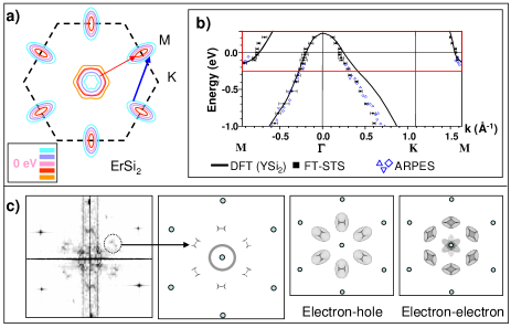
Figure 2: Constant Energy Contours of $ErSi_{2}$ in the energy region where both hole and electron band coexist (-200 meV to + 200 meV). b) shows the experimental band structure of $ErSi_{2}$ determined with ARPES and FT-STS measurements. The band structure is compared to DFT calculation of $YSi_{2}$. c) from left to right : Fourier transform of an STM image of $ErSi_{2}$. The dominating structures observed in M can be modelized by JDOS construction as depicted in Fig 1. JDOS calculations showing the contribution of different scattering events: the third frame shows the scattering events between the hole-like band and the electron-like band whereas the fourth frame displays the structure obtained by only electron-like band scattering.

III.4 Beyond the JDOS approximation - the stationary-phase approximation

Besides the electron-hole scattering processes, one should also take into account the hole-hole and electron-electron scattering events. At first glance, the predominance of electron-hole scattering events seems to be the effect of hidden matrix elements included in the function $f(\overrightarrow{k},\overrightarrow{k^{\prime}},\overrightarrow{G})$ in the expression of the JDOS (equation 3). However we can show that a simple interpretation can already be provided using the background theory of the susceptibility.

Up to now we have considered the steady states and neglected the phase factors in the rough JDOS approximation. In order to take into account these phase factors, the method of the stationary phase approximation is usually applied. It consists in noting that in the integral of the JDOS formula, oscillatory term with rapidly-varying phase will cancel, while the terms with the same phase should be added together. This leads to a supplementary criterion in the geometrical construction of the JDOS, similar to the case of the Kohn anomaly. As illustrated in figure 3.a) and along the lines of Ref. Blandin , we consider that the leading scattering process take place for values of the $\vec{q}$ momenta joining points of the CECs for which $\overrightarrow{\nabla_{k}(E(k))}$, $\overrightarrow{\nabla_{k^{\prime}}(E(k^{\prime}))}$ (or alternatively the tangents to the CECs) are parallel and point in the same direction.

In b) we consider a CEC similar to the Fermi surface of the Erbium disilicide with the central circle and the six ellipses. The full calculation of the JDOS is given in c) where we can easily recognize the features associated to the hole-electron and electron-electron scattering processes. By applying however the above-described criterion in our calculation we have obtained the JDOS given in d). Only the ”butterfly” features are preserved in the resulting spectra. This shows the importance of the phase factor, as well as that the matrix elements have no real effect on the FT features. This experimental result also nicely demonstrates the ”stationary phase” mathematical theorem.

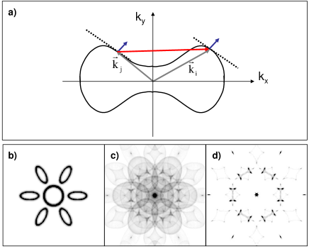
Figure 3: a) Representation of the stationary phase (blue parallel vectors) of a scattering event (red vector) resulting from the scattering from one state to another (depicted by the grey wave vectors) Blandin . b) CEC from erbium disilicide, and in c) the corresponding JDOS calculation. d) shows the dominating structures from c), when the stationary phase condition is taken into account; the result is in good agreement with the experimental FFT from Fig. 2.a).

IV FT-STS measurements on graphene and the T-matrix approximation

IV.1 T-matrix approximation

The T-matrix approximation has been successfully used to calculate the effects of disorder on the spectral properties of an electronic system. The basic theory is described for example in Mahan2000 ; Bruus2005 , and for a few example of how this is applied we mention Refs. Byers1993 ; Salkola1996 ; Ziegler1996 ; Hirschfeld1988 ; Polkovnikov2001 ; Podolsky2003 ; dhl ; ddw ; benakivelson ; benaprl ; Wehling2007 ; Peres2007 ; Peres2006 ; Vozmediano2005 ; Ando2006 ; Pogolerov ; Skrypnyk2006 ; Skrypnyk2007 ; Katsnelson2008 . The basic principle of this technique lies in an infinite perturbative summation of the diagrams resulting from expanding perturbatively the Green’s function of a system to all orders in the impurity scattering. In order to be able to apply the T-matrix approximation one needs to have the exact form of the tight-binding Hamiltonian of a system. The T-matrix approximation is valid as long as the impurity potential considered is localized, since it is this condition that allows the re-summation of all orders in perturbation theory. For extended impurities, the T-matrix approximation is in general replaced by the Born approximation, for which only the first order term in the impurity potential series is considered; this is equivalent to a perturbative expansion in the impurity potential which is valid only when the impurity scattering is weak. Nevertheless, both the T-matrix approximation and the Born approximation yield the same dependence of the DOS on position, what is different is the dependence of the DOS with energy, which is not the main point of our analysis.

IV.2 T-matrix approximation in momentum space

We will briefly review here the principle of the T-matrix approximation Mahan2000 ; Bruus2005 . The impurity scattering problem can be solved both in the real space and in momentum space. We will first focus on the momentum space calculation. For a given system one can define a finite temperature (imaginary time) generalized Green’s function,

$$G(k_{1},k_{2},\tau)=-{\rm Tr}\,e^{-\beta(K-\Omega)}\,{\rm T}_{\tau}\,\psi_{k_{1}}(\tau)\psi^{+}_{k_{2}}(0),$$ (4)

where $K=H-\mu N$, $e^{-\beta\Omega}={\rm Tr}\,e^{-\beta K}$, and ${\rm T}_{\tau}$ is the imaginary time ordering operator. For a translationally-invariant, disorder-free system the generalized Green’s function defined above is non-zero only if $k_{1}=k_{2}$ (momentum is conserved), and the generalized Green’s function reduces to the standard Green’s function which depends only on one momentum. However, the generalized Green’s function acquires a non-zero component for $k_{1}\neq k_{2}$ if the system is inhomogeneous, such as in the presence of impurity scattering. This component can be calculated using the $T$-matrix formulation dhl ; ddw ; benakivelson ; benaprl :

$$G(k_{1},k_{2},i\omega_{n})=G_{0}(k_{1},i\omega_{n})T(k_{1},k_{2},i\omega_{n})G_{0}(k_{2},i\omega_{n}),$$ (5)

where

$$G_{0}(k,i\omega_{n})=(i\omega_{n}-{\cal H}_{k})^{-1},$$ (6)

is the unperturbed Green’s function of the homogenous system, ${\cal H}_{k}$ is the Hamiltonian, and

$$T(k_{1},k_{2},i\omega_{n})=V(k_{1},k_{2})$$

$$+\sum_{k^{\prime}}V(k_{1},k^{\prime})G_{0}(k^{\prime},i\omega_{n})T(k^{\prime},k_{2},i\omega_{n}).$$ (7)

As detailed in Fig. 4, this expression stems from a perturbative expansion to all orders in the impurity scattering. If only the first term of the expansion is preserved, one recovers the first order perturbation theory in the impurity scattering potential, also denoted the Born approximation.

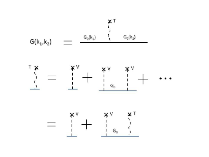
Figure 4: Diagrammatic description of the T-matrix approximation: the Green’s function for a system in the presence of an impurity can be obtained from adding to the unperturbed Green’s function the contributions corresponding to all-order impurity scattering processes. We note that the sum of the contributions appearing to the right of $G_{0}$ is identical to $T$, which allows one to write the self-consistency equation on the third line.

Oftentimes, one assumes that the impurity scattering potential is very close to a delta function so that $V$ is independent of $k$ and $k^{\prime}$

$${\cal H}_{imp}=\int dxVc^{\dagger}(x)c(x)\delta(x)=\int_{\vec{k},\vec{k}^{\prime}}Vc^{\dagger}({\vec{k}})c({\vec{k}^{\prime}})$$ (8)

For this case we can solve Eq. (7), and obtain

$$T(i\omega_{n}) = [1-V\int\frac{d^{2}k}{S_{BZ}}G_{0}(k,i\omega_{n})]^{-1}V$$ (9)

where $S_{BZ}$ is the area of the first Brillouin zone (BZ) of the system, and the integral over $k$ is performed over the entire Brillouin zone.

In the neighborhood of the impurity, spatial oscillations of the local density of states are induced. The Fourier transform of these oscillations can be related to the generalized Green’s function,

$$\rho(q,\omega)=i\sum_{k}g(k,q,\omega),$$ (10)

where $g(k,q,\omega)\equiv G(k,k+q,\omega)-G^{*}(k+q,k,\omega)$, and $G(k,k+q,\omega)$ is the generalized retarded Green’s function obtained by analytical continuation $i\omega_{n}\rightarrow\omega+i\delta$ from the Fourier transform of the imaginary-time Green’s function $G(k,k+q,i\omega_{n})$.

IV.3 T-matrix approximation in real space

If one is interested in the real space spectral properties of a system, such as the space dependence of the LDOS, one can use the real space T-matrix formalism. The relations described above can be Fourier transformed to real space, yielding for the retarded space-dependent generalized Green’s function of the system

$$G(\vec{R}_{1},\vec{R}_{2},E)=\int_{\vec{R}}{G}_{0}(\vec{R}-\vec{R}_{1},E)T(\vec{R},E){G}_{0}(\vec{R}_{2}-\vec{R},E)$$ (11)

where $T(\vec{R},E)$ is the space-dependent $T$-matrix. Same as for the momentum-dependent formalism, the generalized Green’s function depends on two (spatial) variables. In the absence of disorder, for an homogeneous system it is only a function of the difference $\vec{R}_{1}-\vec{R}_{2}$, so that only one spatial index is preserved in the notation: $G_{0}(\vec{R}_{1},\vec{R}_{2},E)\equiv G_{0}(\vec{R}_{1}-\vec{R}_{2},E)$. However, in the presence of disorder, the generalized Green’s function will depend on both variables independently.

The spatial dependent Green’s function characterizes the propagation between two points in space $\vec{R}_{1}$ and $\vec{R}_{2}$. If one is not interested in propagation of a particle between two spatial points, but would rather want to determine the spectral properties, for example the number of allowed states having a given energy at a given position, one needs to focus only on the limit $\vec{R}_{1}=\vec{R}_{2}=\vec{r}$. Consequently, the LDOS can be obtained from the retarded Green’s function by using the conventional relation:

$$\rho(\vec{r},E)=-{\rm Im}G(\vec{r},\vec{r},E)$$ (12)

In general one focuses on a delta-function impurity localized at $\vec{R}=0$, which yields

$$G(\vec{r},\vec{r},E)={G}_{0}(-\vec{r},E)T(E){G}_{0}(\vec{r},E)$$ (13)

where $T(\omega)=[1-V\int\frac{d^{2}\vec{k}}{S_{BZ}}{G}_{0}(\vec{k},\omega)]^{-1}V,$ and the integral over $\vec{k}$ is performed on the first BZ, whose area is denoted as $S_{BZ}$.

IV.4 Graphene FT-STS fundamentals

The Fourier-transform spectroscopy has begun to be widely used also for graphene systems. Beyond the fascinating properties of this system and the richness of the possible fundamental studies, graphene is for us an interesting system particularly for its band structure and for the CEC contour topology at specific energies, which provide a good testing ground for the validity of the FT-STS technique. Figure 5 recalls the key feature of the band structure of graphene. The CECs (given in a)) start from Dirac points around K points as circular contours which become triangular with increasing energy until the contours touch together at the $M$ points at the so called Van Hove singularities (VHs). These points are indicated in the CEC map, on the 3D view of the band structure (given in b)), and on the corresponding density of states. In d) we have schematized the CEC map for an energy near the Dirac point and the possible scattering events expected in the presence of impurities.

Graphene layers have two inequivalent atoms par unit cells. This is one of the key properties of the graphene. For this reason graphene should be described by two Bloch waves families, and the K points are inequivalent (non-equivalent wave vectors denoted K and K’). Around these K points, and close to zero energy, it has been showed that an effective Hamiltonian could be defined as Castroneto2009 :

$$H_{K}=v_{F}\mathbf{\sigma}.\mathbf{p}$$

where $\mathbf{\sigma}$, denoted pseudospin, is an operator which generates the transformation $H_{K}=-H_{K^{\prime}}$. The pseudospin provides a supplementary quantum number defined only at low energy in the immediate vicinity of the K points. The pseudospin is symbolized by the blue and red arrows in d). As previously discussed for Erbium disilicide, the expected allowed scattering $\vec{q}$ wave-vectors could join two points of the same isocontour (intra-valley scattering) leading to a circle centered at $\Gamma$, or join two different valleys (inter-valley scattering). The first type of scattering leads to long wavelength oscillations in real space, while the second one leads to the well known short wavelength reconstruction observed in the vicinity of point defects in graphene, and to the $\sqrt{3}\times\sqrt{3}$ reconstruction oftentimes reported for graphite and graphene around point defects RuffieuxPRL00 ; RuffieuxPRB05 and more recently near step edges DujardinNanolett10 .

However, as we will describe in more details in the next section, not all scattering processes are allowed for graphene. Since the pseudospin acts as an extra quantum number, two waves of opposite pseudospin cannot interfere and generate standing waves. Thus, since for two points on a CEC having opposite momenta relative to a K point, the pseudospins are opposite, the intra-valley backscattering is expected to be suppressed. However this is not the case in a backscattering event $\overrightarrow{K}$, $\overrightarrow{-K}$ connecting two different opposite K valleys.

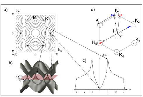
Figure 5: A three-dimensional (3D) representation of the band structure of graphene, and a plot of the constant-energy contours. a) The constant energy contours starting from the Dirac point, calculated in the nearest-neighbor tight-binding approximation. The key features of the band structure, the Dirac points and the Van Hove singularities are indicated on the 3D representation in b), and on the theoretical density of state in c). The expected intra- and inter-valley scattering processes and the corresponding pseudospin orientations (as discussed in the text) are schematized in d)

In the following we will see how the FT-STS technique could be useful to probe and analyze the quantum nature of the quasiparticles on graphene, and how the interpretation of the FT can be done using the T-matrix approximation.

IV.5 The Hamiltonian and Green’s functions for monolayer and bilayer graphene

The momentum-space tight-binding Hamiltonian for monolayer graphene graphene is:

$${\cal H}=\int d^{2}\vec{k}[a_{\vec{k}}^{\dagger}b_{\vec{k}}f(\vec{k})+h.c.],$$ (14)

where the operators $a^{\dagger}$, $b^{\dagger}$ correspond to creating electrons on the sublattice $A$ and $B$ respectively, and $f(\vec{k})=-t\sum_{j=1}^{3}\exp(i\vec{k}\cdot{\vec{a}_{j}})$. Here $\vec{a}_{1}=a(\sqrt{3}\hat{x}+\hat{y})/2$, $\vec{a}_{2}=a(-\sqrt{3}\hat{x}+\hat{y})/2$, $\vec{a}_{3}=-a\hat{y}$, $t$ is the nearest-neighbor hopping amplitude, and $a$ is the spacing between two adjacent carbon atoms, which we are setting to $1$.

This form of the Hamiltonian has been used in Ref. benaprl to perform a numerical analysis of the FT-STS spectra. It is also useful to expand the Hamiltonian close to the corners of the BZ, which we also denote as nodes or “Dirac points”, and use the linearized form to solve the problem analytically at low energies benaprl . The momenta of the six corners of the Brillouin zone are given by $\vec{K}_{1,2}=[\pm 4\pi/(3\sqrt{3}),0]$, $\vec{K}_{3,4}=[\pm 2\pi/(3\sqrt{3}),2\pi/3]$, $\vec{K}_{5,6}=[\pm 2\pi/(3\sqrt{3}),-2\pi/3]$. Close to each corner, $m$, of the BZ we can write $f(\vec{q}+\vec{K}_{m})\approx\tilde{\phi}_{m}(\vec{q})=v_{m}\vec{q}\cdot\vec{J}_{m}$, where $\vec{q}$ denotes the distance from the respective corner. Also $v_{1,2}=3t/2=v$, $v_{3,4}=v\exp(-i\pi/3)$, $v_{5,6}=v\exp(i\pi/3)$ and $\vec{J}_{1,2}=(\pm 1,-i)$, $\vec{J}_{3,4}=\vec{J}_{5,6}=(\pm 1,i)$.

The corresponding Green’s function, ${\cal G}(\vec{k},\omega)$, derived from the tight-binding Hamiltonian in Eq. (14) can be expanded at low energy around the six nodes (denoted $m$), and in the $2\times 2$ (A,B) sublattice basis can be written as:

$${\cal G}(\vec{k},\omega)\approx G_{m}(\vec{k},\omega)=\frac{1}{\omega^{2}-|\tilde{\phi}_{m}(\vec{k})|^{2}}\begin{pmatrix}\omega+i\delta&\tilde{\phi}_{m}({\vec{k}})\\ \tilde{\phi}_{m}^{*}(\vec{k})&\omega+i\delta\end{pmatrix}$$ (15)

where $\delta$ is the quasiparticle inverse lifetime. The Fourier transform of the linearized Green’s function is given by benaprl :

$$G_{m}(\vec{r},\omega)\propto\omega\begin{pmatrix}H_{0}^{(1)}(z)&i\phi_{m}(\vec{r})H_{1}^{(1)}(z)\\ i\phi^{*}_{m}(\vec{r})H_{1}^{(1)}(z)&H_{0}^{(1)}(z)\end{pmatrix}$$ (16)

where $z\equiv\omega r/v$, $H_{0,1}^{(1)}(r)$ are Hankel functions, $r=|\vec{r}|$, and $\phi_{m}(\vec{r})=v_{m}\vec{r}\cdot\vec{J}_{m}/(vr)$.

On the other hand, the bilayer graphene consists of two graphene layers stacked on top of each other such that the atoms in the sublattice $A$ of the first layer occur naturally directly on top of the atoms in the sublattice $\tilde{B}$ of the second layer vanMieghem1992 ; McCann2006 , with a tunneling coupling of $t_{p}$.

In the sublattice basis $(A,\tilde{B})$ this yields McCannPRL2006 ; Nilsson2006 :

$${\cal H}^{bilayer}_{m}(\vec{k})=\begin{pmatrix}0&[\tilde{\phi}_{m}(\vec{k})]^{2}\\ [\tilde{\phi}_{m}^{*}(\vec{k})]^{2}&0\end{pmatrix}$$ (17)

where for simplicity we have set the effective mass of the quadratic spectrum to $1$. The corresponding Green’s function in real space is given by:

$$G_{m}(\vec{r},\omega)\propto\begin{pmatrix}H_{0}^{(1)}(z)&-[\phi_{m}(\vec{r})]^{2}H_{2}^{(1)}(z)\\ -[\phi^{*}_{m}(\vec{r})]^{2}H_{2}^{(1)}(z)&H_{0}^{(1)}(z)\end{pmatrix}$$ (18)

where we denoted $z=r\sqrt{|\omega|}/v$.

IV.6 Calculations of the FT-STS for graphene using the T-matrix

Ref. benaprl focuses on monolayer graphene, with a delta-function impurity localized on an atom belonging to sublattice $A$. In the $(A,B)$ basis the impurity potential matrix $V$ has only one non-zero component $V_{11}=u$. The T-matrix formalism presented above can be generalized to graphene for which the Green’s functions and the T-matrix for graphene become $2\times 2$ matrices, such that

$$G(k_{1},k_{2},i\omega_{n})={\cal G}_{0}(k_{1},i\omega_{n})T(k_{1},k_{2},i\omega_{n}){\cal G}_{0}(k_{2},i\omega_{n}),$$ (19)

and where

$${\cal G}_{0}(k,\omega)^{-1}\propto\begin{pmatrix}\omega+i\delta&f(k)\\ f^{*}(k)&\omega+i\delta\end{pmatrix}$$ (20)

and $T(\omega)=[I-V\int\frac{d^{2}\vec{k}}{S_{BZ}}{\cal G}(\vec{k},\omega)]^{-1}V,$ where $I$ is the $2\times 2$ identity matrix, and the integral over $\vec{k}$ is performed on the BZ, whose area is $S_{BZ}=8\pi^{2}/3\sqrt{3}$.

At arbitrary energy this cannot be calculated analytically, but can be analyzed numerically benaprl , and the resulting FT-STS spectra (corresponding to the real part of the Fourier transform of the LDOS) are plotted in Fig. 6.

Figure 6: FT-STS spectra for a monolayer graphene sample with a single delta-function impurity. Fig. a) corresponds to energies $0.15t$ at $\delta=0.07t$. The actual lowest ($0$) and highest ($1$) values of the FT-STS intensity are $(-1.3,2.6)$ in arbitrary units. Fig. b) shows a cross section of the FT-STS intensity as a function of $k_{x}$ for $k_{y}=0$ for energy $0.15t$.

The calculation shows regions of high intensity in the FT-STS spectra corresponding to intranodal quasiparticle scattering (central region) and internodal scattering (outer regions). The central high-intensity region is a filled circle, while the outer regions are empty. Also, the rotational symmetry of the high-intensity regions located at the corners of the BZ is broken.

We can compare this result to the one obtained by the joint density of states (JDOS) formalism. The JDOS formalism focuses mainly on the position in k-space of the quasiparticle peaks at a given energy, and considers that scattering takes place equally between all quasiparticles living at a given energy. Formally this is equivalent to writing

$$\rho(q,i\omega_{n})=\int_{k}{\rm Im}\{{\rm Tr}[G_{0}(k,i\omega_{n})]\}V{\rm Im}\{{\rm Tr}[G_{0}(k+q,i\omega_{n})]\},$$ (21)

We can see that in this formalism neither the chiral structure of the Hamiltonian of graphene, nor the phase of the matrix elements are taken into account, and one focuses solely on the eigenvalues of the Hamiltonian. The loss of information is evident when in Fig. 7 we plot the JDOS result for graphene:

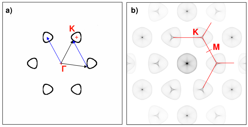
Figure 7: In b) the FT-STS map for a monolayer graphene calculated using the JDOS approximation for the CEC given in a). The arrows in b) show the inter-valley scattering momenta leading to the feature observed around the K points in b). The central circle corresponding to intra-valley scattering does not appear in the T-matrix calculation, and is not observed experimentally. As detailed in the text, this is a consequence of the chirality of graphene quasiparticles.

Indeed here the calculated FT-STS shows a central circle corresponding to the intravalley scattering which is not obtained in the T-matrix calculation, nor observed experimentally. The feature observed in the middle of each K contour (inter-valley scattering) is due to the trigonal warping of the contour.

For bilayer graphene, in Ref. benaprl , one has considered the case of an impurity located on the sublattice $A$. The resulting FT-STS spectra for the LDOS in the top layer are presented in Fig. 8.

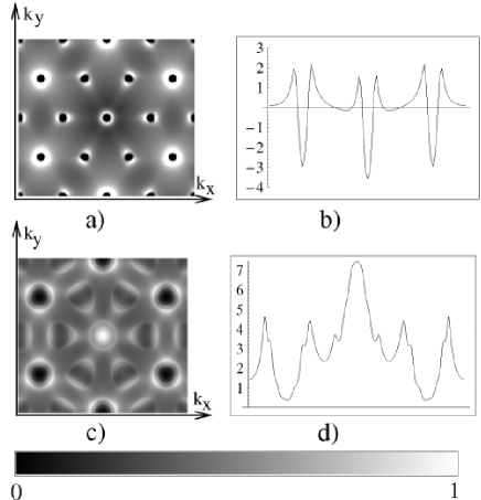
Figure 8: FT-STS maps for a bilayer sample. Figs. a) and c) depict the FT-STS intensity in arbitrary units at energies $0.1t$, $0.4t$, with $t_{p}=0.3t$, and $\delta=0.05t$. The actual lowest ($0$) and highest ($1$) values of the FT-STS intensity are $(-6.9,3.6)$ and $(-6.0,7.4)$ respectively. Figures b) and d) are cross-sections at $k_{y}=0$ of Figs. a) and c).

There are similarities and discrepancies between the monolayer and bilayer cases. Like in the monolayer case, there are areas of high intensity centered on the center and corners of the BZ. The main difference at low energy is that the central region of high intensity is an empty circle, and not a full circle (as for the monolayer case). At high energy, we also note a doubling of the number of high intensity lines corresponding to the doubling of the number of bands.

IV.7 Calculations of the spatial dependence of the LDOS

We now turn to the study of the dependence of the LDOS on the relative position with respect to the impurity ($\vec{r}$). We note that a calculation of the LDOS at arbitrary energy can be performed numerically using Eqs. (12,13), where the real-space Green’s function for graphene can be calculated numerically by taking a FT of the full k-space Green’s function of graphene in Eq. (6). However, at low energies, the physics is dominated by linearly dispersing quasiparticles close to the Dirac points, and the calculation can be performed analytically. The spatial variations of the LDOS due to the impurity have been found to be benaprl :

$$\rho(\vec{r},E)\propto-{\rm{Im}}[{\cal G}(-\vec{r},E)T(E){\cal G}(\vec{r},E)]\approx-\sum_{m,n}{\rm{Im}}[e^{i(\vec{K}_{m}-\vec{K}_{n})\cdot\vec{r}}G_{m}(-\vec{r},E)T(E)G_{n}(\vec{r},E)],$$ (22)

where $m,n$ denote the corresponding Dirac points. Here $T(E)$ is again the $T$-matrix, which for a delta-function impurity is given by $T(\omega)=[I-V\int\frac{d^{2}\vec{k}}{S_{BZ}}{\cal G}(\vec{k},\omega)]^{-1}V,$ where $I$ is the $2\times 2$ identity matrix, and the integral over $\vec{k}$ is performed on the BZ, whose area is $S_{BZ}=8\pi^{2}/3\sqrt{3}$.

Using Eq. (16) and expanding the Hankel functions to leading order in $1/r$, in Ref. benaprl , it has been found that far from the impurity ($\omega r/v\gg 1$) the corrections to the local density of states due to scattering between the nodes $m$ and $n$ are given by:

$$\rho_{mn}(\vec{r},\omega)\propto\frac{\omega}{r}{\rm{Im}}\big{\{}t(\omega)e^{i(\vec{K}_{m}-\vec{K}_{n})\cdot\vec{r}+2i\omega r/v}i\big{[}1-\phi_{m}^{*}(\vec{r})\phi_{n}(\vec{r})\big{]}\big{\}}.$$ (23)

where $t(\omega)$ is the non-zero element of the $T$-matrix ($T_{11}$), as it was noted that $\phi(-\vec{r})=-\phi(\vec{r})$.

In the case of intranodal scattering ($m=n$) the above expression vanishes and the LDOS is dominated by the next leading correction $\rho_{m}(\vec{r},\omega)\propto\sin(2\omega r/v)/r^{2}$. This is different from what usual wisdom would suggest for a two-dimensional system ($1/r$ decay) benakivelson ; steveold , and has also been described in Refs. falko ; glazman .

As briefly outlined above in section Graphene FT-STS fundamentals, the underlying physics of this result stems from the chirality of the graphene quasiparticles Geim ; Katsnelson . The graphene quasiparticles, due to the presence of two atomic sublattices, have an additional degree of freedom deemed pseudospin, such that one says that a quasiparticle belonging to sublattice A has pseudospin “up”, and a quasiparticle belonging to the sublattice B has pseudospin “down”. By chirality, the pseudospin vector is parallel to the quasiparticle momentum, so that if we know the momentum of a quasiparticle, we automatically know its pseudospin, thus to which sublattice it belongs and in which proportion. Due to the chiral properties of the quasiparticles, backscattering of quasiparticles by extended impurities is forbidden Ando ; Katsnelson2 , because when a quasiparticle is backscattered flipping its momentum by $180^{\rm o}$, by chirality, its pseudospin also flips. Since an extended impurity cannot flip the pseudospin of an electron (the wavelengths associated with backscattering are much larger than the atomic lattice constant), the backscattering cannot take place. Nevertheless, if the impurity is localized, the backscattering is not forbidden Katsnelson3 . However, the incident and backscattered particle have opposite pseudopspins, and thus their wavefunctions cannot interfere constructively, same as the wavefunctions of two electrons with spin up and spin down cannot give rise to constructive interferences. This lack of interference yields a reduction of the Friedel oscillations in the vicinity of the impurity, which no longer decay as $1/r$ as in a regular two-dimensional electron gas, but much faster, as $1/r^{2}$.

We should note that the two-dimensional FT of $\sin(2\omega r/v)/r^{2}$ is roughly $\rho_{m}(q,\omega)\propto\pi\theta(2\omega-qv)/2+\arcsin(2\omega/qv)[1-\theta(2\omega-qv)]$. This corresponds to a filled circle of high intensity in the FT-STS spectrum, which is consistent with the results of our numerical analysis for the central region of high intensity.

Nevertheless, for the decay of the Friedel oscillations generated by internodal scattering ($m\neq n$), the chirality considerations are not longer applicable (quasiparticles close to different nodes have different chiralities), and the leading order behavior of the Friedel oscillations is $1/r$. The FT of $\cos(2\omega r/v)/r$ is $\theta(qv-2\omega)/\sqrt{q^{2}v^{2}-4\omega^{2}}$, which translates into empty circles of high intensity in the FT-STS spectra, consistent with our numerical analysis.

For bilayer graphene, an analytical study can be performed at low energies starting from the expansion of the Hamiltonian around the Dirac points $m$. Starting from Eq. (22), Ref. benaprl has performed a similar analysis to the case of monolayer graphene. It was noted that at large distances ($z\gg 1$), as opposed to the monolayer case, the leading ($1/r$) contribution for intranodal scattering is non-vanishing:

$$\rho_{m}(\vec{r},\omega)\propto\frac{1}{r\sqrt{|\omega|}}\cos(r\sqrt{|\omega|}/v).$$ (24)

This is consistent with the appearance of an empty circular contour at the center of the BZ, as opposed to the filled circle for the monolayer case. The leading contribution to the decay of the oscillations due to internodal scattering is also $1/r$.

IV.8 Experimental measurements of FT-STS in graphene

Experiments to measure the LDOS in graphene have been performed by quite a few groups mallet ; rutter ; benamallet ; benasimonEPJB ; cranneyEPL10 . Thus, for example, we present below some real-space images from Ref. benamallet , for graphene monolayer (Fig. 9.a)) and graphene bilayer (Fig. 9.b)). Note that both images exhibit a triangular pattern of periodicity $\sim$ 1.9 nm which is related to the interface reconstruction mallet ; rutter , and which appears as a sextuplet of bright spots in the corresponding FFT images([Figs. 9.c) and 9.d)). Also in Fig. 10, we present the LDOS and its Fourier transform as measured in Ref. benasimonEPJB .

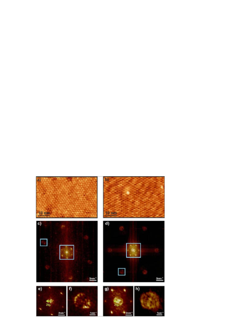
Figure 9: a),b) Low-bias STM images of 50 nm wide monolayer a) and bilayer b) terraces. Sample bias and tunneling current are respectively +2 mV and 0.4 nA for a), +4 mV and 0.13 nA for b). c), d) Two-dimensional fast Fourier transform (FFT) maps of the STM images a) and b). e) Central region of c), showing no intravalley-backscattering related ring (the green arrow points out the position where such a ring should appear). f) One of the outer pockets of c). g) Central region of d), showing a clear ring-like feature of radius 2$q_{F}$ related to intravalley-backscattering. h) One of the outer pockets of d). Outer pockets shown in f) and h) are centered at the $K$ (or $K$’) point and result from intervalley scattering. Data courtesy : I. Brihuega et al. benamallet .

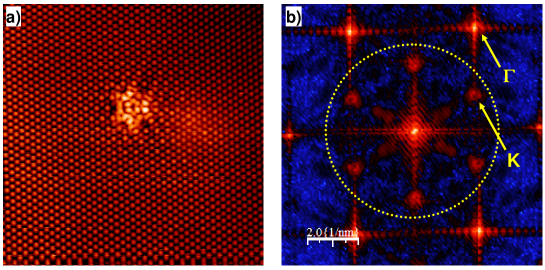
Figure 10: a) STM topographic image ($10\times 10nm^{2}$, -17$meV$, 1$nA$) showing an isolated defect. b) The FFT power spectrum of the 2D topographic image in a).The features indicated by the arrows correspond to inter-valley scattering.

The central region of the FFT in Figs. 9.c) and 9.d) is related to intravalley scattering: a clear ring-like feature of average radius 1.2 nm^-1 is found for the bilayer (Figs. 9.d) and 9.g)). This radius value is in agreement with the value given in ref. rutter , and with the 2$q_{F}$ value derived from ARPES Bostwick ; Zhou . On the monolayer terrace, no central ring is found (Figs. 9.c) and 9.e)), despite the unprecedented momentum resolution (the result has been checked on many different monolayer terraces). This corresponds to the presence of slowly-decaying ($1/r$) long-wavelength oscillations in bilayer graphene, but not in monolayer graphene.

In the high frequency regions of the FFTs of Figs. 9.c) and 9.d), six outer pockets with ring-like shapes centered at $K$($K^{\prime}$) points have been observed. They result from intervalley scattering, associated to real space LDOS modulations with a ($\sqrt{3}\times\sqrt{3})R30^{\circ}$ periodicity with respect to graphene mallet ; rutter . As shown in Figs. 9.f) and 9.h), the intensity of the high frequency rings in the FFT is not isotropic. The anisotropy is much more pronounced for graphene monolayer. The presence of the anisotropy is in agreement with the theoretical calculations of Ref. benaprl presented in Fig. 6.

The experiment described in benamallet thus confirms the theoretical picture presented in section Calculations of the FT-STS for graphene using the T-matrix, confirming the chiral properties of the graphene quasiparticles, and also that these properties can be probed at the nanometer scale using scanning tunneling spectroscopy.

IV.9 Determination of the band structure of graphene from the FT-STS spectra

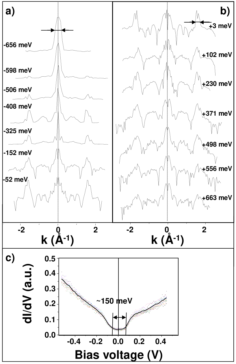
Figure 11: a), b) Intensity profiles along the $K-\Gamma-K$ direction of the 2D FT of the LDOS taken for different bias voltages. c) STS measurement taken near the impurity showing a gap centered around the Fermi level.

The Fourier transform of the LDOS can be used not only to extract information about the chirality of quasiparticles, as described above, but also about the quasiparticle energy dispersion (see for example McElroy2005 ; Vershinin2004 ; Fang2004 ; rutter ). In Fig. 11 we present intensity profiles along the $K-\Gamma-K$ direction for the Fourier transform of the LDOS at various energies benasimonEPJB . Every image was acquired using a lock-in amplifier and a modulation voltage of $\pm 20$ $meV$ which gave the energy uncertainty. For a wide range of energies, between energies well below the Fermi level ($-950$ $meV$) to about $-150$ $meV$, the width of the peak at the center of the Brillouin zone (measured at half maximum) shows a clear dispersion with the bias voltage (it decreases when the energy moves towards the Fermi level). At energies closer to the Fermi level the profile becomes more complex and displays a dip in the intensity profile close to the $\Gamma$ point. The central peak also shows two lateral structures (shoulders). The width of the central feature does not appear to disperse with energy close to the Dirac point, but it starts dispersing again for higher positive energies.

Fig. 12 shows a linear dependence of the width of the central feature with energy, except in an energy range from $-200$ $meV$ to $100$ $meV$. For these energies the shape of the central peak is more complex. Also, in this range of energy, Fig. 11.c) presenting the measurement of the LDOS as a function of energy taken close to the impurity, shows a $150$ $meV$ gap-like feature centered around the Fermi level at $0$ $meV$. The Dirac point is estimated at $-100$ $meV$ below the Fermi level. The spreading in the dispersion of the points close to the Fermi level could be attributed to the presence of the gap.

The width of the features at the K points follows a similar dispersion. Beyond $+500meV$, all the features seem to follow a different dispersion branch, as indicated in Fig. 12. In ref. benasimonEPJB a comparison between the experimental results with similar theoretical profiles obtained using a T-matrix approximation for a single localized impurity in bilayer graphene benaprl is also presented. No gap at the Fermi level was included in the theoretical calculation, while a small gap of $\approx 100$ $meV$ was assumed near the Dirac point, which was taken to be close to $-250$ $meV$. In Fig. 12.b) is plotted the dispersion of the central and K-points features, and of the shoulder, as obtained from the theoretical curves. One observes the presence of two different dispersion branches. The second dispersion branch and the shoulder arise because of the bilayer graphene upper band which opens at energies higher than the inter-layer coupling. For monolayer graphene these extra features should not appear.

Thus the measurements in benasimonEPJB show that the quasiparticle approximation and the Fermi liquid theory are robust over a large range of energies. The complex structure of the central feature (the existence of the shoulder), as well as the presence of two dispersion branches are consistent with the bilayer (or multilayer) character of the graphene sample. While the point defect modifies the electronic wave-function in its vicinity, a clear linear dispersion is still observed, and the relativistic character of the quasiparticle is preserved. Also, the STS measurements in Fig. 11.c) indicate the presence of a gap centered at the Fermi point, and not at the Dirac point inferred from our FT-STM measurements. This gap is thus different from the Dirac-point gap observed by ARPES Bostwick ; Zhou which was attributed to the different doping levels of the epitaxial graphene layers. It is however consistent with previous STM measurements performed on epitaxial graphene BrarAPL07 , and more recently on exfoliated graphene Crommie08 , where a gap observed at the Fermi level was attributed to a pinning of the tunneling spectrum due to the coupling with phonons.

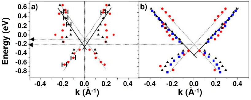
Figure 12: The dispersion for the width of the central-ring feature (red circles) and of the K-points feature (black triangles) obtained in a) from the experimental data from Fig. 11, and from the theoretical $K-\Gamma-K$ cuts (b)). The dispersion of the central-feature shoulder on the theoretical curves is indicated by blue squares.

IV.10 Measurement of the spatial dependence of the LDOS in the vicinity of a defect

Figure 13.a) shows a topographic image of a large graphene terrace taken at $-17$ $meV$ (probing filled states), as measured in Ref. benasimonEPJB . This layer shows an intriguing “star-like” defect with an apparent six-fold ($C6v$) symmetry. This atomic defect is accompanied by a strong distortion of the graphene lattice. The center appears black, which is a dramatic change from the case of the unperturbed lattice. As schematized in figure 13.c), a detailed analysis of the real-space image, shows that the point defect is directly located above or below a lattice site.

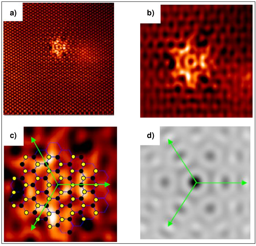
Figure 13: a) STM topographic image ($10\times 10nm^{2}$, -17$meV$, 1$nA$) showing an isolated defect. b) Zoom-in ($5\times 5nm^{2}$) on the defect, subsequent to a FFT filtering removing atomic resolution and second order features in the 2D FFT. c) $2.5\times 2.5nm^{2}$ zoom in on b) with the schematic atomic lattice of graphene (A/black and B/yellow atoms) superimposed over the standing waves pattern around the point defect. d) The real-space LDOS in a bilayer graphene calculated for a point defect using a single-impurity T-matrix approximation at $300meV$ above the Dirac point.

Using FFT filtering, Ref. benasimonEPJB has removed the lattice periodicity vectors and all other features with wavevectors outside the yellow circle in Fig. 10.b), thus taking into account only the intra-valley and the inter-consecutive-valley scattering processes. The resulting real-space image is shown in figure 13.b). This operation strongly enhances the anisotropic intensity observed also on the bare topographic image. The LDOS near the defect shows a clear threefold ($C3v$) symmetry. While, as depicted in Fig. 13.c), close to the impurity one observes a fairly homogeneous standing waves ring, with an almost perfect six-fold symmetry, farther away from the impurity, the intensity is clearly higher along three axes (drawn in green in Figs. 13.c) and 13.d)).

In Ref. benasimonEPJB the possible origin of this three-fold symmetry has been analyzed by comparing the theoretical LDOS for a point defect to the experimental data. The theoretical LDOS modulation for a bilayer graphene in the presence of a single impurity has been calculated using the real-space T-matrix formalism, modified to incorporate the finite spatial extend of the carbon electronic orbitals benaprb . The results for an energy of $300$ $meV$ above the Fermi level are presented in Fig. 13.d). One notes quite a few features similar to the ones depicted in Fig. 13.c), including the existence of a three-fold symmetry. However the three-fold anisotropy is much less pronounced.

Figure 14 displays the calculated real-space modulations in the LDOS close to the point defect, when only specific scattering processes have been considered. For simplicity this calculation has been performed for a monolayer graphene, as for bilayer graphene it is less clear how much the two bands and the two layers contribute to the measured LDOS. The intra-nodal scattering processes are responsible for radially-symmetric features with small $\overrightarrow{q}$ wavevectors and should therefore not be responsible for the presence of the three-fold symmetry.

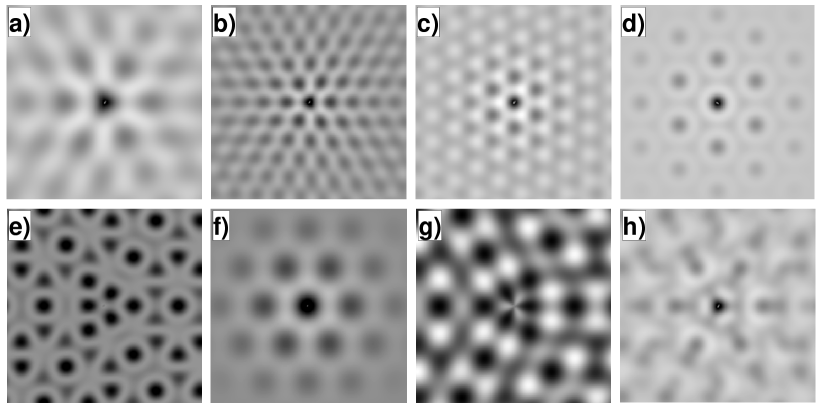
Figure 14: Calculated real-space LDOS modulations in a monolayer graphene for a point defect placed on top of an A atom. Figs. 14 a), b), c) depict the contributions of selected scattering processes to the LDOS ($K\rightarrow K_{1},K\rightarrow K_{2}$ and $K\rightarrow K_{3}$ respectively) as indicated in Fig. 5 d); Figs. 14 f), and g) depict the separate contributions of the A and B sublattices to the $K\rightarrow K_{1}$ LDOS modulations in a). Figs. 14 d) and e) depict the A and B sublattice contributions to the full LDOS, evaluated when all scattering processes are considered. In h) we depict the sum of the A and B contributions to the full LDOS, when the weight of the $K\rightarrow K_{1}$ B component is increased three times compared to that of the $K\rightarrow K_{1}$ A component.

Fig. 14.h) depicts the sum of the A and B contributions to the full LDOS, where in order to increase the anisotropy, the $K\rightarrow K_{1}$ B contribution has been multiplied by three. This may mimic bilayer graphene where, due to the coupling between the two layers, the sublattices A and B may not contribute equally to the observed LDOS. A very strong threefold symmetry is observed in this weighted superposition, and the resulting image corresponds more closely to the pattern observed experimentally in figure 13.b). This is consistent with having a defect at an A site whose dominant effect is the scattering of sublattice B electrons between two consecutive valleys ($K\rightarrow K_{1}$).

More recent experiments presented in Rutter2 indicate that in monolayer graphene patterns similar to the ones observed in benasimonEPJB but six-fold symmetry may arise as a result of rotating sequences of dislocations that close on themselves, forming grain boundary loops that either conserve the number of atoms in the hexagonal lattice or accommodate vacancy/interstitial reconstruction, while leaving no unsatisfied bonds. It would be interesting to generalize the results presented in Rutter2 to bilayer graphene to see if one can obtain similar patterns to the ones observed in benasimonEPJB .

IV.11 Van Hove extension deduced from FT-STS features on graphene modified by the intercalation of gold clusters.

The FT-STS technique has recently also been used to interpret the strong standing waves pattern observed on epitaxial monolayer (ML) graphene, modified by the intercalation of gold atoms. As described also above, epitaxial graphene on SiC(0001) consists of a buffer graphene layer which is covalently bonded with the substrate, and of a ML graphene weakly connected to the buffer layer. The monolayer graphene is n-doped with a transfer of electrons from the substrate. We have discovered that the deposition of gold atoms under UHV at room temperature, followed by an annealing cycle, leads to the intercalation of gold in different forms PremlalAPL09 . One of them is the intercalation of aggregates made of 1 to 3 small flat 6-atoms gold clusters. Figure 15 shows these results. In a) is shown a topographic image taken at -1V. The clusters appear under the graphene ML as bright spots. The dI/dV map image of the same area taken at $+0.9$V shows that the clusters appear as dark regions. As we probe here the empty states it seems that the aggregates create an excess of electron as schematized in d).

In between the gold clusters, a standing waves pattern develops, as revealed by bright p(2x2) protrusions, and the size of the dark regions decreases as the bias voltage increases cranneyEPL10 . These standing waves are associated to elliptic features in the FT-STS spectra, located around the M points as shown in c). The size of these elliptic features increases linearly with the bias voltage. Using the JDOS calculation we have deduced that these features are associated to the VHs cranneyEPL10 . In fact these elliptic features are observed in the JDOS spectra only when the CEC touch each other at the M point. This is shown in the calculated JDOS e) and h) for the CEC f) and g) respectively. In f) the contours do not touch each other, and no features are observed around M in e) while for h) as soon as the contours touch each other, an ellipse is observed.

This ellipse is associated to the k-vectors symbolized as blue arrows, which connect the apex of two consecutive triangular K contours (inter-valley scattering). The size of the ellipse is associated to the filling of the states located at the triangle apex. This indicates an extension of the VHs. This has been very recently confirmed by ARPES measurements in the occupied states tobepublished . Two other features in the perpendicular direction $\Gamma-M-\Gamma$ expected in both JDOS, and even in T-matrix approximation calculations are not observed experimentally. These features are associated to the wavevectors symbolized by the red arrows which should correspond to intra-valley scattering. As we are at large energies this could not be due to the pseudospin orientation. The possibility to a nodal-antinodal dichotomy has been discussed but remains under debate cranneyEPL10 . The reasons why the clusters create such an VHs extension remains non understood. We have recently shown that a change in the third nearest neighbor hopping energy in the tight-binding Hamiltonian create strong modifications of the band structure around the M points and even give rise to new Dirac points benasimonPRB2011 , but the experimentally observed third-nearest neighbor coupling seems at present too small to justify important modifications of the band structure for our system. More experimental studies and ab-initio calculations are currently undergoing to clarify the nature of these standing waves.

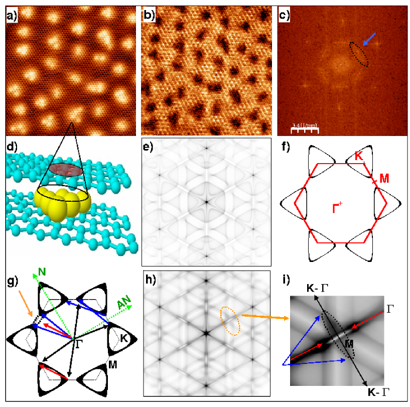
Figure 15: a) Topographic image taken at -1.4V ($13\times 13nm^{2}$) of ML graphene with the intercalated gold clusters underneath. b) Same region dI/dV map at +0.9V (unoccupied states). c) FT of b). e) and h) are the JDOS calculation of the CEC given in f) and g) respectively. i) is a zoom of the ellipitic feature encircled in h). Blue and red arrows correspond to the momentum vectors associated to the black vectors. The expected features in the JDOS calculation that are not observed experimentally are associated to momentum symbolized by red arrows.

V General conclusion

We have shown that simple JDOS calculations and their comparison with the FT-STS maps provide an accurate determination of the size and shape of circular, and even non-circular free electron-like constant energy contours. These contours in turn provide precise information about the quasiparticle dispersion, and fine details about fairly complex 2D band structures. On the other hand, we have shown that the T-matrix approximation becomes absolutely necessary for more complex systems where more than one quantum number is involved in the scattering process.

While in order to apply the T-matrix approximation one needs to have the exact form of the tight-binding Hamiltonian of a system, the JDOS approach does not rely on the exact form of the Hamiltonian, but on the phenomenological form of the equal energy contours. Its advantage is that it can be used even if the Hamiltonian of a system is not known, but the equal energy contours are known from a different experiment such as ARPES; this allows one to have an intuitive reading of the FT features. The results of the T-matrix and the JDOS approximations are in general the same for a symmetrical, quadratic-dispersing system; for example, for the case of Au(111), while not shown here, both the T-matrix and the JDOS approximations yield circles of high intensity in the FT-STS spectra. However, for more complicated systems, these two methods may yield different results, and one notes that when the features predicted by JDOS are not observed experimentally, as it is the case of graphene, the physics of the system is in general more complicated, and a full T-matrix calculation is needed to describe it.

We notice that in general a good agreement with angle resolved photoemission data has been found and this indicates that both methods (ARPES and FT-STS) probe the same quasiparticle excitations of the system. This technique provides the possibility to measure the band dispersion modification generated by specific defects of different nature. This allows to test locally the effect of specific modifications and functionalization of well-known surfaces which is not possible with ARPES measurements which requires to prepare large homogeneous surface in order to obtain reliable data.

- (1) M.F. Crommie, C.P. Lutz, and D.M. Eigler, Science 262, 218 (1993).
- (2) E.J. Heller, M.F. Crommie, C.P. Lutz, and D.M. Eigler Nature 369, 464 (1994).
- (3) M.F. Crommie, C.P. Lutz, D.M. Eigler, and E.J. Heller, Surf. Rev. Lett. 2, 127 (1995).
- (4) H.C. Manoharan, C.P. Lutz, and D.M. Eigler, Nature bf 403, 512 (2000).
- (5) J. Friedel, Nuevo Cimento 7, 287 (1958).
- (6) M.A. Ruderman, and C. Kittel, Phys. Rev. 96, 99 (1954).
- (7) K. Yosida, Phys. Rev. 106, 893 (1957).
- (8) T. Kasuya, Prog. Theor. Phys. 16,45 (1956).
- (9) N. Knorr, H. Brune, M. Epple, A. Hirstein, M.A. Schneider, and K. Kern, Phys. Rev. B 65, 115420 (2002).
- (10) F. Gautier, and P. Lenglart, Phys. Rev. 139, A705 (1965).
- (11) F. Petroff, A. Barthélemy, D.H. Mosca, D.K. Lottis, A. Fert, P.A. Schroeder, W.P. Pratt Jr, R. Loloee, and S. Lequien, Phys. Rev. B 44, 5355 (1991).
- (12) P. Bruno, and C. Chappert, Phys. Rev. Lett. 67, 1602 (1991).
- (13) Y. Hasegawa, and Ph. Avouris, Phys. Rev. Lett. 71, 1071 (1993).
- (14) M.F. Crommie, C.P. Lutz, and D.M. Eigler, Nature 363, 524 (1993).
- (15) O. Jeandupeux, L. Bürgi, A. Hirstein, H. Brune, and K. Kern, Phys. Rev. B 59, 15926 (1999).
- (16) L. Bürgi, H. Brune, and K. Kern, Phys. Rev. Lett. 89, 176801 (2002).
- (17) M. Pivetta, F. Silly, F. Patthey, J.P. Pelz, and W.-D. Schneider, Phys. Rev. B 67, 193402 (2003).
- (18) P.T. Sprunger, L. Petersen, E.W. Plummer, E. Lægsgaard, and F. Besenbacher, Science 275, 1764 (1997).
- (19) L. Petersen, Ph. Hofmann, E.W. Plummer, and F. Besenbacher, J. of. Elec. Spec. and Rel. Mat. 109, 97 (2000).
- (20) Ph. Hoffmann, B.G. Brinner, M. Doering, H.P. Rust, E.W. Plummer, and A.M. Bradshaw, Phys. Rev. Lett. 79, 265 (1997).
- (21) J.E. Hoffman, K. McElroy, D.H. Lee, K.M. Lang, H. Eisaki, S. Uchida, and J.C. Davis, Science 297, 1148 (2002).
- (22) K. McElroy, R.W. Simmonds, J.E. Hoffman, D.H. Lee, J. Orenstein, H. Elsaki, S. Uchida, and J.C. Davis, Nature 422, 592 (2003).
- (23) M. Vershinin, S. Misra, S. Ono, Y. Abe, Y. Ando, and A. Yazdani, Science 303, 1995 (2004).
- (24) J.I. Pascual, G. Bihlmayer, Y.M. Koroteev, H.P. Rust, G. Ceballos, M. Hansmann, K. Horn, E.V. Chulkov, S. Blügel, P.M. Echenique, and Ph. Hofmann, Phys. Rev. Lett. 93, 196802 (2004).
- (25) F. Vonau, D. Aubel, G. Gewinner, C. Pirri, J.C. Peruchetti, D. Bolmont, and L. Simon, Phys. Rev. B 69, 081305(R) (2004).
- (26) F. Vonau, D. Aubel, G. Gewinner, J.C. Peruchetti, D. Bolmont, and L. Simon, Phys. Rev. Lett. 95, 176803 (2005).
- (27) L. Simon, F. Vonau, and D. Aubel, J. Phys. Cond. Matter 19, 355009 (2007).
- (28) L.M. Roth, H.J. Zeiger, and T.A. Kaplan, Phys. Rev. 16, 149 (1966).
- (29) A.J. van Bommel, J.E. Crombeen,and A. van Tooren, Surf.Sci. 48, 463 (1975).
- (30) I. Forbeaux, J.M. Themlin, and J.M. Debever, Phys. Rev. B 58, 16396 (1998).
- (31) L. Simon, J.L. Bischoff, and L. Kubler, Phys. Rev. B 60, 11653 (1999).
- (32) C. Berger, Z. Song, T. Li, X. Li, A.Y. Ogbazghi, R. Feng, Z. Dai, A.N. Marchenkov, E.H. Conrad, P.N. First, and W.A. de Heer, J. Phys. Chem. 108, 19912 (2004).
- (33) P. Lauffer, K.V. Emtsev, R. Graupner, Th. Seyller, L. Ley, S.A. Reshanov, and H.B. Weber, Phys. Rev. B 77, 155426 (2008).
- (34) T. Ohta, A. Bostwick, Th. Seyller, K. Horn, and E. Rotenberg, Science 313, 951 (2006).
- (35) C. Berger. Z. Song, X. Li, X. Wu, N. Brown, C. Naud, D. Mayou, T.Li, J. Hass, A.N. Marchenkov, E.H. Conrad, P.N. First, and W.A. de Heer, Science 312, 1191(2006).
- (36) B. Premlal, M. Cranney, F. Vonau, D. Aubel, D. Casterman, M.M. De Souza, and L. Simon, Appl. Phys. Lett. 94, 263115 (2009).
- (37) N.W. Ashcroft, and N. David Mermin, Solid State Physics, HRW international edition (1987), chapt. 17.
- (38) J.M. Ziman,Principles of the Theory of Solids second edition, Cambridge University Press
- (39) L. Stauffer, A. Mharchi, C. Pirri, P. Wetzel, D. Bolmont, G. Gewinner, and C. Minot, Phys. Rev. B 47, 10555 (1993).
- (40) P. Wetzel, C. Pirri, P. Paki, J.C. Peruchetti, D. Bolmont, and G. Gewinner, Solid. State. Com. 82, 235 (1992).
- (41) M.H. Tuilier, P. Wetzel, C. Pirri, D. Bolmont, and G. Gewinner, Phys. Rev. B 50, 2333 (1994).
- (42) A. Blandin, Thesis, University of Paris-Sud, Orsay (1961).
- (43) C. Rogero, C. Koitzsch, M.E. Gonzalez, P. Aebi, J. Cerda, and J.A. Martin-Gago, Phys. Rev. B 69, 045312 (2004).
- (44) R.S. Markiewicz, Phys. Rev. B 69, 214517 (2004).
- (45) K. McElroy, G.H. Gweon, S.Y. Zhou, J. Graf, S. Uchida, H. Eisaki, H. Takagi, T. Sasagawa, D.H. Lee, and A. Lanzara, Phys. Rev. Lett. 96, 067005 (2006).
- (46) Q.H. Wang, and D.H. Lee, Phys. Rev. B 67, 02511(R) (2003).
- (47) L. Capriotti, D.J. Scalapino, and R.D. Sedgewick, Phys. Rev. B 68, 014508 (2003).
- (48) O. Kodra, and W.A. Atkinson, Phys. Rev. B 73, 045404 (2006).
- (49) G.F. Sun, Y. Liu, Y. Qi, J.F. Jia, Q.K. Xue, M. Weinert, and L. Li, Nanotech. 21, 435401(2010).
- (50) G. Mahan, Many-Particle Physics, Kluwer Academics/Plenum Publishers, New York, ISBN 0-306-46338-5 (2000), chapt. 4.
- (51) H. Bruus, and K. Flensberg, Many-Body Quantum Theory in Condensed Matter Physics - An Introduction, Oxford University Press, Oxford, ISBN 0 19 856633 6 (2005), chapt. 5, etc.
- (52) J.M. Byers, M.E. Flatté, and D.J. Scalapino, Phys. Rev. Lett. 71, 3363 (1993).
- (53) M.I. Salkola, A.V. Balatsky, and D.J. Scalapino, Phys. Rev. Lett. 77, 1841 (1996).
- (54) W. Ziegler, D. Poilblanc, R. Preuss, W. Hanke, and D.J. Scalapino, Phys. Rev. B 53, 8704 (1996).
- (55) P.J. Hirschfeld, P. Wölfle, and D. Einzel, Phys. Rev. B 37, 83 (1988).
- (56) A. Polkovnikov, S. Sachdev, and M. Vojta, Phys. Rev. Lett. 86, 296 (2001).
- (57) D. Podolsky, E. Demler, K. Damle, and B.I. Halperin, Phys. Rev. B 67, 094514 (2003).
- (58) Q.H. Wang, and D.H. Lee, Phys. Rev. B 67, 020511 (2003).
- (59) C. Bena, S. Chakravarty, J. Hu, and C. Nayak, Phys. Rev. B 63, 134517 (2004).
- (60) C. Bena, and S. Kivelson, Phys. Rev. B 72, 125432 (2005).
- (61) C.Bena, Phys. Rev. Lett. 100, 076601 (2008).
- (62) T.O. Wehling, A.V. Balatsky, M.I. Katsnelson, A.I. Lichtenstein, K. Scharnberg, and R. Wiesendanger, Phys. Rev. B 75, 125425 (2007).
- (63) N.M.R. Peres, F.D. Klironomos, S.W. Tsai, J.R. Santos, J.M.B. Lopes dos Santos, and A.H. Castro Neto, Europhys. Lett. 80, 67007 (2007).
- (64) N.M. Peres, F. Guinea, and A.H. Castro Neto, Phys. Rev. B 73, 125411 (2006).
- (65) M.A.H. Vozmediano, M.P. López-Sancho, T. Stauber, and F. Guinea, Phys. Rev. B 72, 155121 (2005).
- (66) T. Ando, J. Phys. Soc. Jpn. 75, 074716 (2006).
- (67) Y. G. Pogorelov, arXiv:condmat/0603327.
- (68) Y.V. Skrypnyk, and V.M. Loktev, Phys. Rev. B 73, 241402(R) (2006).
- (69) Y.V. Skrypnyk, and V.M. Loktev, Phys. Rev. B 75, 245401 (2007).
- (70) M.I. Katsnelson, and A.K. Geim, Phil. Trans. R. Soc. A 366, 195 (2008).
- (71) A.H. Castro Neto, and F. Guinea, Phys. Rev. Lett. 103, 026804 (2009).
- (72) P. Ruffieux, M. Melle-Franco, O. Gröning, M. Bielmann, F. Zerbetto, and P. Gröning, Phys. Rev. B 71, 153403 (2005).
- (73) P. Ruffieux, O. Gröning, P. Schwaller, L. Schlapbach, and P. Gröning, Phys. Rev. Lett. 84, 4910 (2000).
- (74) H. Yang, A.J. Mayne, M. Boucherit, G. Comtet, G. Dujardin, and Y. Kuk, Nanoletters 10, 943 (2010).
- (75) P.R. Wallace, Phys. Rev. 71, 622 (1947).
- (76) P. van Mieghem, Rev. Mod. Phys 64, 755 (1992).
- (77) E. McCann, Phys. Rev. B 74, 245426 (2006).
- (78) E. McCann, and V.I. Fal’ko, Phys. Rev. Lett. 96, 086805 (2006).
- (79) J. Nilsson, A.H. Castro Neto, N.M.R. Peres, and F. Guinea, Phys. Rev. B 73, 214418 (2006).
- (80) S.A. Kivelson, I.P. Bindloss, E. Fradkin, V. Oganesyan, J.M. Tranquada, A. Kapitulnik, and C. Howald, Rev. Mod. Phys. 75, 1201 (2003).
- (81) V.V. Cheianov, and V.I. Fal’ko, Phys. Rev. Lett. 97, 226801 (2006).
- (82) E.Mariani, L.I. Glazman, A. Kamenev, and F. von Oppen, Phys. Rev. B 76, 165402 (2007).
- (83) A.K. Geim, and K.S. Novoselov, Nature Mater. 6, 183 (2007).
- (84) M.I. Katsnelson, K.S. Novoselov, and A.K. Geim, Nature Phys. 2, 620 (2006).
- (85) T. Ando, T. Nakanishi, and R. Saito, J. Phys. Soc. Jpn. 67, 2857 (1998).
- (86) M.I. Katsnelson, and K.S. Novoselov, Solid State Commun. 143, 3 (2007).
- (87) M.I. Katsnelson, Phys. Rev. B 76, 073411 (2007).
- (88) P. Mallet, F. Varchon, C. Naud, L. Magaud, C. Berger, and J.Y. Veuillen, Phys. Rev. B 76, 041403(R)(2007).
- (89) G.M. Rutter, J.N. Crain, N.P. Guisinger, T. Li, P.N. First, and J.A. Stroscio, Science 317, 219 (2007).
- (90) I. Brihuega, P. Mallet, C. Bena, S. Bose, C. Michaelis, L. Vitali, F. Varchon, L. Magaud, K. Kern, and J.Y. Veuillen, Phys. Rev. Lett. 101, 206802 (2008).
- (91) L. Simon, C. Bena, F. Vonau, D. Aubel, H. Nasrallah, M. Habar and J.C. Peruchetti, Eur. Phys . J. B, 69, 355 (2009).
- (92) M. Cranney, F. Vonau, P.B. Pillai, E. Denys, D. Aubel, M.M. De Souza, C. Bena, and L. Simon, Euro. Phys. Lett. 91, 66004 (2010).
- (93) A. Bostwick, T. Ohta, T. Seyller, K. Horn, and E. Rotenberg, Nature Phys. 3, 36 (2007).
- (94) S.Y. Zhou, G.H. Gweon, A.V. Fedorov, P.N. First, W.A. de Heer, D.H. Lee, F. Guinea, A. H. Castro Neto, and A. Lanzara, Nature Mater. 6, 770 (2007).
- (95) K. McElroy, J. Lee, J.A. Slezak, D.H. Lee, H. Eisaki, S. Uchida, and J.C. Davis, Science 309, 1048 (2005).
- (96) A. Fang, C. Howald, N. Kaneko, M. Greven, and A. Kapitulnik, Phys. Rev. B 70, 214514 (2004).
- (97) V.W. Brar, Y. Zhang, Y. Yayon, and T. Ohta, Appl. Phys. Lett. 91, 122102 (2007).
- (98) Y. Zhang, V.W. Brar, F. Wang, C. Girit, Y. Yayon, M. Panlasigui, A. Zettl, and M.F. Crommie, Nature Phys. 4, 627 (2008).
- (99) C. Bena, Phys. Rev. B 79, 125427 (2009).
- (100) E. Cockayne, G.M. Rutter, N.P. Guisinger, J.N. Crain, P.N. First, and J.A. Stroscio, arXiv:1008.3574.
- (101) in preparation
- (102) C. Bena, and L. Simon, Phys. Rev B 83, 115404 (2011).