Femtosecond pulses in a dense two-level medium: Spectral transformations, transient processes, and collisional dynamics

Abstract

Propagation of ultrashort optical pulses in a dense resonant medium is considered in the semiclassical limit. In our analysis, we place emphasis on several main points. First, we study transformations of spectra in the process of pulse propagation and interactions with another pulse. The second point involves the transient processes (including pulse compression) connected with self-induced transparency soliton formation inside the medium. Finally, the third aspect is the study of collisions of co- and counter-propagating pulses in the medium. In the last case, the investigation of symmetric and asymmetric collisions shows the possibility of effectively controlling the parameters of transmitted radiation.

I Introduction

A two-level medium, i.e. a medium composed of a collection of two-level systems (atoms, molecules, etc.), is the basic quantum-mechanical model in the theory of light-matter interaction. It plays the same fundamental role as a harmonic oscillator in classical physics. Therefore, the comprehensive study of this model and its generalizations is one of the most important problems in theoretical optics. The two-level model has allowed the description of a number of well-known effects Allen ; Kryukov including the effect of self-induced transparency McCall ; Poluektov . Among the further generalizations of the model we single out the one which takes into account the near dipole-dipole interactions between the elements of the dense medium due to introduction into the equations of the so-called local-field correction Bowd93 ; Cren08 . In stationary regime, the presence of the local field results in the remarkable effect of intrinsic optical bistability Hopf ; Ben-Aryeh ; Friedberg ; Hehlen .

In the regime of optical pulses, the investigation of local-field effects is linked with solitonic dynamics Bowd91 ; Afan02 , optical switching Cren92 ; Scalora , etc. It was shown Scalora that, in the dense two-level medium, the scale of population and field changes becomes so short that one cannot use the common slowly varying envelope approximation in space (SVEAS) to describe light pulse propagation. Therefore, one should use the full (not truncated) Maxwell wave equation. This is the case in the present paper where we consider one-dimensional problem of ultrashort (femtosecond) light pulse propagation in a two-level medium. Two remarks should be made here. First, as discussed in our previous work Novit1 , the local-field effects depend strongly on the duration of the pulse. For the femtosecond pulses considered in this paper, these effects are negligible. However, the dynamics of the pulse cannot be fully described by the usual self-induced transparency (SIT) model. This fact leads us to the second remark. In the dense two-level medium, calculations using the wave equation without SVEAS show the slow attenuation of SIT solitons as was predicted in Ref. Novit . This and similar other effects provide the rich dynamics of transient processes which are one of the main objects of this investigation.

Another aim of our research is to study in detail the complex dynamics of pulse collisions in the two-level medium. Interaction of counter-propagating solitons was previously a research issue in both the cases of two-level Afan ; Shaw and three-level media Pusch ; Park ; Loiko . In the appropriate section, we will return to some of this works and discuss the further progress achieved in this paper. Here, it is worth noting that we try to trace step-by-step the changes in parameters of the pulses obtained at relatively short distances due to the high density of the medium. In addition, collisions of solitons and attendant effects were theoretically and experimentally studied in different other systems such as optical fibers Malomed , photorefractive crystals Krolik1 ; Krolik2 , and photonic crystals Petrovic ; Erkintalo . In this paper we consider temporal solitons, while the collisions between spatial ones were reported as well Cohen ; Petrovic .

The structure of the paper corresponds to the gradual transition from the relatively simple situations to the more complicated ones. Section II is devoted to the case of single pulse propagation in a dense two-level medium paying attention to the transformations of light spectrum as it moves through the medium. In Section III we consider interaction of co-propagating solitons, especially those overtaking one another. Section IV is dedicated to the case of counter-propagating pulses colliding in the medium. In particular, we analyze the situation of the so-called symmetric collision there. Finally, in Section V we study the asymmetric collisions between the counter-propagating solitons.

II Single pulse propagation

We start with the semiclassical Maxwell-Bloch system for population difference $W$, microscopic polarization $R$, and electric field amplitude $\Omega^{\prime}=\Omega/\omega=(\mu/\hbar\omega)E$ (i.e. normalized Rabi frequency) Bowd93 ; Cren96 ,

$$\frac{dR}{d\tau} = i\Omega^{\prime}W+iR(\delta+\epsilon W)-\gamma_{2}R,$$ (1)

$$\frac{dW}{d\tau} = 2i(\Omega^{\prime*}R-R^{*}\Omega^{\prime})-\gamma_{1}(W-1),$$ (2)

$$\frac{\partial^{2}\Omega^{\prime}}{\partial\xi^{2}} - \frac{\partial^{2}\Omega^{\prime}}{\partial\tau^{2}}+2i\frac{\partial\Omega^{\prime}}{\partial\xi}+2i\frac{\partial\Omega^{\prime}}{\partial\tau}$$ (3)

$$=3\epsilon\left(\frac{\partial^{2}R}{\partial\tau^{2}}-2i\frac{\partial R}{\partial\tau}-R\right),$$

where $\tau=\omega t$ and $\xi=kz$ are dimensionless arguments; $\delta=\Delta\omega/\omega$ is the normalized detuning of the field carrier (central) frequency $\omega$ from atomic resonance; $\gamma_{1}=(\omega T_{1})^{-1}$ and $\gamma_{2}=(\omega T_{2})^{-1}$ are the rates of longitudinal and transverse relaxation, respectively; $k=\omega/c$ is the wavenumber, and $c$ is the light speed in vacuum; $\epsilon=\omega_{L}/\omega=4\pi\mu^{2}C/3\hbar\omega$ is the normalized Lorentz frequency. Here we assume that the background dielectric permittivity of the medium is unity (two-level atoms in vacuum). Note that in Eq. (3) we do not use slowly-varying envelope approximation (SVEA) which cannot hold true even for thin films of the medium Scalora .

In this paper we consider propagation of ultrashort pulses with Gaussian shape $\Omega=\Omega_{p}\exp(-t^{2}/2t_{p}^{2})$ where $t_{p}$ is the pulse duration. Amplitude of pulses is measured in the units of the characteristic Rabi frequency $\Omega_{0}=\sqrt{2\pi}/2t_{p}$, which corresponds to the so-called $2\pi$-pulse Novit . For calculations the values $T_{1}=1$ ns and $T_{2}=0.1$ ns are taken, so that femtosecond pulses appear to be in the regime of coherent interaction with the resonant medium. The spectra of pulses plotted in this paper are obtained as the absolute values of the Fourier transform of the corresponding field profiles. The spectra are normalized on the peak value of the incident pulse spectrum which is recognized as the unity. We use the following parameters of calculations which hold true throughout the paper if the other is not stated: $n_{d}=1$, $\omega_{L}=10^{11}$ s^-1, $\delta=0$, $\lambda=0.5$ $\mu$m, $t_{p}=50$ fs.

In Fig. 1 we demonstrate the results of propagation simulation for the pulse with high peak amplitude ($\Omega_{p}=1.5\Omega_{0}$). As it was shown in Ref. Novit , an ultrashort pulse in dense resonant medium experiences compression. The reason for this is perhaps the effect of self-phase modulation reported in Ref. Scalora . The effect of compression is characterized by a certain distance of optimal compression: After this distance the pulse slowly attenuates due to dispersion. For the layer of approximately optimal thickness, the main part of the pulse is transmitted and compressed, while some part of its energy is absorbed and then reemitted [Fig. 1(a)]. The spectrum of the main part has the typical bell shape, while the reemitted light has a dip at the resonant wavelength [Fig. 1(d)]. This can be connected with effective reabsorption of low-intensity light at the resonant frequency. At the same time the main, high-intensity part of the pulse is almost not absorbed due to the self-induced transparency (SIT) mechanism. The resulting spectrum of the transmitted radiation is shown in Fig. 1(b): The two peaks are situated at both sides of the central wavelength. The low-level reflected light has a dip in its spectrum as well [Fig. 1(c)].

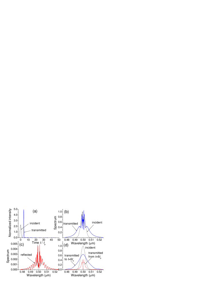
Figure 1: (Color online) (a) Intensity profile of the pulse transmitted through the layer of thickness $L=100\lambda$. (b) and (c) Spectra of transmitted and reflected light respectively. The spectra were calculated for the radiation appeared in the time interval from $t=-3t_{p}$ (start of the incident pulse) to $t=100t_{p}$. (d) Spectra of transmitted light calculated for the radiation appeared in the other time intervals (from $t=-3t_{p}$ to $t=6t_{p}$, and from $t=6t_{p}$ to $t=100t_{p}$). The amplitude of the pulse $\Omega_{p}=1.5\Omega_{0}$. The local-field correction is not taken into account.

Figure 2: (a) and (b) Spectra of transmitted light in the cases of absence and presence of local-field correction, respectively. The spectra were calculated for the radiation appeared in the time interval from $t=-3t_{p}$ (start of the incident pulse) to $t=100t_{p}$. (c) Difference between the spectra shown in plots (a) and (b). (d) Difference between intensity profiles of transmitted light in the cases of absence and presence of local-field correction, respectively. The amplitude of the pulse $\Omega_{p}=1.5\Omega_{0}$.

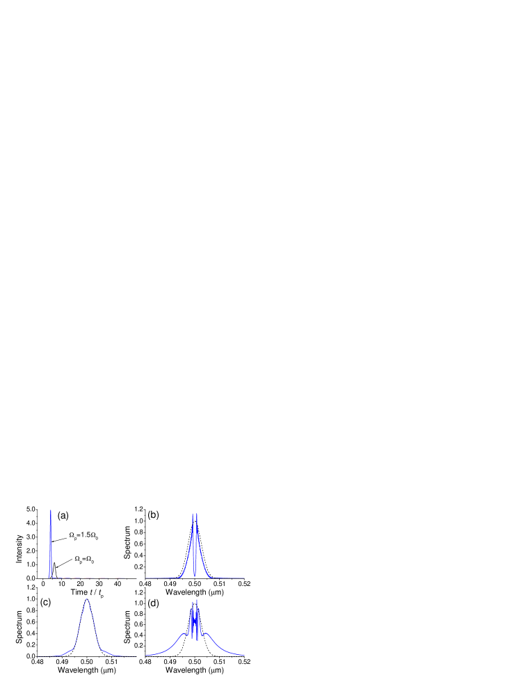
Figure 3: (Color online) (a) Intensity profiles of the light transmitted through the layer of thickness $L=100\lambda$ for the pulses with different peak amplitudes. (b), (c), (d) Spectra of transmitted light for the pulses with different peak amplitudes ($\Omega_{p}=0.5\Omega_{0}$, $\Omega_{0}$ and $1.5\Omega_{0}$, respectively). The spectra were calculated for the radiation appeared in the time interval from $t=-3t_{p}$ (start of the incident pulse) to $t=100t_{p}$. The dashed line corresponds to the spectrum of incident pulse. The local-field correction is taken into account.

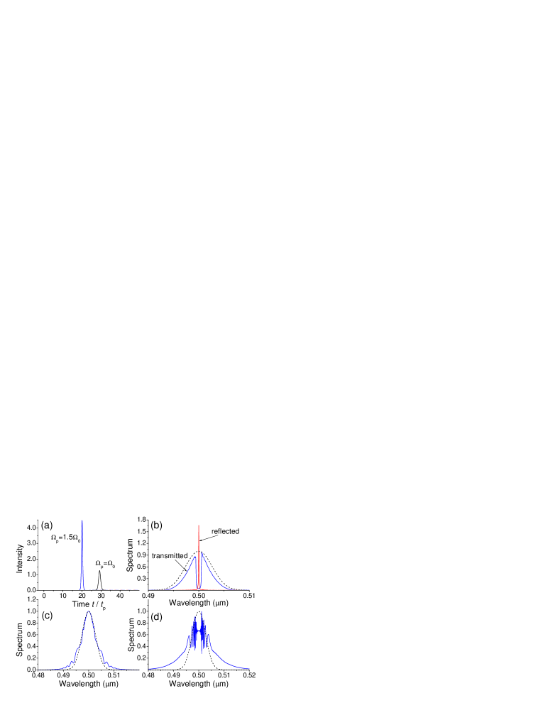
Figure 4: (Color online) (a) Intensity profiles of the light transmitted through the layer of thickness $L=500\lambda$ for the pulses with different peak amplitudes. (b) Spectra of transmitted and reflected light for the pulse with the peak amplitude $\Omega_{p}=0.5\Omega_{0}$. (c), (d) Spectra of transmitted light for the pulses with the peak amplitudes $\Omega_{p}=\Omega_{0}$ and $1.5\Omega_{0}$, respectively. The spectra were calculated for the radiation appeared in the time interval from $t=-3t_{p}$ (start of the incident pulse) to (c), (d) $t=200t_{p}$, (b) $t=600t_{p}$. The dashed line corresponds to the spectrum of incident pulse.

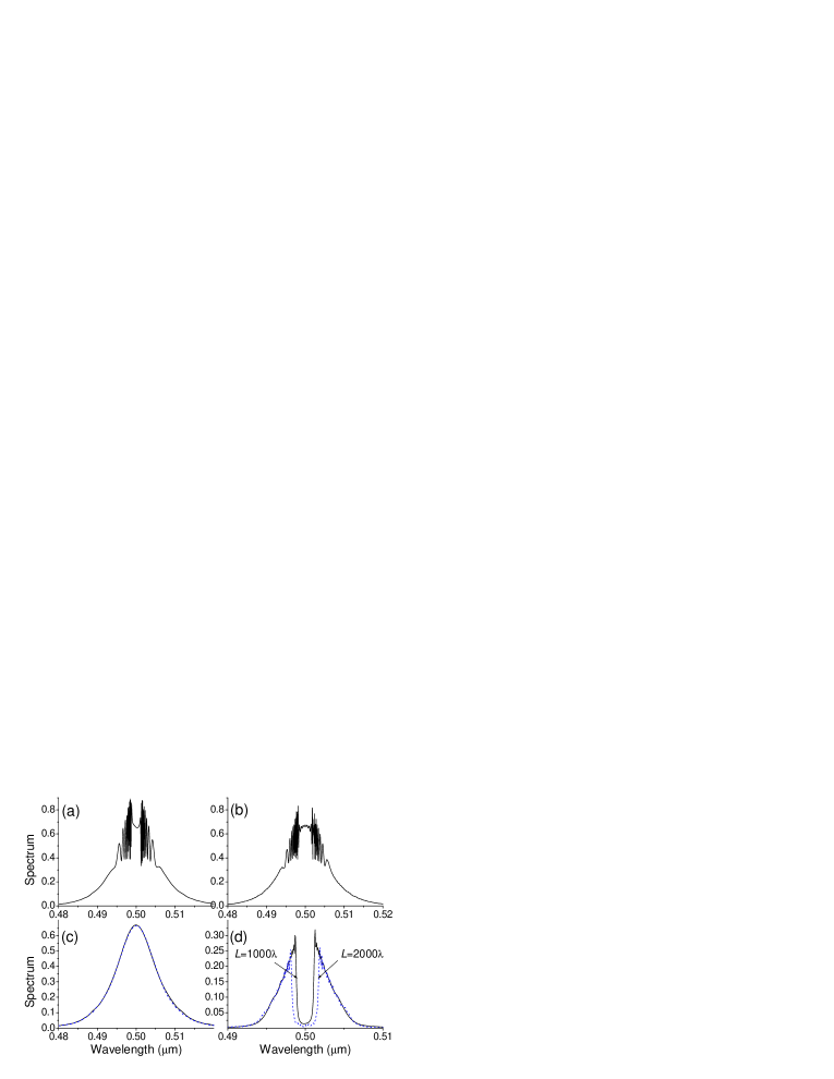
Figure 5: (Color online) Spectra of transmitted light for the pulse with the initial peak amplitude $\Omega_{p}=1.5\Omega_{0}$ after propagation of (a) $L=1000\lambda$, (b) $L=2000\lambda$. (c) Spectra of the main part of transmitted pulse and (d) spectra of the ”tail” for $L=1000\lambda$ and $2000\lambda$.

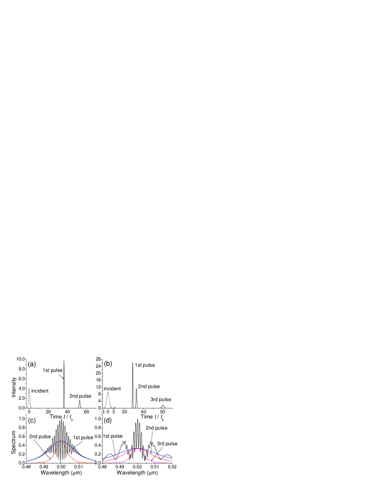
Figure 6: (Color online) (a), (b) Intensity profiles of the light transmitted through the layer of thickness $L=1000\lambda$ for the pulses with peak amplitudes $\Omega_{p}=2\Omega_{0}$ and $3\Omega_{0}$, respectively. (c), (d) Spectra of transmitted light corresponding to the upper figures.

Figure 1 was obtained in the absence of the local-field correction (LFC), that is without the term $\epsilon W$ in Eq. (1). To evaluate the influence of local field, we calculate the difference between the transmitted light spectra obtained with and without LFC [Fig. 2(c)]. It is seen that LFC leads to the significant change in spectrum (more than $8\%$ of the maximal value), while the intensity profile remains almost unchanged [Fig. 2(d)] in accordance with the results previously reported Novit1 . The difference between spectra is mainly due to the late, reemitted radiation which interacts with the medium for a time long enough to feel the local field. Nevertheless the overall form of the spectrum is the same as one can ascertain comparing Figs. 2(a) and (b). Therefore, hereinafter all the results are obtained taking into account LFC.

Returning to Fig. 1, we should once more emphasize the role of pulse ”tail” in formation of the fine structure of the complex spectrum of transmitted light. Note that the resulting spectrum is not a simple superposition of the two others [see Fig. 1(d)] because of interference term which should be taken into account here. Figure 3 shows the spectra for the transmitted pulses with different initial peak amplitude $\Omega_{p}$. The simplest case is observed for $\Omega_{p}=\Omega_{0}$, i.e. for the $2\pi$-pulse. Such a pulse is only slightly compressed and can propagate for a long distance almost without change. Its spectrum is generally coincident with that of the incident pulse [Fig. 3(c)]. The pulses with amplitudes larger and smaller than $\Omega_{0}$ demonstrate significant pulse transformations. Low-intensity pulse (in our case $\Omega_{p}=0.5\Omega_{0}$) experiences strong absorption on the central frequency, so that the output radiation has no any regular profile [it is not seen in Fig. 3(a) due to its proximity to zero]. The overall energy leaving the medium in this case is about half of the initial pulse energy (for the calculational conditions denoted in the caption of Fig. 3). This output energy is mainly concentrated in the side bands of the spectrum as seen in Fig. 3(b). In the case of high-intensity pulse ($\Omega_{p}=1.5\Omega_{0}$), absorption is not significant and almost all energy transmits through the medium. However, its spectrum [Fig. 3(d)] implies that some part of the radiation is transferred from the central wavelength to the side bands.

The next step is to consider the transformations of spectra with distance traveled by the pulses in the two-level medium (we increase the distance by the factor of $5$, i.e. to $L=500\lambda$). We find that the spectrum of $2\pi$-pulse gets more distorted as it propagates inside the medium for a longer distance [Fig. 4(c)]. In Fig. 4(b) one can see that the spectrum of low-intensity transmitted pulse has the same form as previously. In this figure the spectrum of reflected light is plotted as well. Reflected radiation is concentrated mainly very close to the central (resonant) frequency. In other words, the medium in this case can serve as a very-narrow-bandwidth filter. However, the efficiency of such a filter is not large because only a few percent of the incident light is reflected.

The case $\Omega_{p}=1.5\Omega_{0}$ is of maximal interest to us due to the strongly pronounced role of the pulse ”tail”. Comparison of Figs. 3(d) and 4(d) shows that the side bands move away from the resonant wavelength as the pulse propagates in the medium. This is also proved in Fig. 5(a) and (b). This transformation of spectrum is due to change in the spectrum of the ”tail”: The central dip gets wider [Fig. 5(d)]. Note that the main part of the pulse is characterized by the same spectrum [Fig. 5(c)]. It remains almost unchanged because the main part demonstrates invariant propagation in the regime of self-induced transparency (SIT-soliton). However, the main pulse very slowly attenuates though not so fast as was reported previously Novit . This is due to higher accuracy of our calculations in the current investigation.

If the pulse amplitude is high enough ($\Omega_{p}\geq 2\Omega_{0}$), the splitting of the pulse into several solitons can be observed. The examples of spectral transformations connected with this splitting are shown in Fig. 6. Comparison between the smooth spectra of separate solitons and the resulting jagged one implies that the phase relations between frequency components plays an important role. This interference is especially characteristic for the pulse splitting into three components ($\Omega_{p}=3\Omega_{0}$). In this case [Fig. 6(d)], apart from the central band, the spectrum has several pronounced and wide side bands. It is also worth noting that the first soliton has always the widest spectrum while every next one is more narrow. This corresponds to the fact that the first pulse is more compressed than any consecutive one.

III Co-propagating pulses

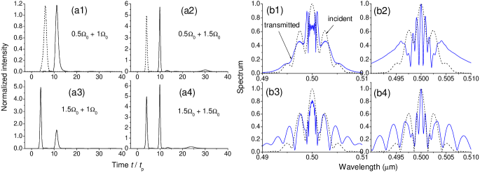
Figure 7: (Color online) (a) Intensity profiles and (b) spectra of the light transmitted through the layer of thickness $L=100\lambda$ for the pairs of incident pulses. The numbers at (a) and (b) correspond to different peak amplitudes of incident pairs: (1) $0.5\Omega_{0}+\Omega_{0}$, (2) $0.5\Omega_{0}+1.5\Omega_{0}$, (3) $1.5\Omega_{0}+\Omega_{0}$, (4) $1.5\Omega_{0}+1.5\Omega_{0}$. The time interval between the maxima of incident pulses is $6t_{p}$. The dotted line denotes (a) the transmitted single pulse with initial amplitude $\Omega_{0}$ (1) and $1.5\Omega_{0}$ (2); (b) the spectra of initial pair of pulses.

Figure 8: (a) Intensity profiles and (b) spectra of the light transmitted through the layers of different thicknesses. The calculations were performed for the pair of incident pulses $\Omega_{0}+1.5\Omega_{0}$. The time interval between the maxima of incident pulses is $6t_{p}$.

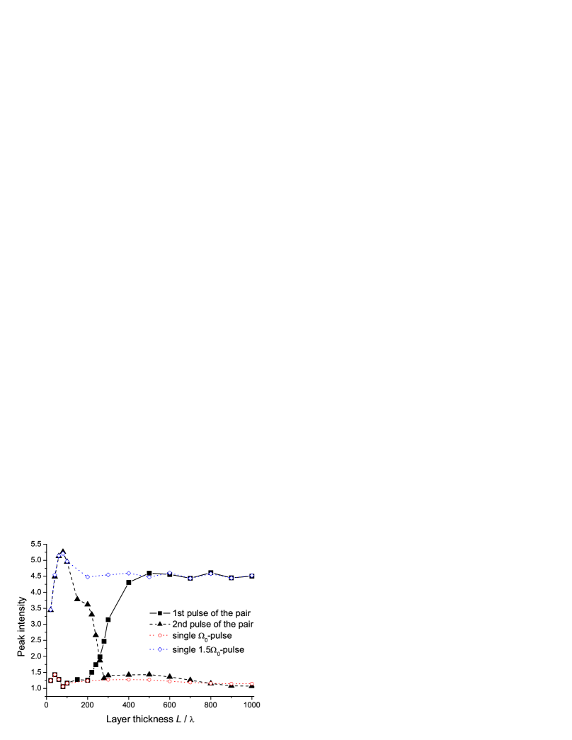
Figure 9: (Color online) Dependence of peak intensity of the light transmitted through the layer on its thickness. The calculations were performed for the pair of incident pulses $\Omega_{0}+1.5\Omega_{0}$ and for the single pulses $\Omega_{0}$ and $1.5\Omega_{0}$.

Figure 10: Intensity profiles of the light transmitted through the layers of different thicknesses; the reflected light has the identical envelope. The calculations were performed for the pair of counter-propagating incident pulses with amplitude $\Omega_{0}$.

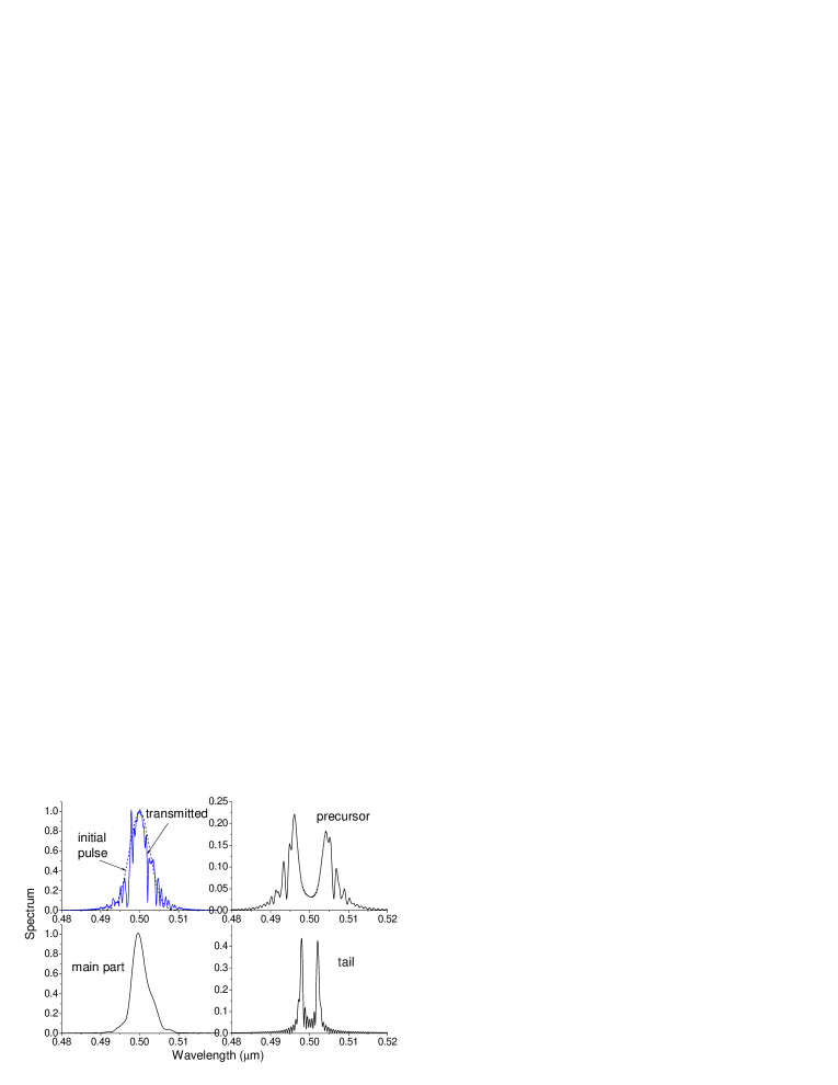
Figure 11: (Color online) Spectrum of light transmitted through the layer of thickness $L=1000\lambda$. The calculations were performed for the pair of counter-propagating incident pulses with amplitude $\Omega_{0}$.

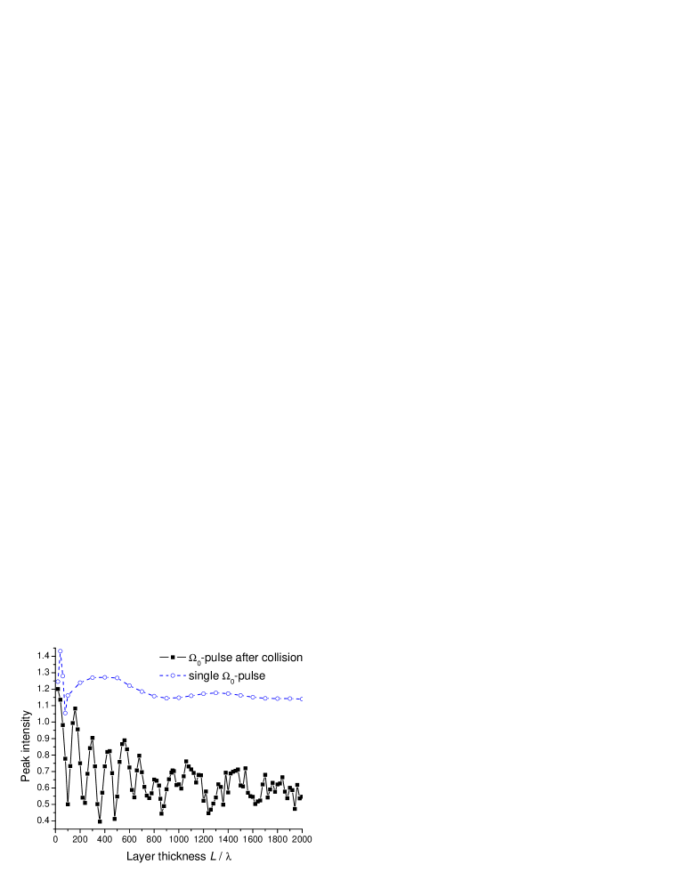
Figure 12: (Color online) Dependence of peak intensity of the light transmitted through the layer on its thickness. The calculations correspond to the case represented in Fig. 10.

Now let us consider the process of interaction between two pulses co-propagating in the dense two-level medium. Some preliminary results were published previously Novit . However, in this paper we present extended and more accurate calculational results. First, in Fig. 7(a) we show how the intensity of the second pulse changes under the influence of the first one. The time interval between the peaks of two incident co-propagating pulses is taken to be $6t_{p}$. It is seen that the first pulse loosing part of its energy causes some increase in the intensity of the second one in comparison with the case of the single pulse (this corresponds to the dotted lines). This is especially evident in the case of Fig. 7(a4). Figures 7(b) demonstrate the transformations of spectra due to simultaneous compression and interactions between the pulses. Note that the spectrum of the pair $0.5\Omega_{0}+1\Omega_{0}$ [Fig. 7(b1)] is similar to the spectrum of the single pulse with amplitude $1.5\Omega_{0}$ [Fig. 4(d)] and can be treated as composed from the spectra of pulses with $0.5\Omega_{0}$ and $\Omega_{0}$ [Fig. 4(b) and (c)]. Other spectra are characterized by appearance of strong side lobes and complex fine structure in the central part as seen in Fig. 7(b2).

One particular case (the pair $1\Omega_{0}+1.5\Omega_{0}$) is worth considering in detail here. This is because the second pulse of this pair propagates in the medium faster than the first one as results from Fig. 4(a). This means that, though the $2\pi$-pulse does not influence the second pulse at short distances, their interaction should be getting stronger as they co-propagate in the medium. The reason for this distinction in pulse velocity can be easily understood on the basis of the well-known expression for the stationary pulse Poluektov ,

$$\frac{1}{u}=\frac{1}{c}+\frac{\alpha t_{p}}{2},$$ (4)

where $u$ is the group velocity of the pulse, $c$ is the vacuum light speed, $\alpha\sim Ct_{p}$ is the extinction coefficient, $C$ is the concentration of two-level atoms, $t_{p}$ is the stationary pulse duration. Here we are interested only in relative speed of both pulses, so one can write

$$\frac{c/u_{1}-1}{c/u_{2}-1}=\frac{C_{1}t_{p1}^{2}}{C_{2}t_{p2}^{2}},$$ (5)

or, taking into account that the peak intensity $I_{p}\sim 1/t_{p}^{2}$,

$$\frac{c/u_{1}-1}{c/u_{2}-1}=\frac{C_{1}}{C_{2}}\frac{I_{p2}}{I_{p1}}.$$ (6)

This condition is perfectly satisfied as seen in Fig. 4(a) (for the case $C_{1}=C_{2}$). The concentration dependence also holds true as demonstrated by our careful examinations. This fact can be treated as one more proof of validity of our calculational scheme.

Thus, we can study the process of collision of two pulses co-propagating with different velocities. This case is demonstrated in Fig. 8. It is seen that the second, more intensive pulse overtakes the first one and, finally, at the length approximately $L=250\lambda$ they form a single pulse. This is indicated by the dramatic simplification of the spectrum which retains only one, central lobe. As the distance increases, this single pulse disintegrates, and the intensive pulse leaves the other behind. This fact corresponds to significant increase in complexity of the spectrum. The results of Fig. 8 also show that the intensity of the single pulse after coalescence is intermediate between the intensities of the pulses before the collision. The change in the peak intensities of the pulses as they co-propagate in the medium is depicted in Fig. 9. It is interesting to compare them with the behavior of intensity of a single pulse. It is seen that, after some transient process, the peak intensity of the single pulse remains almost invariable. This corresponds to the regime of solitonic propagation with the envelope perfectly described by hyperbolic secant function (this means that $1.5\Omega_{0}$-pulse with initial area of $3\pi$ transforms into a common $2\pi$-soliton). However, the intensity of the pulse is not strictly constant, it slightly fluctuates; so we cannot talk about strict, mathematical solitons but rather about realistic, physical ones. In addition, the amplitude of these fluctuations tends to decrease with the propagation distance. However, at larger distances the pulse slowly attenuates. For example, the intensity of the pulse with initial amplitude $1.5\Omega_{0}$ drops from approximately $4.5\Omega_{0}^{2}$ (at $L=1000\lambda$) to $3.75\Omega_{0}^{2}$ (at $L=10000\lambda$).

Figure 13: Distribution of (a) population difference and (b) light intensity inside the layer $L=1000\lambda=500$ $\mu$m at different time points. The calculations were performed for the pair of counter-propagating incident pulses with amplitude $\Omega_{0}$.

The next question is connected with the nature of the transient process: At first, the pulse is strongly compressed (on the distance of about $100\lambda$), and only then its envelope transforms to the solitonic one (hyperbolic secant) which is connected with some decrease in the pulse intensity. The initial compression of the pulse is due to the self-phase modulation effect and is strongly dependent on the form of the incident pulse. This compression can be observed even for the pulses with initial envelope described by hyperbolic secant. It is known that, at the same area (say, $2\pi$), the sech-pulse is wider than the Gaussian one, so that if the soliton is formed from the initial pulse, it would obtain greater duration. But it is not the case: the soliton forms from the compressed pulse. This compression can be characterized by the length value, namely, the so-called distance of optimal compression.

Returning to the collision of two pulses, we see (Fig. 9) that they strongly influence one another, but, after the change of the propagation order, the distance between them increases and the solitons are restored. One can say, that this figure demonstrates the interaction between the already formed or just forming solitons which are collision resistant.

IV Counter-propagating pulses

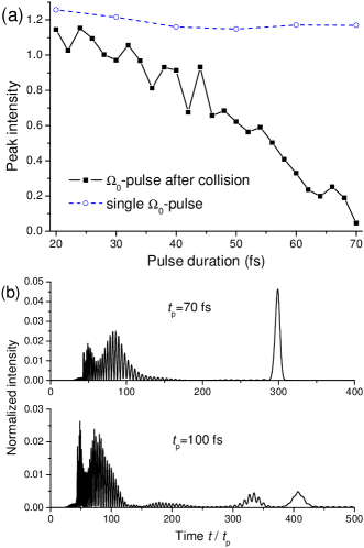
Figure 14: (Color online) (a) Dependence of peak intensity of the light transmitted through the layer on the duration of the initial $\Omega_{0}$-pulses. (b) Intensity of transmitted light for initial pulse durations $t_{p}=70$ fs and $t_{p}=100$ fs. The thickness of the layer is $L=1000\lambda$.

From the previous section we know that the collision of co-propagating pulses does not prevent formation of stationary pulses with the same characteristics as in the single pulse case. The collision of counter-propagating pulses has fundamentally different results. The reasons were studied previously in Refs. Afan ; Shaw . From mathematical point of view, two counter-propagating pulses cannot provide a stationary (solitonic) solution. Physically, this means that the absorption of some part of energy of the pulses occurs in the region of collision. Further we consider the dynamics of such collisions in detail.

We start from the collision of two Gaussian pulses with the amplitude $\Omega_{0}$ entering the medium at the same instant of time. In such symmetric geometry the light appearing from both ends of the layer (we can conditionally call it transmitted and reflected light) will be described by the same envelope. These envelopes are shown in Fig. 10 for different thicknesses of the layer. It is seen that the result of the collision strongly depends on the thickness $L$ and, as $L$ increases, the long precursor and tail become apparent (in Ref. Shaw only the tail was observed). The spectra of the precursor and the tail are similar (Fig. 11): they have a dip in the region of resonant wavelength, while radiation at this central frequency is strongly absorbed.

To study this thickness dependence of the collision, we simulate the process of interaction between the pulses in a wide range of thicknesses $L$. The results of these calculations for the peak intensity of the transmitted pulse are demonstrated in Fig. 12. It is seen that at relatively small length there are pronounced features which have a structure of something like resonances. For larger thicknesses the amplitudes of these resonances diminish, so that the peak intensity of the pulse tends to the approximately constant value. This implies that the resonances observed are connected with some transient process. This process can be traced using distribution of population difference and light intensity inside the medium at different instants of time (Fig. 13). The thickness of the layer ($L=1000\lambda$) is large enough for $2\pi$-solitons to be formed by the time of collision. This stationary pulse is characterized by the typical population difference profile (drop to full inversion and following rise to the ground state). One can easily ascertain that, at the location of collision, a strong absorption really occurs, so that some part of light energy remains inside the medium even after the pulses have gone away from each other. However, after collision, pulse propagation is not simple: After reaching minimum at $t=32t_{p}$, the pulse intensity grows ($t=34t_{p}$), then goes down again ($t=36t_{p}$), and so on. This process is obviously connected with fluctuations depicted in Fig. 9 and results in precursor and tail formation. It is reasonable to suggest that the resonances of Fig. 12 are due to pulse exiting in different moments of this transient process. But if the thickness of the layer is large, these fluctuations become smaller and smaller, so that at the output we have almost stationary pulse with the area $2\pi$ again and somewhat decreased intensity ($t=65t_{p}$).

The next important feature of pulse collisions is their dependence on the duration (or, equivalently, peak intensity) of the initial pulses. This dependence is shown in Fig. 14(a) and is in accordance with the results of Ref. Afan : For short and high-intensity $\Omega_{0}$-pulses, the influence of collision on pulse propagation is not significant. On the contrary, long and low-intensity pulses strongly interact with each other and, if the duration is large enough, the main pulse (soliton) disappears leaving only a precursor and a tail [see Fig. 14(b) for the pulses with $t_{p}=100$ fs]. Note that the area of the main pulse ($2\pi$) is conserved even in the case of dramatic decrease of its peak intensity. For example, the pulse corresponding to $t_{p}=70$ fs in Fig. 14(b) can be easily fitted by a hyperbolic secant function. This means that such low-intensity solitons undergo substantial broadening.

V Asymmetric collisions

Figure 15: (a) Dependence of peak intensity of the light transmitted through the layer on the incidence time difference between the two initial counter-propagating $\Omega_{0}$-pulses. (b) Corresponding behavior of propagation time calculated for the main pulse (soliton). The thickness of the layer is $L=1000\lambda$.

Figure 16: (a) Dependence of peak intensity of the light transmitted through the layer (for initial $\Omega_{0}$-pulse) on the amplitude of the counter-propagating pulse. (b) Corresponding behavior of propagation time calculated for the main pulse (soliton). The thickness of the layer is $L=1000\lambda$.

Figure 17: Distribution of (a) population difference and (b) light intensity inside the layer $L=1000\lambda$ at different time points. The calculations were performed for the pair of counter-propagating incident pulses: one with amplitude $\Omega_{0}$ and the other with $1.5\Omega_{0}$.

In previous section we considered the process of collision of the two identical counter-propagating pulses entering the medium at the same instant of time. Such geometry of the problem can be referred to as the symmetric one. Further we discuss the case of asymmetric collisions when the incidence time or intensity is different for both initial pulses.

Figure 15 shows the results of collision of the pulse with the amplitude $\Omega_{0}$ with the identical pulse which enters the medium at different time. Negative values of the incidence time difference $\Delta t$ means that the counter-propagating pulse is launched earlier than those propagating in the forward direction ($\Delta t=0$ corresponds to the symmetric situation considered in the previous section). In the case of $\Delta t<0$, the collision occurs closer to the input of the forward-propagating pulse, so that it has much time to form a stationary pulse after the collision. Therefore, the fluctuations of the peak intensity [Fig. 15(a)] are less pronounced in this case than for $\Delta t>0$. On both edges of this dependence (that is, for large absolute values of $\Delta t$) one obtains the trivial case of the single pulse propagation. The transition to this extreme regime has jump-like character on both sides of the peak intensity dependence. This symmetry does not take place for the time of pulse transmission through the layer [Fig. 15(b)]. For large negative $\Delta t$ the abrupt increase of time propagation occurs due to formation of the low-intensity (and, hence, slow) soliton near the very input. As the counter-propagating pulse enters the medium later and later, the fast initial pulse has enough time to pass a large fraction of distance before the collision happens. As a result, the propagation time decrease gradually as seen in Fig. 15(b). Thus, the collisional dynamics discussed imply the possibility of controlling such pulse parameters as its peak intensity and transmission time by proper choice of incidence time of the counter-propagating pulse.

Another approach to controlling the parameters of the transmitted pulse is to use the counter-propagating pulses of different intensities. In Fig. 16 one can see the change in peak intensity of $\Omega_{0}$-pulse as a function of the amplitude of the counter-propagating (controlling) one. As this amplitude grows, the peak intensity of the transmitted forward-propagating pulse decreases as well as its propagation velocity. Finally, in the region of amplitudes near $1.5\Omega_{0}$, the transmitted solitonic pulse is absent per se. We have only the precursor and the tail. For larger amplitudes of controlling pulse, the transmitted one appears again, of course, with larger retardation. However, collisional dynamics in this case are even more complex due to the effects of pulse splitting. Therefore, we will not consider the details of these multi-pulse interactions in the present investigation.

Instead, we turn to the case of complete soliton disappearance at the output of the medium when the amplitude of the controlling pulse equals $1.5\Omega_{0}$. The dynamics of level population difference and light intensity inside the medium depicted in Fig. 17 imply that the primary importance in this effect is likely to be connected with the residual excitation of the medium after passing the controlling pulse. Since its initial area is $3\pi$ (amplitude $1.5\Omega_{0}$), before the $2\pi$-soliton formes, some part of the energy is absorbed giving rise to the pronounced tail. It is seen that the collision leads to the significant loss of energy of the forward-propagating pulse while the controlling (high-intensity) pulse remains almost unchanged. Moving farther, the low-intensive pulse meets the tail of the counter-propagating one and the residual excitation and, finally, undergoes ultimate absorption in the medium. This absorbed energy gives fluorescent radiation in the long run as was stated in Ref. Shaw .

VI Conclusion

In this paper, we have considered the ultrashort (femtosecond) pulse interaction with a dense collection of two-level atoms. In other words, the light-medium interaction was investigated in the coherent regime when incoherent phenomenological relaxation can be neglected. Our study was conducted in semiclassical approximation, which is valid as we are not interested in the detailed description of the processes of spontaneous radiation Allen . In addition, semiclassical approach allows us to correctly take into account the local field correction Cren08 . Our calculations were performed for two-level atoms located in vacuum which corresponds to dense gaseous media. In order to consider solid-state systems (two-level atoms embedded in a dielectric, for example, quantum dots in semiconductor or glassy environment), one has to take into account the so-called local-field enhancement factor, as it was done in stationary regime Cren96a ; Novit2 . However, if the background dielectric is not absorptive, behavior of optical pulses reported in this paper is expected to be still valid for this more complex case (with the corresponding renormalization of the electric field).

In conclusion, we should discuss the prospects of pulse collision dynamics studied in the paper. Our accurate calculations show the self-healing effect for the co-propagating solitons but this is not the case for the counter-propagating pulses. Together with the transient processes of soliton formation, the strong interaction of the counter-propagating pulses provides for the rich dynamics of population difference and light intensity. The proper choice of the parameters of the colliding pulses allows one to effectively control the characteristics of light at the output of the medium. For example, one can obtain almost entire absorption of the soliton whose energy can be stored inside the medium, at least, for the relaxation time. The conditions of controlling pulse intensity by choosing the intensity or incidence time of the counter-propagating one can be considered as a basis of the peculiar logic gates or other elements for which the possibility of realization is still to be studied.

- (1) L. Allen and J.H. Eberly, Optical Resonance and Two-Level Atoms, (Wiley, New York, 1975).
- (2) P.G. Kryukov and V.S. Letokhov, Sov. Phys. Usp. 12, 641 (1970).
- (3) S.L. McCall and E.L. Hahn, Phys. Rev. 183, 457 (1969).
- (4) I.A. Poluektov, Yu.M. Popov, and V.S. Roitberg, Sov. Phys. Usp. 17, 673 (1975).
- (5) C.M. Bowden and J.P. Dowling, Phys. Rev. A47, 1247 (1993).
- (6) M. E. Crenshaw, Phys. Rev. A78, 053827 (2008).
- (7) F.A. Hopf, C.M. Bowden, and W.H. Louisell, Phys. Rev. A29, 2591 (1984).
- (8) Y. Ben-Aryeh, C.M. Bowden, and J.C. Englund, Phys. Rev. A34, 3917 (1986).
- (9) R. Friedberg, S.R. Hartmann, and J.T. Manassah, Phys. Rev. A40, 2446 (1989).
- (10) M.P. Hehlen, H.U. Güdel, Q. Shu, J. Rai, S. Rai, and S.C. Rand, Phys. Rev. Lett. 73, 1103 (1994).
- (11) C.M. Bowden, A. Postan, and R. Inguva, J. Opt. Soc. Am. B8, 1081 (1991).
- (12) A.A. Afanas’ev, R.A. Vlasov, O.K. Khasanov, T.V. Smirnova, and O.M. Fedorova, J. Opt. Soc. Am. B19, 911 (2002).
- (13) M.E. Crenshaw, M. Scalora, and C.M. Bowden, Phys. Rev. Lett. 68, 911 (1992).
- (14) M. Scalora and C.M. Bowden, Phys. Rev. A51, 4048 (1995).
- (15) D.V. Novitsky, Phys. Rev. A82, 015802 (2010).
- (16) D.V. Novitsky, Phys. Rev. A79, 023828 (2009).
- (17) A.A. Afanas’ev, V.M. Volkov, V.M. Dritz, and B.A. Samson, J. Mod. Opt. 37, 165 (1990).
- (18) M.J. Shaw and B.W. Shore, J. Opt. Soc. Am. B8, 1127 (1990).
- (19) A. Pusch, J.M. Hamm, and O. Hess, Phys. Rev. A82, 023805 (2010).
- (20) Q-Han Park and H.J. Shin, Phys. Rev. A57, 4643 (1998).
- (21) Yu. Loiko and C. Serrat, Phys. Rev. A73, 063809 (2006).
- (22) O. Cohen, R. Uzdin, T. Carmon, J.W. Fleischer, M. Segev, and S. Odoulov, Phys. Rev. Lett. 89, 133901 (2002).
- (23) B.A. Malomed and S. Wabnitz, Opt. Lett. 16, 1388 (1991).
- (24) W. Królikowski and S.A. Holmstrom, Opt. Lett. 22, 369 (1997).
- (25) W. Królikowski, B. Luther-Davies, C. Denz, and T. Tschudi, Opt. Lett. 23, 97 (1998).
- (26) M. Petrović, M. Belić, C. Denz, and Y.S. Kivshar, Las. Photon. Rev. 5, 214 (2011).
- (27) M. Erkintalo, G. Genty, and J.M. Dudley, Opt. Express 18, 13379 (2010).
- (28) M.E. Crenshaw, Phys. Rev. A54, 3559 (1996).
- (29) M.E. Crenshaw and C.M. Bowden, Phys. Rev. A53, 1139 (1996).
- (30) D.V. Novitsky, J. Opt. Soc. Am. B28, 18 (2011).