Nonlinear propagation of light in Dirac matter

Abstract

The nonlinear interaction between intense laser light and a quantum plasma is modeled by a collective Dirac equation coupled with the Maxwell equations. The model is used to study the nonlinear propagation of relativistically intense laser light in a quantum plasma including the electron spin-1/2 effect. The relativistic effects due to the high-intensity laser light lead, in general, to a downshift of the laser frequency, similar to a classical plasma where the relativistic mass increase leads to self-induced transparency of laser light and other associated effects. The electron spin-1/2 effects lead to a frequency up- or downshift of the electromagnetic (EM) wave, depending on the spin state of the plasma and the polarization of the EM wave. For laboratory solid density plasmas, the spin-1/2 effects on the propagation of light are small, but they may be significant in super-dense plasma in the core of white dwarf stars. We also discuss extensions of the model to include kinetic effects of a distribution of the electrons on the nonlinear propagation of EM waves in a quantum plasma.

I Introduction

The introduction of intense lasers has lead to a great variety of applications, including plasma based particle acceleration to relativistic energies Bingham03 ; Mangles04 , and with X-ray free-electron lasers Hand09 there are new possibilities to explore dense matter on atomic and single molecule levels. On these length scales, of the order of a few Ångström, quantum effects play an important role in the dynamics of the electrons. Using novel laser scattering techniques, quantum dispersive effects have been observed experimentally both in the degenerate electron gas in metals and in warm dense matters Glenzer . Hence, it is expected that quantum mechanical effects must be taken into account in intense laser-solid density plasma interaction experiments Andreev ; Bulanov ; MarklundShukla , and in quantum free-electron laser systems Serbeto08 ; Serbeto09 ; Piovella08 . Even though $\gamma$-ray lasers have not yet been manufactured, there have been suggestions that such lasers could be realized by means of annihilation of Bose-Einstein condensated positronium Mills04 ; Cassidy07 , or by the excitation and nuclear spin relaxation in a lattice of thorium atoms Tkalya11 . This would lead to a new regime of intense laser-plasma interactions, where the relativistic quantum dynamics plays a decisive role. Intense x-ray and $\gamma$-ray sources exist naturally in astrophysical objects in the form of x-ray and $\gamma$-ray repeaters, etc. Chabrier ; Coe ; Hurley . In the past, the linear plasma response for relativistic (i.e. relativistically distributed) quantum plasmas were studied by deriving the longitudinal and transverse response functions for mildly and strongly degenerate electron distributions Tsytovich61 ; Jancovici62 . It was noted Tsytovich61 that for super-dense plasmas where $\hbar\omega_{pe}>2m_{e}c^{2}$, there is a possibility of collisionless pair creation, where $\hbar$ is the Planck constant divided by $2\pi$, $\omega_{pe}$ the electron plasma frequency, $m_{e}$ the electron mass, and $c$ the speed of light in vacuum. The results were extended by using a Wigner functions approach Hakim78a ; Hakim78b ; Hakim80 ; Sivak85 , and by considering the longitudinal response Delsante80 ; Kowalenko85 , and more general results for different distribution functions have also been obtained Hayes84 ; Melrose84 ; Melrose06 . Relativistic quantum fluid models have recently been derived Asenjo11 , partially based on earlier works Takabayasi of fluid-like formulations of the Dirac equation. When the intensity of the electromagnetic (EM) wave reaches a critical level (e.g. around $10^{19}\,\mathrm{W/cm}^{2}$ for one micron wavelength lasers), the relativistic electron mass increase and the associated nonlinearity plays a significant role for the propagation and dynamics of the EM wave Akhiezer56 . In addition, the relativistic ponderomotive force Shukla produces density modifications in the plasma, and the combined effects of the relativistic electron mass increase and relativistic ponderomotive force can lead to a modulational instability and collapse localization of EM waves McKinstrie89 ; Tsintsadze91 . Clearly, for intense EM waves interacting with the plasma in the X-ray and $\gamma$-ray regimes, both relativistic and quantum effects must be taken into account on an equal footing.

In this paper, we present a nonlinear model, based on the Dirac equation coupled with the Maxwell equations that are capable of treating both the relativistic (propagation and mass increase), quantum (tunneling/diffraction) effects, and electron spin effects. The mathematical aspects of this system has been studied in the past Gross66 . We will here use the basic model to investigate the nonlinear propagation of large amplitude EM waves in a quantum plasma with different spin polarizations. Our work has potential applications in laser-matter experiments Glenzer ; Malkin07 , quantum free-electron laser systems Serbeto08 ; Serbeto09 ; Piovella08 , as well as in astrophysical environments Chabrier ; Coe ; Hurley .

II The mathematical model

The quantum mechanical description of the relativistic dynamics of an electron in an EM field is given by the Dirac equation

$${\cal W}\psi-c\boldsymbol{\alpha}\cdot{\cal P}\psi-m_{e}c^{2}\beta\psi=0,$$ (1)

where we have defined the energy and momentum operators as

$${\cal W}=i\hbar\frac{\partial}{\partial t}+e\phi,$$ (2)

and

$${\cal P}=-i\hbar\nabla+e{\bf A},$$ (3)

respectively. Here, $\phi$ and ${\bf A}$ are the scalar and vector potentials, and $e$ is the magnitude of the electron charge. The vector $\boldsymbol{\alpha}=\alpha_{x}\widehat{\bf x}+\alpha_{y}\widehat{\bf y}+\alpha_{z}\widehat{\bf z}$, where $\widehat{\bf x}$, $\widehat{\bf y}$ and $\widehat{\bf z}$ are unit vectors in the $x$, $y$ and $z$ directions, have components consisting of the Dirac matrices

$$\alpha_{k}=\left(\begin{matrix}0&\sigma_{k}\\ \sigma_{k}&0\end{matrix}\right),\qquad k=x,\,y,\,z,$$ (4)

where the Pauli spin matrices are

$$\sigma_{x}=\left(\begin{matrix}0&1\\ 1&0\end{matrix}\right),\quad\sigma_{y}=\left(\begin{matrix}0&-i\\ i&0\end{matrix}\right),\quad\sigma_{z}=\left(\begin{matrix}1&0\\ 0&-1\end{matrix}\right),$$ (5)

and the matrix $\beta$ reads

$$\beta=\left(\begin{matrix}{\sf I}&0\\ 0&-{\sf I}\end{matrix}\right),$$ (6)

with ${\sf I}$ being unit $2\times 2$ matrices.

We now wish to use the charge and current densities as sources for the self-consistent EM scalar and vector potentials for a quantum plasma. We therefore let the 4-spinor $\psi=[\psi_{1}\ \psi_{2}\ \psi_{3}\ \psi_{4}]^{T}$ represent an ensemble of electrons ($T$ denotes the transpose of the matrix). The electric charge and current densities are obtained as

$$\rho_{e}=-e\psi^{\dagger}\psi=-e\sum_{j=1}^{4}|\psi_{j}|^{2},$$ (7)

and

$${\bf j}_{e}=-e\psi^{\dagger}c\boldsymbol{\alpha}\psi,$$ (8)

respectively (where $\psi^{\dagger}=[\psi_{1}^{\ast}\ \psi_{2}^{\ast}\ \psi_{3}^{\ast}\ \psi_{4}^{\ast}]$). The current density incorporates both the particle current and spin current. The charge and current densities obey the continuity equation

$$\frac{\partial\rho_{e}}{\partial t}+\nabla\cdot{\bf j}_{e}=0.$$ (9)

The self-consistent vector and scalar potentials are obtained from the EM wave equations

$$\frac{\partial^{2}{\bf A}}{\partial t^{2}}+c^{2}\nabla\times(\nabla\times{\bf A})+\nabla\frac{\partial\phi}{\partial t}=\mu_{0}c^{2}{\bf j}_{e},$$ (10)

and

$$\nabla^{2}\phi+\nabla\cdot\frac{\partial{\bf A}}{\partial t}=-\frac{1}{\varepsilon_{0}}(\rho_{e}+\rho_{i}),$$ (11)

where $\mu_{0}$ is the magnetic vacuum permeability, $\varepsilon_{0}$ is the electric permittivity in vacuum, $c=1/\sqrt{\varepsilon_{0}\mu_{0}}$, and $\rho_{i}$ is the neutralizing positive charge density of the ions. For immobile, singly charged ions, we have $\rho_{i}=en_{0}$, where $n_{0}$ is the equilibrium ion number density. In our model, we have neglected the fact that degenerate, cold electrons are distributed uniformly in momentum space up to the Fermi sphere. The Fermi pressure plays an important role in the dynamics of longitudinal electrostatic waves, where it contributes to the dispersion of the waves. For transverse electromagnetic waves, which will be our main interest here, the distribution of electrons play a minor role. The Fermi pressure is unimportant since the transverse electromagnetic waves are not associated with density perturbations. The effects on the current of particles streaming in one direction is canceled by particles streaming in the opposite direction so that the net effect on the electromagnetic wave is negligible. For extremely dense plasmas, where $\hbar\omega_{pe}$ is comparable to $m_{e}c^{2}$, the speeds of the electrons on the Fermi sphere become relativistic and one can expect a frequency downshift due to the relativistic mass increase of these electrons. This effect, however, is outside the scope of our model.

III Circularly polarized light in Dirac matter

We here consider the nonlinear propagation of light in Dirac matter with different spin polarizations. Solutions have been obtained in the past Volkov35 ; Felber75 for single particles in an EM field. Here we formulate the problem in a plasma environment, where we require the quasi-neutrality and current-neutrality along the propagation direction of the EM field. The plasma environment introduces a dimensionless quantum parameter

$$H=\frac{\hbar\omega_{pe}}{m_{e}c^{2}},$$ (12)

which compares the plasmonic energy $\hbar\omega_{pe}$ to the electron rest mass energy $m_{e}c^{2}$. Typical values are $H=10^{-4}$ for the electron number density $n_{e}\sim 10^{30}\,\mathrm{m}^{-3}$ in solid density laser-plasma experiments and $H=0.007$ may be representative of the modern laser-high density matter experiments Azechi91 ; Kodama01 ; Holmlid09 with $n_{e}\sim 10^{34}\,\mathrm{m}^{-3}$. This corresponds to $\omega_{pe}=8\times 10^{16}\,\mathrm{s^{-1}}$ and $\lambda_{e}=4\times 10^{-9}\,\mathrm{m}$ for $H=10^{-4}$, and $\omega_{pe}=5.4\times 10^{18}\,\mathrm{s}^{-1}$ and $\lambda_{e}=5.5\times 10^{-11}\,\mathrm{m}$ for $H=0.007$, where $\lambda_{e}=c/\omega_{pe}$ is the electron skin depth. On the other hand, in extremely dense plasmas in the core of white dwarf stares, the quantum parameter $H$ may be of the order unity. For $H>2$, it has been noticed Tsytovich61 that there is a possibility of pair creation, and one then has to take into account positrons on the plasma dynamics. We do not consider this case here, since it is beyond the scope of our model.

III.1 Solution of the Dirac equation

The first step to a self-consistent picture is to solve the Dirac equation for a circularly polarized EM wave with constant amplitude. We assume a right-hand circularly polarized EM wave of the form

$${\bf A}=A_{0}(\widehat{\bf x}\cos\theta-\widehat{\bf y}\sin\theta),\mbox{ where }\theta=k_{0}z-\omega_{0}t,$$ (13)

where the frequency and wavenumber $\omega_{0}$ and $k_{0}$ are constants, and we assume that $\phi=0$. In this case, the Dirac equation can be formulated into an eigenvalue problem (See Appendix A)

$$\begin{split}&\big{[}\hbar(\Omega+\frac{\omega_{0}}{2})-m_{e}c^{2}\big{]}\widetilde{\Psi}_{1}-c\hbar(K+\frac{k_{0}}{2})\widetilde{\Psi}_{3}\\ &-ceA_{0}\widetilde{\Psi}_{4}=0,\end{split}$$ (14)

$$\begin{split}&\big{[}\hbar(\Omega-\frac{\omega_{0}}{2})-m_{e}c^{2}\big{]}\widetilde{\Psi}_{2}+c\hbar(K-\frac{k_{0}}{2})\widetilde{\Psi}_{4}\\ &-ceA_{0}\widetilde{\Psi}_{3}=0,\end{split}$$ (15)

$$\begin{split}&\big{[}\hbar(\Omega+\frac{\omega_{0}}{2})+m_{e}c^{2}\big{]}\widetilde{\Psi}_{3}-c\hbar(K+\frac{k_{0}}{2})\widetilde{\Psi}_{1}\\ &-ceA_{0}\widetilde{\Psi}_{2}=0,\end{split}$$ (16)

and

$$\begin{split}&\big{[}\hbar(\Omega-\frac{\omega_{0}}{2})+m_{e}c^{2}\big{]}\widetilde{\Psi}_{4}+c\hbar(K-\frac{k_{0}}{2})\widetilde{\Psi}_{2}\\ &-ceA_{0}\widetilde{\Psi}_{1}=0,\end{split}$$ (17)

for the constant spinor components $\widetilde{\Psi}_{1}$–$\widetilde{\Psi}_{4}$ where $\Omega$ takes the role of an eigenvalue for given values of $K$. The coefficient matrix is real and symmetric, hence $\Omega$ is real and $\widetilde{\Psi}_{j}$ can be taken to be real.

Eliminating $\widetilde{\Psi}_{1}$–$\widetilde{\Psi}_{4}$ in (14)–(17), we obtain the characteristic equation

$$D_{+}D_{-}+(\omega_{0}^{2}-c^{2}k_{0}^{2})\frac{c^{2}e^{2}A_{0}^{2}}{\hbar^{2}}=0,$$ (18)

where

$$D_{\pm}=\bigg{(}\Omega\pm\frac{\omega_{0}}{2}\bigg{)}^{2}-c^{2}\bigg{(}K\pm\frac{k_{0}}{2}\bigg{)}^{2}-\frac{m_{e}^{2}c^{4}\gamma_{0}^{2}}{\hbar^{2}},$$ (19)

and we have denoted $\gamma_{0}=(1+{e^{2}A_{0}^{2}}/{m_{e}^{2}c^{2}})^{1/2}$. We note that $D_{+}$ and $D_{-}$ are Klein-Gordon operators that are coupled in Eq. (18), but which become uncoupled in the vacuum case $\omega_{0}=ck_{0}$.

III.2 The nonlinear plasma susceptibility and the dispersion relation for waves

We here discuss the collective plasma response in the presence of the EM wave. We require quasi-neutrality $\rho_{e}+\rho_{i}=0$ in the plasma, which leads to

$$\sum_{j=1}^{4}|\psi_{j}|=\sum_{j=1}^{4}\widetilde{\Psi}_{j}^{2}=n_{0}\equiv\Psi_{0}^{2}.$$ (20)

The current density is (see Appendix B)

$$\begin{split}{\bf j}_{e}=&-2ec[(\widetilde{\Psi}_{1}\widetilde{\Psi}_{4}+\widetilde{\Psi}_{3}\widetilde{\Psi}_{2})(\widehat{\bf x}\cos\theta-\widehat{\bf y}\sin\theta)\\ &+(\widetilde{\Psi}_{1}\widetilde{\Psi}_{3}-\widetilde{\Psi}_{2}\widetilde{\Psi}_{4})\widehat{\bf z}].\end{split}$$ (21)

For our study, it is natural to require that the system is at rest in the $z$ direction, so that $j_{z}=0$, i.e.

$$\widetilde{\Psi}_{1}\widetilde{\Psi}_{3}-\widetilde{\Psi}_{2}\widetilde{\Psi}_{4}=0.$$ (22)

The resulting current density ${\bf j}_{e}=-2ec(\widetilde{\Psi}_{1}\widetilde{\Psi}_{4}+\widetilde{\Psi}_{3}\widetilde{\Psi}_{2})(\widehat{\bf x}\cos\theta-\widehat{\bf y}\sin\theta)$ is right-hand circularly polarized, similar to the vector potential ${\bf A}$ in (13).

Inserting the expressions for the circularly polarized current ${\bf j}_{e}$ and vector potential ${\bf A}$ into the EM wave equation (10) with $\phi=0$, gives

$$(\omega_{0}^{2}-c^{2}k_{0}^{2})A_{0}=2\mu_{0}ec^{3}(\widetilde{\Psi}_{1}\widetilde{\Psi}_{4}+\widetilde{\Psi}_{3}\widetilde{\Psi}_{2}),$$ (23)

which shows the dependence between $\omega_{0}$ and $k_{0}$. We can also write Eq. (23) as

$$\omega_{0}^{2}-c^{2}k_{0}^{2}=-\chi_{e}\omega_{0}^{2},$$ (24)

where

$$\chi_{e}=-\frac{2ec(\widetilde{\Psi}_{1}\widetilde{\Psi}_{4}+\widetilde{\Psi}_{3}\widetilde{\Psi}_{2})}{\varepsilon_{0}\omega_{0}^{2}A_{0}}$$ (25)

is the electric susceptibility of the quantum plasma. Equation (24), together with the quasi-neutrality and current-neutrality conditions (20) and (22), and the Dirac system (14)–(17) forms a self-consistent system for the unknowns $\Psi_{1}$–$\Psi_{4}$, $\Omega$, $K$, and $\omega_{0}$ for given values of $H$, $A_{0}$ and $k_{0}$.

III.3 Polar representation of the Dirac equation

The quasi-neutrality condition (20) suggests that $\widetilde{\Psi}_{1}$–$\widetilde{\Psi}_{4}$ could be represented with a polar representation. In addition, we wish the current-neutrality condition (22) to be fulfilled. Both these conditions are fulfilled if we make the special choice of polar representation $\widetilde{\Psi}_{j}=(\sqrt{n_{0}}/2)Y_{j}$ with

$$Y_{1}=\cos\varphi_{2}+\sin\varphi_{1}$$ (26)

$$Y_{2}=\cos\varphi_{1}+\sin\varphi_{2}$$ (27)

$$Y_{3}=\cos\varphi_{2}-\sin\varphi_{1}$$ (28)

$$Y_{4}=\cos\varphi_{1}-\sin\varphi_{2}.$$ (29)

The electron susceptibility (25) then takes the simple form

$$\chi_{e}=-\frac{ecn_{0}}{\varepsilon_{0}\omega_{0}^{2}A_{0}}\cos(\varphi_{1}+\varphi_{2}),$$ (30)

and Eqs. (14)–(17) become, respectively,

$$\begin{split}&\big{[}\hbar(\Omega+\frac{\omega_{0}}{2})-m_{e}c^{2}\big{]}Y_{1}-c\hbar(K+\frac{k_{0}}{2})Y_{3}\\ &-ceA_{0}Y_{4}=0\end{split}$$ (31)

$$\begin{split}&\big{[}\hbar(\Omega-\frac{\omega_{0}}{2})-m_{e}c^{2}\big{]}Y_{2}+c\hbar(K-\frac{k_{0}}{2})Y_{4}\\ &-ceA_{0}Y_{3}=0\end{split}$$ (32)

$$\begin{split}&\big{[}\hbar(\Omega+\frac{\omega_{0}}{2})+m_{e}c^{2}\big{]}Y_{3}-c\hbar(K+\frac{k_{0}}{2})Y_{1}\\ &-ceA_{0}Y_{2}=0\end{split}$$ (33)

and

$$\begin{split}&\big{[}\hbar(\Omega-\frac{\omega_{0}}{2})+m_{e}c^{2}\big{]}Y_{4}+c\hbar(K-\frac{k_{0}}{2})Y_{2}\\ &-ceA_{0}Y_{1}=0,\end{split}$$ (34)

which, coupled with Eq. (24), gives the unknowns $\varphi_{1}$, $\varphi_{2}$, $\Omega$, $K$, and $\omega_{0}$ for given values of $A_{0}$, $k_{0}$ and $H$. The general solution is difficult to find in terms of simple expressions, but can be evaluated numerically with standard methods, e.g. Newton iterations. Some special choices of $\varphi_{1}$ and $\varphi_{2}$, and the corresponding $\widetilde{\Psi}_{1}$–$\widetilde{\Psi}_{4}$ are shown in the table below:

$\varphi_{1}$	$\varphi_{2}$	$\widetilde{\Psi}_{1}$	$\widetilde{\Psi}_{2}$	$\widetilde{\Psi}_{3}$	$\widetilde{\Psi}_{4}$
$\pi/2$	$0$	$\sqrt{n_{0}}$	$0$	$0$	$0$
$0$	$\pi/2$	$0$	$\sqrt{n_{0}}$	$0$	$0$
$-\pi/2$	$0$	$0$	$0$	$\sqrt{n_{0}}$	$0$
$0$	$-\pi/2$	$0$	$0$	$0$	$\sqrt{n_{0}}$

The two first lines correspond to positive energy states of the two spin polarizations (spin ’up’ and spin ’down’), while the two last lines correspond to negative energy states, or pair states.

III.4 Special cases of plasma susceptibilities

We now consider some special cases where we can find simple expressions for the electron susceptibility of the plasma, as well as some numerical solutions of the fully nonlinear case.

III.4.1 Linear and nonlinear propagation of light

We first consider linear propagation of waves where $eA_{0}/m_{e}c\ll 1$. We linearize the system by setting $\Psi_{j}=\Psi_{j}^{(0)}+\Psi_{j}^{(1)}$, where $|\Psi_{j}^{(0)}|\gg|\Psi_{j}^{(1)}|$, while $A_{0}=A_{0}^{(1)}$ is a first order quantity. For the zeroth order Dirac equation, we thus set $A_{0}$ to zero and $\Psi_{j}=\Psi_{j}^{(0)}$ in (14)–(17). Two possible solutions of the resulting system are found by choosing $\widetilde{\Psi}_{1}^{(0)}=\Psi_{0}$ (where $\Psi_{0}=\sqrt{n_{0}}$) and $\widetilde{\Psi}_{2}^{(0)}=\widetilde{\Psi}_{3}^{(0)}=\widetilde{\Psi}_{4}^{(0)}=0$, or $\widetilde{\Psi}_{2}^{(0)}=\Psi_{0}$ and $\widetilde{\Psi}_{1}^{(0)}=\widetilde{\Psi}_{3}^{(0)}=\widetilde{\Psi}_{4}^{(0)}=0$, with $K=\mp k_{0}/2$ and $\Omega=\mp\omega_{0}/2+m_{e}c^{2}/\hbar$ where the upper sign corresponds to $\widetilde{\Psi}_{1}$ nonzero and the lower sign to $\widetilde{\Psi}_{2}$ nonzero. (Other solutions also exist with $\widetilde{\Psi}_{3}^{(0)}$ or $\widetilde{\Psi}_{4}^{(0)}$ non-zero, which correspond to pair states and which we, however, do not consider here.) Considering the first-order quantities in (14)–(17), where we neglect first-order quantities multiplied by each other, we find for the case with $\widetilde{\Psi}_{1}$ nonzero that $\widetilde{\Psi}_{3}^{(1)}=0$, $-\hbar\omega_{0}\widetilde{\Psi}_{2}^{(1)}-c\hbar k_{0}\widetilde{\Psi}_{4}^{(1)}=0$, and $(-\hbar\omega_{0}+2m_{e}c^{2})\widetilde{\Psi}_{4}^{(1)}-c\hbar k_{0}\widetilde{\Psi}_{2}^{(1)}-ceA_{0}^{(1)}\widetilde{\Psi}_{1}^{(0)}=0$, from which we have $\widetilde{\Psi}_{4}^{(1)}=ceA_{0}^{(1)}\Psi_{0}\omega_{0}/(2\omega_{0}m_{e}c^{2}-\hbar\omega_{0}^{2}+\hbar c^{2}k_{0}^{2})$, while for the case with $\Psi_{2}$ nonzero, we instead have $\widetilde{\Psi}_{4}^{(1)}=0$, $\hbar\omega_{0}\widetilde{\Psi}_{1}^{(1)}-c\hbar k_{0}\widetilde{\Psi}_{3}^{(1)}=0$, and $(\hbar\omega_{0}+2m_{e}c^{2})\widetilde{\Psi}_{3}^{(1)}-c\hbar k_{0}\widetilde{\Psi}_{1}^{(1)}-ceA_{0}^{(1)}\Psi_{0}=0$, from which we find $\widetilde{\Psi}_{3}^{(1)}=ceA_{0}^{(1)}\Psi_{0}\omega_{0}/(2\omega_{0}m_{e}c^{2}+\hbar\omega_{0}^{2}-\hbar c^{2}k_{0}^{2})$. Inserting the resulting susceptibilities $\chi_{e}=\chi_{e\pm}$, where $\chi_{e+}=-2ec\widetilde{\Psi}_{1}^{(0)}\widetilde{\Psi}_{4}^{(1)}/\varepsilon_{0}\omega_{0}^{2}A_{0}^{(1)}$ and $\chi_{e-}=-2ec\widetilde{\Psi}_{2}^{(0)}\widetilde{\Psi}_{3}^{(1)}/\varepsilon_{0}\omega_{0}^{2}A_{0}^{(1)}$, or

$$\chi_{e\pm}=-\frac{\omega_{pe}^{2}}{\omega_{0}^{2}[1\mp\hbar(\omega_{0}^{2}-c^{2}k_{0}^{2})/2\omega_{0}m_{e}c^{2}]},$$ (35)

into the dispersion relation (24), we obtain

$$\omega_{0}^{2}-c^{2}k_{0}^{2}=\frac{\omega_{pe}^{2}}{1\mp\hbar(\omega_{0}^{2}-c^{2}k_{0}^{2})/2\omega_{0}m_{e}c^{2}},$$ (36)

which, after reordering of terms, takes the more transparent form

$$\omega_{0}^{2}-c^{2}k_{0}^{2}-\omega_{pe}^{2}=\pm\frac{\hbar(\omega_{0}^{2}-c^{2}k_{0}^{2})^{2}}{2m_{e}c^{2}\omega_{0}}.$$ (37)

We see that in the classical limit $\hbar\rightarrow 0$, Eq. (37) gives the dispersion relation $\omega_{0}^{2}-c^{2}k_{0}^{2}-\omega_{pe}^{2}=0$ for the EM waves in a cold electron plasma, while in the zero density limit $\omega_{pe}\rightarrow 0$, Eq. (37) yields either the vacuum EM wave dispersion relation $\omega_{0}^{2}-c^{2}k_{0}^{2}=0$, or the free particle equation of motion $\omega_{0}^{2}\pm 2m_{e}c^{2}\omega_{0}/\hbar-c^{2}k_{0}^{2}=0$. The latter (including the pair branches) was also found from the electrostatic wave dispersion relation using the Klein-Gordon-Maxwell model Eliasson11 .

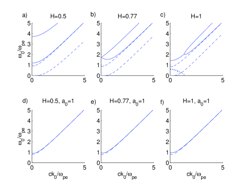
Figure 1: Dispersion curves for the linear and nonlinear propagation of light in Dirac matter for different values of $H=\hbar\omega_{pe}/m_{e}c^{2}$. For the linear cases in a)–c), the solid and dotted curves correspond to solutions using the upper sign in Eq. (37) and dashed curves to solutions with the lower sign in Eq. (37). Panel a) shows a high-frequency branch, the EM branch shifted $\pm H/4$ compared to the plasma frequency at $k_{0}=0$, and a low-frequency branch. For $H>4/3\sqrt{3}\approx 0.77$ the pair branch merge with the upshifted EM branch, and there is an instability for waves with small wavenumbers; the growth rate indicated with the dotted curve for $H=1$. Panels d)–f) shows the dispersion curves for finite amplitude ($a_{0}=1$) EM waves.

In Fig. 1a)–c), we have displayed the solutions of the linear dispersion relation (37), and plotted the dispersion curves for EM waves for different values of $H$. Figure 1a), for $H=0.5$, exhibits a high-frequency pair branch, the two EM branches shifted approximately $\pm H/4$ compared to the plasma frequency at $k_{0}=0$, and a low-frequency branch. For $H=H_{crit}=4/3\sqrt{3}\approx 0.77$, the pair branch merges with the upshifted EM branch for small wavenumbers, as seen in Fig. 1b), and for $H>H_{crit}$ the system exhibits an instability for small wavenumbers. We have plotted the growth rate for the instability for $H=1$ in Fig. 1c. Direct numerical simulations of the Dirac-Maxwell system have confirmed this instability. It leads in the nonlinear stage to an interplay between the $\widetilde{\Psi}_{1}$ and $\widetilde{\Psi}_{4}$ components of the spinor, and the excitation large amplitude ($a_{0}=1$–$2$) oscillatory EM fields. The dispersion relation for a finite amplitude EM wave, shown in Fig. 1d)–f), shows that the frequency is downshifted in the intense EM field, and that the quantum frequency shifts decrease compared to the linear cases. Equation (37) with the lower sign also yields a low-frequency wave, plotted in Figs. 1a)–1c) for $\omega_{0}^{2}\ll c^{2}k_{0}^{2}\ll\omega_{pe}^{2}$, from which we have the low-frequency dispersion relation

$$\omega_{0}=\frac{\hbar c^{2}k_{0}^{4}}{2m_{e}\omega_{pe}^{2}},$$ (38)

which is a low-frequency spin-EM wave. We found that the low-frequency branch exists as a propagating wave only in the weakly relativistic regime, and disappears completely as a propagating wave for $a_{0}\gtrsim 0.24H$. We mention that ion dynamics can become important in the low-frequency range. We mention that ion dynamics can become important in the low-frequency range. For cold fluid ions, Eq. (24) is replaced by $\omega_{0}^{2}-c^{2}k_{0}^{2}=-(\chi_{e}+\chi_{i})\omega_{0}^{2}$ where the ion susceptibility is $\chi_{i}=-\omega_{pi}^{2}/\omega_{0}^{2}$ and $\omega_{pi}$ is the ion plasma frequency, and $\omega_{pi}^{2}$ is added to the right-hand side of Eq. (36). For this case, we retain (38) for $\omega_{pi}^{2}$, $\omega_{0}^{2}\ll c^{2}k_{0}^{2}\ll\omega_{pe}^{2}$, while for $\omega_{0}^{2}\ll c^{2}k_{0}^{2}\ll\omega_{pi}^{2}\ll\omega_{pe}^{2}$, we instead have the low-frequency ion mode $\omega_{0}={\hbar k_{0}^{2}}/{2m_{i}}$ where $m_{i}$ is the ion mass.

III.4.2 The dipole field

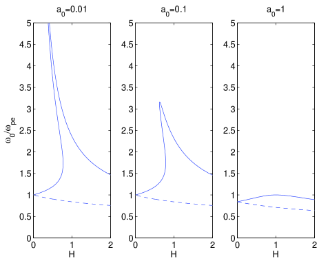
Figure 2: The cutoff frequency $\omega_{0}$ at $K=k_{0}=0$ as a function of $H$ for different values of $a_{0}=eA_{0}/m_{e}c$. The cutoff frequency is upshifted for the spin ’up’ state (solid lines) and downshifted for spin ’down’ (dashed lines). In the classical limit $H\rightarrow 0$, we have $\omega_{0}\rightarrow\omega_{pe}/\sqrt{\gamma_{0}}$ for both spin states, where $\gamma_{0}=\sqrt{1+a_{0}^{2}}$.

It is also possible to find simple expressions for the plasma susceptibility for the dipole case $k_{0}=K=0$ with arbitrary amplitude $A_{0}$, which yields the nonlinear cutoff frequency of the EM wave. Here, inserting $\Psi_{2}=\Psi_{3}=0$ into (14)–(17) yields nontrivial solutions for $\Omega=({1}/{\hbar})\sqrt{(m_{e}c^{2}-{\hbar\omega_{0}}/{2})^{2}+c^{2}e^{2}A_{0}^{2}}$. Equations (14) or (17) then yield the relation between $\Psi_{1}$ and $\Psi_{4}$, which are normalized such that $\Psi_{1}^{2}+\Psi_{4}^{2}=n_{0}$. On the other hand, inserting $\Psi_{1}=\Psi_{4}=0$ into (14)–(17) yields nontrivial solutions for $\Omega=({1}/{\hbar})\sqrt{(m_{e}c^{2}+{\hbar\omega_{0}}/{2})^{2}+c^{2}e^{2}A_{0}^{2}}$. Equations (15) or (16) then yield the relation between $\Psi_{2}$ and $\Psi_{3}$, which are normalized such that $\Psi_{2}^{2}+\Psi_{3}^{2}=n_{0}$. The resulting susceptibility is $\chi_{e}=\chi_{e\pm}$, where

$$\chi_{e\pm}=-\frac{\omega_{pe}^{2}}{\omega_{0}^{2}\gamma_{\pm}},$$ (39)

and we have denoted

$$\gamma_{\pm}=\sqrt{(1\mp\frac{\hbar\omega_{0}}{2m_{e}c^{2}})^{2}+\frac{e^{2}A_{0}^{2}}{m_{e}^{2}c^{2}}},$$ (40)

which, inserted into (24) with $k_{0}=0$, yields

$$\omega_{0}^{2}=\frac{\omega_{pe}^{2}}{\gamma_{\pm}}.$$ (41)

Here $\omega_{0}$ can be seen as the effective plasma frequency in the presence of quantum spin effects and the EM field. We note that the spin effect contributes to a relative frequency shift of the order $\pm\hbar\omega_{pe}/4m_{e}c^{2}$ compared to the classical plasma frequency, while a large amplitude radiation field $A_{0}$ leads to a frequency downshift, which resembles the effect of the relativistic electron mass increase in the classical plasma.

The dependence of $\omega_{0}$ on $H$ has been plotted in Fig. 2 for different values of $a_{0}=eA_{0}/m_{e}c$. We see that the frequency shifts increase linearly with $H$ for $H\ll 1$, while the upshifted branch experiences a sharp rise at $H\approx 0.77$, which is the critical value of $H$ where the upper branch looses its stability according to Fig. 1. We note that the relative quantum shift disappears both in the classical limit $\hbar\rightarrow 0$ and in the non-relativistic limit $c\rightarrow\infty$, hence the relative shift $\hbar\omega_{pe}/4m_{e}c^{2}$ is a combined quantum and relativistic collective effect.

III.4.3 Vacuum case

It is also interesting to consider the vacuum case $\omega_{0}=ck_{0}$, originally considered by Volkov Volkov35 , where we have either $D_{+}=0$ or $D_{-}=0$ in Eq. (18). We consider here ${\bf A}$ as an external field, not influenced by the plasma, and calculate the plasma response. For $D_{+}=0$, the quasi-neutrality and current-neutrality conditions (20) and (22) give $K=-{k_{0}}/{2}=-{\omega_{0}}/{2c}$ and $\Omega=-{\omega_{0}}/{2}+{\gamma_{0}m_{e}c^{2}}/{\hbar}$, and the solutions $\widetilde{\Psi}_{1}=[{(1+\gamma_{0})}/{2\gamma_{0}}]\widetilde{\Psi}_{0}$, $\widetilde{\Psi}_{2}=-({eA_{0}}/{m_{e}c}){\widetilde{\Psi}_{0}}/{2\gamma_{0}}$, $\widetilde{\Psi}_{3}=-({e^{2}A_{0}^{2}}/{m_{e}^{2}c^{2}}){\widetilde{\Psi}_{0}}/{2\gamma_{0}(1+\gamma_{0})}$, and $\widetilde{\Psi}_{4}=({eA_{0}}/{m_{e}c}){\widetilde{\Psi}_{0}}/{2\gamma_{0}}$. If we instead use $D_{-}=0$, then we obtain $K={k_{0}}/{2}={\omega_{0}}/{2c}$, and $\Omega={\omega_{0}}/{2}+{\gamma_{0}m_{e}c^{2}}/{\hbar}$, and the solutions $\widetilde{\Psi}_{1}=({eA_{0}}/{m_{e}c}){\widetilde{\Psi}_{0}}/{2\gamma_{0}}$, $\widetilde{\Psi}_{2}=[{(1+\gamma_{0})}/{2\gamma_{0}}]\widetilde{\Psi}_{0}$, $\widetilde{\Psi}_{3}=({eA_{0}}/{m_{e}c}){\widetilde{\Psi}_{0}}/{2\gamma_{0}}$, and $\widetilde{\Psi}_{4}=({e^{2}A_{0}^{2}}/{m_{e}^{2}c^{2}}){\widetilde{\Psi}_{0}}/{2\gamma_{0}(1+\gamma_{0})}$.

The resulting susceptibility for both cases is

$${\chi}_{e}=-\frac{\omega_{pe}^{2}}{\omega_{0}^{2}\gamma_{0}},$$ (42)

which is identical to the case of the classical plasma where the relativistic gamma factor gives rise to nonlinear effects, such as the self-induced transparency of the EM waves Akhiezer56 . The above result was also obtained in a simplified model Eliasson11 by using the Klein-Gordon equation for spinless particles. Hence, for the vacuum case, there is no difference in plasma response between the two spin states.

IV Extensions to mixed states and kinetic models

In the above investigation, we have considered the idealized case where all electrons have a well-defined spin state. Therefore, these results can be seen as limiting cases of more complicated cases with an admixture of electrons with different spin. The simplest mixed state solution could be achieved by assuming that we have an admixture of the electrons with spin-up and spin-down states. If the electrons are distributed equally among the two spin states (but not among negative energy states), we would instead of (24) have the dispersion relation

$$\omega_{0}^{2}-c^{2}k_{0}^{2}=-\frac{(\chi_{e+}+\chi_{e-})}{2}\omega_{0}^{2},$$ (43)

where $\chi_{e+}$ and $\chi_{e-}$ are the electric susceptibilities obtained by solving the two separate Dirac equations for the two spin states, each normalized according to (20) and fulfilling (22). For example, for the linear case we would use the susceptibilities $\chi_{e\pm}$ in (35) in (43) to construct the dispersion relation

$$\omega_{0}^{2}-c^{2}k_{0}^{2}=-\frac{4\omega_{0}^{2}\omega_{pe}^{2}m_{e}^{2}c^{4}}{\hbar^{2}(\omega_{0}^{2}-c^{2}k_{0}^{2})^{2}-4\omega_{0}^{2}m_{e}^{2}c^{4}},$$ (44)

which can be rewritten as

$$\omega_{0}^{2}-c^{2}k_{0}^{2}-\omega_{pe}^{2}=\frac{\hbar^{2}(\omega_{0}^{2}-c^{2}k_{0}^{2})^{3}}{4\omega_{0}^{2}m_{e}^{2}c^{4}}.$$ (45)

For $\omega_{0}\approx\omega_{pe}$ and $ck_{0}\ll\omega_{pe}$, there is a relative quantum upshift of the frequency of the order $H^{2}/8$, which is extremely small for normal laboratory conditions where $H\ll 1$. On the other hand, for $\omega_{0}^{2}\ll c^{2}k_{0}^{2}\ll\omega_{pe}^{2}$, we have a low-frequency branch $\omega_{0}=\hbar c^{3}k_{0}^{3}/2\omega_{pe}m_{e}c^{2}$. Using a similar procedure for the nonlinear cutoff frequency, the dispersion relation (41) would then be replaced by

$$\omega_{0}^{2}-\frac{\omega_{pe}^{2}}{2}\bigg{(}\frac{1}{\gamma_{+}}+\frac{1}{\gamma_{-}}\bigg{)}=0,$$ (46)

where $\gamma_{\pm}$ are given by (40). More complex, kinetic models can be constructed by extending the dispersion relation (43) to include not only the sum over the two spin states, but also sums (or integrals) over the excited states having different wavenumbers $K$. We like to mention that a kinetic model recently has been derived Mendonca11 to describe wave propagation in a relativistic quantum plasma based on the Klein-Gordon equation and using a Wigner transform technique.

V Summary and conclusions

In this paper, we have studied the nonlinear propagation of light in dense matter by using a collective Dirac model coupled with the Maxwell equations, which includes the nonlinear effects of the finite amplitude EM waves and the electron spin-1/2 effects. As an example, we have considered the nonlinear propagation of circularly polarized EM waves in a quantum plasma, and have studied the effects of different spin polarization, which introduces an up- or down shift of the EM waves, depending on whether the plasma electron is in a spin ’up’ or spin ’down’ state. This relative frequency shift is of the order $10^{-5}$–$10^{-4}$ for typical solid density or compressed density plasmas in the laboratory, but could be much larger in astrophysical settings (e.g. in the core of white dwarf stars), where the plasmonic energy density $\hbar\omega_{pe}$ is comparable to the electron rest energy. The spin related frequency shift could potentially be observed experimentally if a high-density plasma slab Holmlid09 with a definite spin state is irradiated with a laser beam with different polarization. In such a plasma it is also expected that linearly polarized laser light would perform Faraday rotation due to the different dispersive properties of the right-hand and left-hand polarized wave. For laser waves with frequencies between the cutoff frequencies for the right-hand and left-hand polarized wave, the plasma slab would work as a filter and only allow one of the polarizations to propagate through the slab. Above a critical plasma number density, there is a density driven instability, in which the pure spin up or spin down state is unstable under the generation of circularly polarized EM waves. Instabilities of this type could be important in the core of white dwarf stars, if the plasma has been spin polarized by a strong magnetic field.

Appendix A The Dirac equation for circularly polarized EM waves

For the case of circularly polarized EM waves of the form ${\bf A}=A_{0}(\widehat{\bf x}\cos\theta-\widehat{\bf y}\sin\theta)$ where $\theta=k_{0}z-\omega_{0}t$, we seek solutions of the Dirac equation (1) of the form $\psi=\Psi(\theta)\exp(iKz-i\Omega t)$, where we introduced the wavenumber $K$ and frequency $\Omega$ that are related to the momentum and energy of the electrons. This yields the relations

$$\frac{\partial\psi}{\partial t}=-\bigg{(}\omega_{0}\frac{d\Psi}{d\theta}+i\Omega\Psi\bigg{)}\exp(iKz-i\Omega t),$$ (47)

and

$$\nabla\psi=\widehat{\bf z}\bigg{(}k_{0}\frac{d\Psi}{d\theta}+iK\Psi\bigg{)}\exp(iKz-i\Omega t).$$ (48)

The Dirac equation (1) takes the form

$$-i\hbar(\omega_{0}\frac{d\Psi}{d\theta}+i\Omega\Psi)-c\boldsymbol{\alpha}\cdot\bigg{[}-i\hbar\widehat{\bf z}\bigg{(}k_{0}\frac{d\Psi}{d\theta}+iK\Psi\bigg{)}+eA_{0}(\widehat{\bf x}\cos\theta-\widehat{\bf y}\sin\theta)\Psi\bigg{]}-m_{e}c^{2}\beta\Psi=0,$$ (49)

which is a coupled system of 4 ordinary differential equations for $\Psi_{1}$–$\Psi_{4}$. To put it in an explicit form, we evaluate

$$\beta\Psi=\left(\begin{matrix}1&0&0&0\\ 0&1&0&0\\ 0&0&-1&0\\ 0&0&0&-1\end{matrix}\right)\left(\begin{matrix}\Psi_{1}\\ \Psi_{2}\\ \Psi_{3}\\ \Psi_{4}\end{matrix}\right)=\left(\begin{matrix}\Psi_{1}\\ \Psi_{2}\\ -\Psi_{3}\\ -\Psi_{4}\end{matrix}\right)$$ (50)

$$\boldsymbol{\alpha}\cdot\widehat{\bf z}\Psi=\alpha_{z}\Psi=\left(\begin{matrix}0&0&1&0\\ 0&0&0&-1\\ 1&0&0&0\\ 0&-1&0&0\end{matrix}\right)\left(\begin{matrix}\Psi_{1}\\ \Psi_{2}\\ \Psi_{3}\\ \Psi_{4}\end{matrix}\right)=\left(\begin{matrix}\Psi_{3}\\ -\Psi_{4}\\ \Psi_{1}\\ -\Psi_{2}\end{matrix}\right)$$ (51)

and

$$\begin{split}&\boldsymbol{\alpha}\cdot(\widehat{\bf x}\cos\theta-\widehat{\bf y}\sin\theta)\Psi=(\alpha_{x}\cos\theta-\alpha_{y}\sin\theta)\Psi\\ &=\left[\left(\begin{matrix}0&0&0&1\\ 0&0&1&0\\ 0&1&0&0\\ 1&0&0&0\end{matrix}\right)\cos\theta-\left(\begin{matrix}0&0&0&-i\\ 0&0&i&0\\ 0&-i&0&0\\ i&0&0&0\end{matrix}\right)\sin\theta\right]\left(\begin{matrix}\Psi_{1}\\ \Psi_{2}\\ \Psi_{3}\\ \Psi_{4}\end{matrix}\right)=\left(\begin{matrix}e^{i\theta}\Psi_{4}\\ e^{-i\theta}\Psi_{3}\\ e^{i\theta}\Psi_{2}\\ e^{-i\theta}\Psi_{1}\end{matrix}\right).\end{split}$$ (52)

The Dirac equation thus takes the form

$$\big{[}-i\hbar(\omega_{0}\frac{d}{d\theta}+i\Omega)-m_{e}c^{2}\big{]}\Psi_{1}+ic\hbar(k_{0}\frac{d}{d\theta}+iK)\Psi_{3}-ceA_{0}e^{i\theta}\Psi_{4}=0$$ (53)

$$\big{[}-i\hbar(\omega_{0}\frac{d}{d\theta}+i\Omega)-m_{e}c^{2}\big{]}\Psi_{2}-ic\hbar(k_{0}\frac{d}{d\theta}+iK)\Psi_{4}-ceA_{0}e^{-i\theta}\Psi_{3}=0$$ (54)

$$\big{[}-i\hbar(\omega_{0}\frac{d}{d\theta}+i\Omega)+m_{e}c^{2}\big{]}\Psi_{3}+ic\hbar(k_{0}\frac{d}{d\theta}+iK)\Psi_{1}-ceA_{0}e^{i\theta}\Psi_{2}=0$$ (55)

$$\big{[}-i\hbar(\omega_{0}\frac{d}{d\theta}+i\Omega)+m_{e}c^{2}\big{]}\Psi_{4}-ic\hbar(k_{0}\frac{d}{d\theta}+iK)\Psi_{2}-ceA_{0}e^{-i\theta}\Psi_{1}=0$$ (56)

To eliminate the $e^{i\theta}$ and $e^{-i\theta}$ phase factors, we assume $\Psi_{1}=\widetilde{\Psi}_{1}e^{i\theta/2}$, $\Psi_{2}=\widetilde{\Psi}_{2}e^{-i\theta/2}$, $\Psi_{3}=\widetilde{\Psi}_{3}e^{i\theta/2}$, and $\Psi_{4}=\widetilde{\Psi}_{4}e^{-i\theta/2}$, where $\widetilde{\Psi}_{1}$–$\widetilde{\Psi}_{4}$ are constants, to obtain

$$\big{[}\hbar(\Omega+\frac{\omega_{0}}{2})-m_{e}c^{2}\big{]}\widetilde{\Psi}_{1}-c\hbar(K+\frac{k_{0}}{2})\widetilde{\Psi}_{3}-ceA_{0}\widetilde{\Psi}_{4}=0$$ (57)

$$\big{[}\hbar(\Omega-\frac{\omega_{0}}{2})-m_{e}c^{2}\big{]}\widetilde{\Psi}_{2}+c\hbar(K-\frac{k_{0}}{2})\widetilde{\Psi}_{4}-ceA_{0}\widetilde{\Psi}_{3}=0$$ (58)

$$\big{[}\hbar(\Omega+\frac{\omega_{0}}{2})+m_{e}c^{2}\big{]}\widetilde{\Psi}_{3}-c\hbar(K+\frac{k_{0}}{2})\widetilde{\Psi}_{1}-ceA_{0}\widetilde{\Psi}_{2}=0$$ (59)

$$\big{[}\hbar(\Omega-\frac{\omega_{0}}{2})+m_{e}c^{2}\big{]}\widetilde{\Psi}_{4}+c\hbar(K-\frac{k_{0}}{2})\widetilde{\Psi}_{2}-ceA_{0}\widetilde{\Psi}_{1}=0,$$ (60)

where $\Omega$ takes the role of an eigenvalue. The coefficient matrix is real and symmetric, hence $\Omega$ is real and $\widetilde{\Psi}_{j}$ can also be assumed real.

Appendix B Derivation of the electron current

The $x$, $y$ and $z$ components of the current density

$${\bf j}_{e}=-ec\psi^{\dagger}\boldsymbol{\alpha}\psi=-ec(\psi^{\dagger}\alpha_{x}\psi\widehat{\bf x}+\psi^{\dagger}\alpha_{y}\psi\widehat{\bf y}+\psi^{\dagger}\alpha_{z}\psi\widehat{\bf z}),$$ (61)

are obtained with the help of the expressions (See Appendix A for the relation between $\psi_{j}$ and $\widetilde{\Psi}_{j}$)

$$\begin{split}\psi^{\dagger}\alpha_{x}\psi&=\left(\begin{matrix}\psi_{1}^{\ast}&\psi_{2}^{\ast}&\psi_{3}^{\ast}&\psi_{4}^{\ast}\end{matrix}\right)\left(\begin{matrix}0&0&0&1\\ 0&0&1&0\\ 0&1&0&0\\ 1&0&0&0\end{matrix}\right)\left(\begin{matrix}\psi_{1}\\ \psi_{2}\\ \psi_{3}\\ \psi_{4}\end{matrix}\right)=\psi_{1}^{\ast}\psi_{4}+\psi_{2}^{\ast}\psi_{3}+\psi_{3}^{\ast}\psi_{2}+\psi_{4}^{\ast}\psi_{1}\\ &=(\widetilde{\Psi}_{1}\widetilde{\Psi}_{4}+\widetilde{\Psi}_{3}\widetilde{\Psi}_{2})(e^{i\theta}+e^{-i\theta})=2(\widetilde{\Psi}_{1}\widetilde{\Psi}_{4}+\widetilde{\Psi}_{3}\widetilde{\Psi}_{2})\cos(\theta),\end{split}$$ (62)

$$\begin{split}\psi^{\dagger}\alpha_{y}\psi&=\left(\begin{matrix}\psi_{1}^{\ast}&\psi_{2}^{\ast}&\psi_{3}^{\ast}&\psi_{4}^{\ast}\end{matrix}\right)\left(\begin{matrix}0&0&0&-i\\ 0&0&i&0\\ 0&-i&0&0\\ i&0&0&0\end{matrix}\right)\left(\begin{matrix}\psi_{1}\\ \psi_{2}\\ \psi_{3}\\ \psi_{4}\end{matrix}\right)=-i\psi_{1}^{\ast}\psi_{4}+i\psi_{2}^{\ast}\psi_{3}-i\psi_{3}^{\ast}\psi_{2}+i\psi_{4}^{\ast}\psi_{1}\\ &=i(\widetilde{\Psi}_{1}\widetilde{\Psi}_{4}+\widetilde{\Psi}_{3}\widetilde{\Psi}_{2})(e^{i\theta}-e^{-i\theta})=-2(\widetilde{\Psi}_{1}\widetilde{\Psi}_{4}+\widetilde{\Psi}_{3}\widetilde{\Psi}_{2})\sin(\theta),\end{split}$$ (63)

and

$$\begin{split}\psi^{\dagger}\alpha_{z}\psi&=\left(\begin{matrix}\psi_{1}^{\ast}&\psi_{2}^{\ast}&\psi_{3}^{\ast}&\psi_{4}^{\ast}\end{matrix}\right)\left(\begin{matrix}0&0&1&0\\ 0&0&0&-1\\ 1&0&0&0\\ 0&-1&0&0\end{matrix}\right)\left(\begin{matrix}\psi_{1}\\ \psi_{2}\\ \psi_{3}\\ \psi_{4}\end{matrix}\right)=\psi_{1}^{\ast}\psi_{3}-\psi_{2}^{\ast}\psi_{4}+\psi_{3}^{\ast}\psi_{1}-\psi_{4}^{\ast}\psi_{2}\\ &=2(\widetilde{\Psi}_{1}\widetilde{\Psi}_{3}-\widetilde{\Psi}_{2}\widetilde{\Psi}_{4}),\end{split}$$ (64)

respectively, giving

$${\bf j}_{e}=-2ec[(\widetilde{\Psi}_{1}\widetilde{\Psi}_{4}+\widetilde{\Psi}_{3}\widetilde{\Psi}_{2})(\widehat{\bf x}\cos\theta-\widehat{\bf y}\sin\theta)+(\widetilde{\Psi}_{1}\widetilde{\Psi}_{3}-\widetilde{\Psi}_{2}\widetilde{\Psi}_{4})\widehat{\bf z}].$$ (65)

References

• (1) R. Bingham, Nature (London) 424, 258 (2003).
• (2) S. P. D. Mangles et al., Nature (London) 431, 535 (2004); C. G. R. Geddes et al., Nature (London) 431, 538 (2004); J. Faure et al., Nature (London) 431, 541 (20043).
• (3) E. Hand, Nature (London) 461, 708 (2009).
• (4) S. H. Glenzer et al., Phys. Rev. Lett. 98, 065002 (2007); P. Neumayer et al., ibid. 105, 075003 (2010); S. H. Glenzer and R. Redmer, Rev. Mod. Phys. 81, 1625 (2009).
• (5) A. V. Andreev, JETP Lett. 72, 238 (2000).
• (6) G. Mourou et al., Rev. Mod. Phys. 78, 309 (2006).
• (7) M. Marklund and P. K. Shukla, Rev. Mod. Phys. 78, 591 (2006).
• (8) A. Serbeto, J. T. Mendonça, K. H. Tui et al., Phys. Plasmas 15, 013110 (2008).
• (9) A. Serbeto, L. F. Monteiro, K. H. Tsui, and J. T. Mendonça, Plasma Phys. Control. Fusion 51 124024 (2009).
• (10) N. Piovella, M. M. Cola, L. Volpe, A. Schiavi, R. Bonifacio, Phys. Rev. Lett. 100, 044801 (2008).
• (11) A. P. Mills, Jr., D. B. Cassidy, and R. G. Greaves, Mater. Sci. Forum 445, 424 (2004).
• (12) D. B. Cassidy and A. P. Mills, Jr., Nature 449, 195 (2007); D. B. Cassidy, V. E. Meligne, and A. P. Mills, Jr., Phys. Rev. Lett. 104, 173401 (2010).
• (13) E. V. Tkalya, Phys. Rev. Lett. 106, 162501 (2011).
• (14) G. Chabrier et al., J. Phys.: Condens. Matter 14, 9133 (2002); J. Phys. A: Math. Gen. 39, 4411 (2006).
• (15) M. J. Coe et al., Nature (London) 272, 37 (1978); D. K. Galloway and J. L. Sokoloski, Astrophys. J. 613, L61 (2004).
• (16) K. Hurley et al., Nature (London) 434, 1098 (2005); A. K. Harding and D. Lai, Rep. Prog. Phys. 69 2631 (2006).
• (17) V. N. Tsytovich, Sov. Phys. JETP 13, 1249 (1961).
• (18) B. Jancovici, Nuovo Cimento 25, 428 (1962).
• (19) R. Hakim and J. Heyvaerts, Phys. Rev. A 18, 1250 (1978).
• (20) R. Hakim, Riv. Nuovo Cimento 1, 1 (1978).
• (21) R. Hakim and J. Heyvaerts, J. Phys. A: Math. Gen. 13, 2001 (1980).
• (22) H. D. Sivak, Ann. Phys. 159, 351 (1985).
• (23) A. E. Delsante and N. E. Frankel, Ann. Phys. (NY) 125, 135 (1980).
• (24) V. Kowalenko, N. E. Frankel, and K. C. Hines, Phys. Rep. 126, 109 (1985).
• (25) L. M. Hayes and D. B., Melrose, Aust. J. Phys. 37, 615 (1984).
• (26) D. B. Melrose and L. M. Hayes, Aust. J. Phys. 37, 639 (1984).
• (27) D. B. Melrose, J. I. Weise, and McOrist, J. Phys. A: Math. Gen. 39, 8727 (2006).
• (28) F. A. Asenjo, V. Muñoz, J. A. Valdivia, and S. M. Mahajan, Phys. Plasmas 18, 012107 (2011).
• (29) T. Takabayasi, Prog. Theor. Phys. 13, 222 (1955); Phys. Rev. 102, 297 (1956); Nuovo Ciemento 3, 233 (1956); Prog. Theor. Phys. Suppl. 4, 2 (1957).
• (30) A. I. Akhiezer and R. V. Polovin, Sov. Phys. JETP 3, 696 (1956) [Zh. Eksp. Teor. Fiz. 30, 915 (1956)]; P. Kaw and J. Dawson, Phys. Fluids 13, 472 (1970); C. Max and F. Perkins, Phys. Rev. Lett. 27, 1342 (1971).
• (31) P.K. Shukla et al., Phys. Rep. 138, 1 (1986).
• (32) C. J. McKinstrie and R. Bingham, Phys. Fluids B 1, 230 (1989).
• (33) L. N. Tsintsadze, Sov. J. Plasma Phys. 17, 872 (1991).
• (34) L. Gross, Commun. Pure Appl. Math. 19, 1 (1996); J. M. Chadam, J. Math. Phys. 13, 597 (1972); J. C. H. Simon, Lett. Math. Phys. 6, 487 (1982); A. Das, J. Math. Phys. 34, 3986 (1993).
• (35) V. M. Malkin, N. J. Fisch, and J. S. Wurtele, Phys. Rev. E 75, 026404 (2007).
• (36) D. M. Volkov, Z. Phys. 94, 250 (1935); J. T. Mendonça and A. Serbeto, Phys. Rev. E 83, 026406 (2011).
• (37) F. S. Felber and J. H. Marburger, J. Math. Phys. 16, 2089 (1975).
• (38) R. Kodama et al., Nature 412, 798 (2001).
• (39) H. Azechi et al., Laser Part. Beams 9, 193 (1991).
• (40) L. Holmlid, H. Hora, G. Miley and X. Yang, Laser Part. Beams 27, 529 (2009).
• (41) B. Eliasson and P. K. Shukla, Phys. Rev. E 83, 046407 (2011).
• (42) J. T. Mendonça, Phys. Plasmas 18, 062101 (2011).