Accretion in the detached post-common-envelope binary LTT 560

In a previous study, we found that the detached post-common-envelope binary LTT 560 displays an H$\alpha$ emission line consisting of two anti-phased components. While one of them was clearly caused by stellar activity from the secondary late-type main-sequence star, our analysis indicated that the white dwarf primary star is potentially the origin of the second component. However, the low resolution of the data means that our interpretation remains ambiguous. We here use time-series UVES data to compare the radial velocities of the H$\alpha$ emission components to those of metal absorption lines from the primary and secondary stars. We find that the weaker component most certainly originates in the white dwarf and is probably caused by accretion. An abundance analysis of the white dwarf spectrum yields accretion rates that are consistent with mass loss from the secondary due to a stellar wind. The second and stronger H$\alpha$ component is attributed to stellar activity on the secondary star. An active secondary is likely to be present because of the occurrence of a flare in our time-resolved spectroscopy. Furthermore, Roche tomography indicates that a significant area of the secondary star on its leading side and close to the first Lagrange point is covered by star spots. Finally, we derive the parameters for the system and place it in an evolutionary context. We find that the white dwarf is a very slow rotator, suggesting that it has had an angular-momentum evolution similar to that of field white dwarfs. We predict that LTT 560 will begin mass transfer via Roche-lobe overflow in $\sim$3.5 Gyrs, and conclude that the system is representative of the progenitors of the current population of cataclysmic variables. It will most likely evolve to become an SU UMa type dwarf nova.

1 Introduction

Cataclysmic variables (CVs) are thought to form from detached white dwarf (WD) / main-sequence star (MS) binaries that have experienced a common-envelope (CE) phase (e.g., Taam & Ricker, 2010; Webbink, 2008). In these “post-common-envelope binaries” (PCEBs), the white dwarf represents the more massive component in the system and is therefore called the primary, while the usually late-type (K–M) main-sequence star is known as the secondary. After the end of the CE phase, angular-momentum loss due to magnetic braking and/or gravitational radiation continues to decrease the separation between the two stars. This eventually brings the secondary’s Roche lobe into contact with the stellar surface, thus initiating stable mass-transfer via Roche-lobe overflow and the semi-detached CV phase (Ritter, 2008, and references therein).

There is growing evidence that the accretion of material from the secondary star does not start with Roche-lobe overflow. The discovery of so-called “low accretion rate polars” (Schwope et al., 2002), which are likely progenitors of magnetic CVs (Schmidt et al., 2005, 2007), and the detection of metal absorption lines in the UV spectra of non-magnetic PCEBs (e.g., Kawka et al., 2008), indicate that wind accretion from the active chromosphere of the secondary star is a common phenomenon in detached, short-period, WD/MS binaries.

Tappert et al. (2007, hereafter Paper I) found the H$\alpha$ emission line in the detached PCEB LTT 560 to be a combination of two components. The radial velocity variations in the stronger H$\alpha$ component agree well with those shown by the TiO absorption, and was thus identified as originating in the secondary star. The radial velocities of the weaker component showed an – within the errors – anti-phased behaviour with respect to the secondary star exhibiting a lower amplitude, and therefore had to be produced on the side of the centre-of-mass opposite to the secondary. However, the low spectral resolution of the data, and the contamination of the white-dwarf Balmer absorption lines with emission cores from the secondary, impeded velocity measurements of other, unambiguously intrinsic, spectral features from the white dwarf. Thus, the true origin of the weak emission component remained unresolved. The low temperature of the white dwarf in LTT 560 ($T\sim 7500\leavevmode\nobreak\ \mathrm{K}$, Paper I) and the evidence of ongoing accretion imply that there is a high probability that there are narrow metal absorption lines in the white-dwarf spectrum (Zuckerman et al., 2003). The radial velocity curve of such lines should be undisturbed and thus faithfully track the motion of the white dwarf, motivating the high-resolution study presented in this paper.

2 Observations and data reduction

LTT 560 was observed on August 16, 2007 using UVES on UT1 (ANTU) at ESO Paranal. A total of 38 Echelle spectra was taken over 7.3 h in one blue (3260–4528 Å) and two red (5681-7519 Å, 7661-9439 Å, hereafter ”lower” and ”upper” red spectrum, respectively) spectral ranges, with resolving power $\sim$70 000. The exposure time per spectrum was 600 s, which corresponds to roughly 0.05 orbital cycles. The sequence of time-resolved spectra had to be interrupted for about 45 min when the object was close to the zenith, where the VLT cannot observe.

The data reduction was performed using Gasgano and the UVES pipeline (version 3.9.0) in a step-by-step mode. This included bias and flat correction, wavelength calibration with a ThAr lamp, and flux calibration using the standard star LTT 7987. The response function proved rather unsatisfactory, with the flux-calibrated spectra still containing several ”order wriggles”. However, since this bears no relevance to the work described in this paper, we did not attempt to resolve this issue.

3 Results

Figure 1: Selected ranges of the blue spectrum with line identifications. This average spectrum has been produced by combining 38 individual spectra that had each been corrected for the radial velocity variations of the white dwarf.

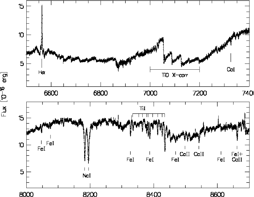
Figure 2: Selected ranges of the average red spectra. The respective individual spectra have been corrected for the radial velocities of the secondary star. The spectra are not corrected for telluric contamination. Indicated are the H$\alpha$ emission line, the spectral range that has been used for the cross-correlation, and the absorption lines that could be unambiguously identified.

In Figs. 1 and 2, we present selected wavelength ranges of the averaged blue and red spectra. For the computation of both spectra, the individual data were corrected for the motion of the respective components based on the radial velocity parameters derived in Section 3.1. Thus, Fig. 1 shows the blue spectrum in the rest frame of the white dwarf, while Fig. 2 gives the red spectra in the rest frame of the late M dwarf. Absorption features of both stellar components were identified using the ILLSS catalogue (Coluzzi, 1999).

The two red spectra are dominated by the features of the secondary star, which are mainly molecular TiO bands, but also several atomic absorption lines such as Ca I $\lambda$7326 (in the ”lower” red spectrum), the Na I $\lambda\lambda$8183/8194 doublet, K I, Fe I, Ti I, and Ca II (in the ”upper” red spectrum). As shown in Paper I, the red spectrum is consistent with an M5–6V secondary star. The blue portion of the spectra presents a plethora of narrow metal absorption lines: these are mostly of Fe I, but also Ni I, Si I, Mg I, Al I, Ca I, and Cr I can be identified. In addition, there are the broader lines of Ca II, and H I. In Section 3.2, we use the absorption lines of the white dwarf to estimate the accretion rate.

3.1 Radial velocities

Table 1: Radial velocity parameters.

Feature	$K$	$\gamma$	$\varphi$
	[km s-1]	[km s-1]	[orbits]
H$\alpha_{\mathrm{MS}}$	231.50$\pm$0.51	35.01$\pm$0.46	$-$0.00271(65)
Na I $\lambda$8183	233.72$\pm$0.33	35.59$\pm$0.24	0.00011(24)
Na I $\lambda$8195	228.92$\pm$0.29	37.96$\pm$0.22	$-$0.00019(22)
TiO cc+$\lambda_{0}$	231.17$\pm$0.19	37.18$\pm$1.28	0.00009(14)
H$\alpha_{\mathrm{WD}}$	72.70$\pm$0.15	55.69$\pm$0.14	0.50198(62)
metalav	72.63$\pm$0.88	54.24$\pm$0.88	0.5009(20)
metal cc+$\lambda_{0}$	72.62$\pm$0.16	55.20$\pm$0.74	0.50018(37)

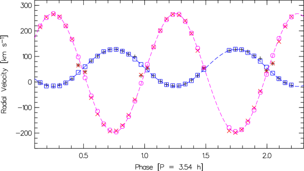
Figure 3: Radial velocities of several spectral features plotted against orbital phase. The latter are presented in sequence, i.e. corresponding to their time of measurement. The plot shows the radial velocities for the broad and narrow H$\alpha$ components (marked by slanted and straight crosses, respectively), and the TiO and metal cross-correlation velocities (circles and squares, resp.). The plot also includes the radial velocity curves calculated from the adapted average radial velocity parameters.

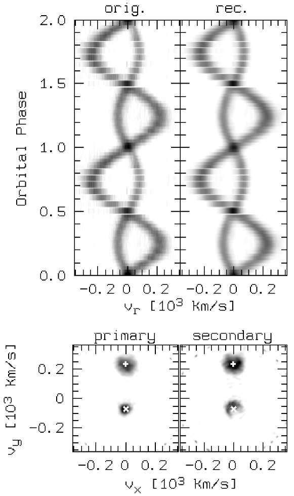
Figure 4: Trailed spectra and Doppler maps. The lower left plot presents the Doppler map corrected for $\gamma_{\mathrm{WD}}$, the lower right plot the corresponding one corrected for $\gamma_{\mathrm{MS}}$. The slanted and the straight cross mark the calculated positions of the stars, i.e.  $K_{\mathrm{WD}}$ and $K_{\mathrm{MS}}$, respectively. The upper plots show the trailed spectra for $\gamma_{\mathrm{WD}}$. The left spectrum represents the original data, the right spectrum is the reconstructed data from the Doppler map. The data are repeated for a second orbital cycle for clarity.

Table 2: System parameters of LTT 560.

WD	$P_{\mathrm{orb}}$	$M_{\mathrm{WD}}$	$M_{\mathrm{MS}}$	$q$	$i$	$a$
	[h]	[$M_{\odot}$]	[$M_{\odot}$]		[∘]	[$R_{\odot}$]
He	3.54(7)	0.46(1)	0.146(4)	0.314(1)	63(2)	1.00(1)
CO	3.54(7)	0.44(1)	0.139(4)	0.314(1)	65(2)	0.98(1)

We recall that the main motivation of the present work was to determine the origin of the two H$\alpha$ emission components. This can be achieved by calculating the parameters of their respective radial velocity variations

$$v_{r}(t)=\gamma+K\sin[2\pi(t-T_{0})/P_{\mathrm{orb}}],$$ (1)

and by comparing them to the corresponding parameters of intrinsic stellar absorption features. We therefore measured the radial velocities of the following lines and spectral regions:
(1)  The two H$\alpha$ emission components were fitted individually with a single Gaussian. For the calculation of the parameters, we excluded the data close to superior and inferior conjunction, when both components merge.
(2)  By fitting single Gaussians again, the velocities for 29 metal absorption lines in the blue spectral range (in the majority Fe I) were measured, and the fitting of sine functions according to Eq. 1 yielded the corresponding parameters. The sample was subsequently restricted to 16 curves with a standard deviation $<0.5\leavevmode\nobreak\ \mathrm{km/s}$ in $\gamma$ to provide average parameters.
(3)  The Na I lines were also measured with single Gaussian functions. An attempt to fit both lines simultaneously with two Gaussians at a fixed separation was unsuccessful because of the irregular and variable continuum.
(4)  Cross-correlation was performed for the spectral ranges 3810–3870 Å (containing several narrow absorption lines) and 7000–7200 Å (including three strong TiO absorption bands). Lacking a proper radial velocity standard, the spectra were correlated to one spectrum of the data set of high signal-to-noise ratio (S/N). The resulting velocities were then fitted according to Eq. 1 with $\gamma$ set to 0. Subsequently, the individual spectra were corrected for the corresponding variation and averaged to yield high S/N spectra. Finally, $\gamma$ was determined by calculating the shift of spectral features with respect to their rest-frame wavelength in these average spectra. For the blue range, this shift was calculated as the average of the positions of 31 lines. For the red range, the Ca I $\lambda$7326 line was used from the lower red spectrum and 12 lines from the upper red range.

Table 1 summarises the resulting parameters. The zero point of the orbital variation $T_{0}$ was set to the inferior conjunction of the TiO cross-correlation velocities, yielding an ephemeris

$$T_{0}({\rm HJD})=2\,454\,329.6840(29)+0.1475(29)\leavevmode\nobreak\ E,$$ (2)

where $E$ is the cycle number. The value for the orbital period was taken from Paper I.

As can be seen in Table 1, and is visualised in Fig. 3, there is a close agreement between all parameters for the respective features of both the white dwarf and the secondary star. We may thus calculate the weighted averages for these parameters:

$$\gamma_{\mathrm{WD}}=55.45(34)\leavevmode\nobreak\ \mathrm{km/s}, K_{\mathrm{WD}}=72.66(11)\leavevmode\nobreak\ \mathrm{km/s},$$

$$\gamma_{\mathrm{MS}}=36.51(72)\leavevmode\nobreak\ \mathrm{km/s}, K_{\mathrm{MS}}=231.22(95)\leavevmode\nobreak\ \mathrm{km/s}.$$

With this, we derive the mass ratio

$$q=K_{\mathrm{WD}}/K_{\mathrm{MS}}=0.3143(13)$$

and the gravitational redshift of the white dwarf

$$v_{\mathrm{gr}}=\gamma_{\mathrm{WD}}-\gamma_{\mathrm{MS}}=18.94(80)\leavevmode\nobreak\ \mathrm{km/s}.$$

These values are consistent with those determined in Paper I ($q=0.36(03)$, $v_{\mathrm{gr}}=25(09)\leavevmode\nobreak\ \mathrm{km/s}$), but represent a vast improvement in accuracy. Assuming a He-core and a CO-core white dwarf, and adopting the mass-radius relations from Panei et al. (2000) for a $10^{-5}\mbox{$M_{\odot}$}$ hydrogen envelope, the gravitational redshift corresponds to $M_{\mathrm{wd}}=0.46\pm 0.12\mbox{$M_{\odot}$}$ and $M_{\mathrm{wd}}=0.44\pm 0.12\mbox{$M_{\odot}$}$, respectively. The resulting updated system parameters (see Paper I for details) are summarised in Table 2.

In Fig. 4, we show the trailed spectrum and the Doppler map that was computed using the fast maximum entropy algorithm of Spruit (1998). The flare data (Section 3.3.1) were excluded, since Doppler tomography does not take into account non-orbital variations. The resulting map represents a two-dimensional visualisation of the emission distribution in velocity space (Marsh & Horne, 1988). We note that the significant difference in the $\gamma$ velocities caused by the gravitational redshift of the white dwarf requires the calculation of two maps with respective corrections. Consequently, the emission from the secondary star appears distorted in the $\gamma_{\mathrm{WD}}$ corrected map, and vice versa. We note that both the emission component from the white dwarf and the one from the secondary star in their respective ”$\gamma$ rest frames” are symmetrically centred on the calculated positions of the stellar components, and that these two are the only H$\alpha$ emitters in the system, i.e. no accretion stream or disc is visible in H$\alpha$.

3.2 The photospheric white dwarf spectrum

Table 3: Photospheric white dwarf abundances.

Element	$\log[\mathrm{X/H}]_{\mathrm{LTT560}}$	$\log[\mathrm{X/H}]_{\odot}$	$\times$solar
Mg	-6.2	-4.4	0.015
Al	-7.6	-5.6	0.010
Si	-6.2	-4.5	0.018
Ca	-7.5	-5.7	0.015
Sc	-10.9	-8.8	0.008
Mn	-8.2	-6.6	0.018
Fe	-6.3	-4.5	0.018
Co	-8.8	-7.0	0.018
Ni	-7.9	-5.8	0.007

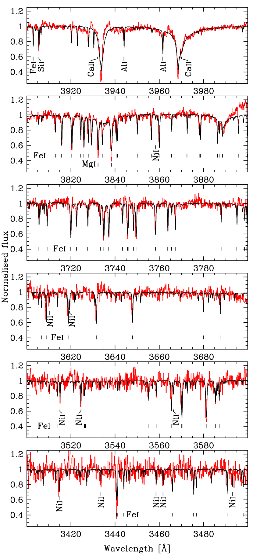
Figure 5: The plethora of metal absorption lines in the average spectrum of the white dwarf in LTT 560 were fitted with TLUSTY/SYNSPEC models to determine the metal abundances in the white dwarf photosphere. The overplotted black line shows a model for $T_{\mathrm{WD}}=7500$ K, $\log g=7.75$, and adopting the abundances listed in Table 3.

We used TLUSTY200 and SYNSPEC48 (Hubeny & Lanz, 1995; Lanz & Hubeny, 1995) along with the Kuruz line list (CD-ROM23) to model the plethora of photospheric metal lines detected in the average UVES spectrum of the white dwarf in LTT 560. The atmospheric models were computed adopting the mixing length version ML2 and a mixing length of 0.6. We fixed the effective temperature to $T_{\mathrm{eff}}=7500$ K, as determined from our analysis of the near-ultraviolet to infrared spectral energy distribution of LTT 560 (Paper I), and $\log g=7.75$, corresponding to the mass determined here. We restrict this analysis to wavelengths below 4000 Å, where the contribution of the companion star is practically zero, hence the photospheric absorption lines from the white dwarf are not contaminated. We identified transitions of Mg, Al, Si, Ca, Sc, Mn, Fe, Co, and Ni, and varied the individual abundances of these elements to achieve the closest fit to the observed line profiles (Fig. 5). The abundances determined from this fit are reported in Table 3, with typical uncertainties of 0.2 dex. Within these uncertainties, the observed abundance pattern is broadly consistent with a solar element mixture at $\simeq 0.015$ times the solar metal abundances (Asplund et al., 2009).

The relatively large abundances of metals in the photosphere of the white dwarf clearly indicate that it is accreting from its companion star. Doppler tomography rules out Roche-lobe overflow, hence the origin of the accreted material is very likely to be the wind of the companion star. Assuming that the white dwarf photosphere is in a steady-state of accretion-diffusion, we can use the determined metal abundances to infer the accretion rate from

$$\dot{M}=\frac{qM_{\mathrm{WD}}X}{\tau_{\mathrm{D}}X_{\mathrm{acc}}},$$ (3)

where $q$ is the mass fraction of the convection zone (in which the accreted material is mixed), $\tau_{\mathrm{D}}$ is the diffusion timescale on which accreted metals drop out of the convection zone, and $[X/H]$ and $[X/H]_{\mathrm{acc}}$ are the abundances observed in the white dwarf atmosphere and in the accreted material, respectively (Dupuis et al., 1993; Koester & Wilken, 2006). We assume that the white dwarf in LTT 560 accretes solar abundance material, and estimate $q=-8.2$ from the plots in Althaus & Benvenuto (1998). Koester & Wilken (2006) list the diffusion timescales for Ca, Mg, and Fe for a wide range of effective temperatures and surface gravities. We interpolate their Table 2 for $T_{\mathrm{WD}}=7500$ K and $\log g=7.75$ to find $\tau_{\mathrm{D}}(\mathrm{Ca})=9400$ yr, $\tau_{\mathrm{D}}(\mathrm{Mg})=9950$ yr, and $\tau_{\mathrm{D}}(\mathrm{Fe})=7460$ yr. Using the abundances of Ca, Mg, and Fe determined from our fits to the photospheric metal lines (Table 3), we obtain three independent estimates of the accretion rate, $\dot{M}=4.4\times 10^{-15}\mbox{$M_{\odot}$}\mathrm{yr^{-1}}$, $4.5\times 10^{-15}\mbox{$M_{\odot}$}\mathrm{yr^{-1}}$, and $\dot{M}=6.0\times 10^{-15}\mbox{$M_{\odot}$}\mathrm{yr^{-1}}$. Within the uncertainties of our analysis, we conclude that the accretion rate onto the white dwarf is $\sim 5\times 10^{-15}\mbox{$M_{\odot}$}\mathrm{yr^{-1}}$.

3.3 Activity

3.3.1 Flaring

Figure 6: Comparison of the two half orbits corresponding to the phase intervals 0.64–1.0 (left panel) and 1.64–2.0 (right) in Fig. 3. The H$\alpha$ component from the secondary star is clearly stronger at the start of the second panel, while the one from the white dwarf remains unchanged.

Figure 7: Equivalent widths of the H$\alpha$ after the emission component of the white dwarf had been subtracted from the spectrum. Open circles mark spectra where the subtraction left significant negative residuals.

In the second part of the second orbit covered by our data, the H$\alpha$ component from the late-type star is significantly enhanced from phases 1.7–1.9, i.e.  immediately after the ”zenith break” (Fig. 6). In contrast, the white-dwarf H$\alpha$ component remains constant. For a quantitative analysis, we measured the equivalent width of the secondary’s H$\alpha$ component as follows. First, we fitted single Gaussian functions to the line profile of the white-dwarf H$\alpha$ component in all spectra where this component was sufficiently isolated. Subsequently, all fits were subtracted from all spectra, and the quality of the subtraction was evaluated visually. Eight fits were found to leave sufficiently negligible residuals. Finally, the equivalent widths of the secondary’s H$\alpha$ component was measured in all eight sets of subtracted spectra.

For four spectra, none of the subtracted line profiles were of satisfactory quality, containing significant negative residuals. Interestingly, three of those represent all the spectra in the phase interval 0.9–1.0, and one might speculate that at these phases (close to superior conjunction of the primary) the white-dwarf H$\alpha$ component is affected by some sort of obscuration. Nevertheless, our coverage here is insufficient for an in-depth analysis, and more data will be needed to confirm this apparent diminished strength of the white-dwarf H$\alpha$ component.

The average equivalent widths are plotted in Fig. 7. The secondary’s H$\alpha$ component at second quadrature during the second observed orbit is clearly about 1.6 times stronger than during the first orbit. The observed maximum of this flare occurs at phase 1.7, but since the phase interval 1.5–1.7 was not covered because of the zenith break it is possible that the real maximum was reached before we recommenced observations. From phase 1.7 to the end of observations at phase 2.2, the strength of the H$\alpha$ line had declined, but had not yet reached its ”quiescence” value at this point. We furthermore note that during the first observed orbit the equivalent width has a local maximum at second quadrature, where it is about 1.4 times larger than at both observed ”unflared” first quadratures (phases 0.25 and 1.25). This indicates that there is an active region on the leading side of the secondary star.

3.3.2 Roche tomography

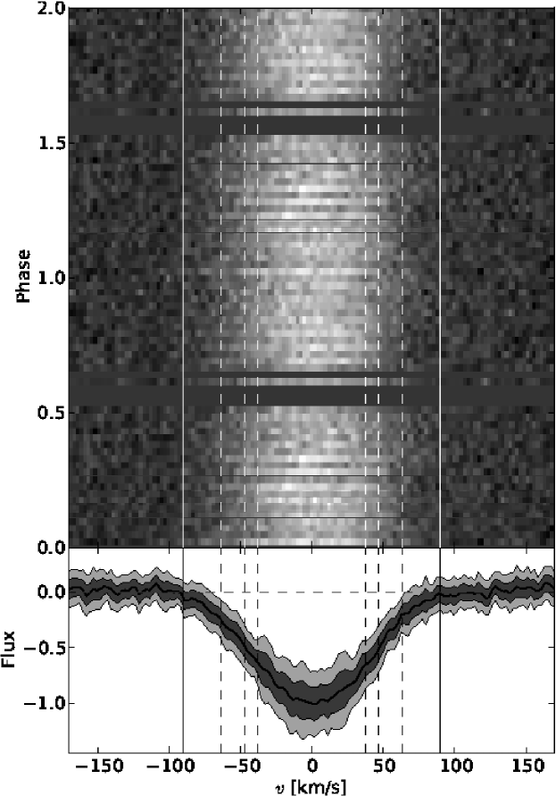
Figure 8: Radial velocity-corrected trailed spectrum (top) and the combined absorption line (bottom) resulting from the least square deconvolution for the data before the zenith break. Dark and light grey regions on the average line profile at the bottom panel show the 1-$\sigma$ and 2-$\sigma$ of the standard deviation throughout the orbit, respectively. Solid vertical lines depict the maximum allowed radius for the secondary star (i.e., its Roche-lobe radius $R_{\rm L1}$). The vertical dashed lines mark the estimated radius $R_{\mathrm{MS}}$ (central lines) and the corresponding 1-$\sigma$ confidence levels obtained from the RT by the $\chi^{2}$ landscape technique.

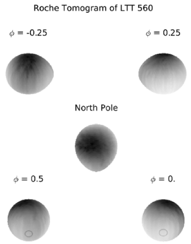
Figure 9: The surface brightness distribution of the secondary star of LTT 560 as derived from the Roche tomography. The L1 face of the star is seen at phase 0.5. The circles mark a region around L1 (lower left plot: seen from the front side; lower right plot: seen through the star). Dark regions represent diminished absorption features of the line profiles, interpreted as spotted regions.

To explore the secondary’s signatures of stellar activity, we used the method of Roche tomography (RT; Rutten & Dhillon, 1994; Watson & Dhillon, 2001), applying an image reconstruction technique to obtain a brightness distribution of the secondary star. This method is based on the maximum entropy regularisation technique (Skilling & Bryan, 1984), which searches for the most featureless brightness distribution consistent with the data. Modern RT uses least square deconvolution (LSD) to combine a series of stellar absorption lines to produce one profile of higher S/N (e.g. Kochukhov et al., 2010; Watson et al., 2006, and references therein). A list of lines was generated using the Vienna Atomic Line Database (Piskunov et al., 1995; Kupka et al., 1999). We used stellar parameters for an M5V secondary, i.e.  T${}_{\rm eff}=3\leavevmode\nobreak\ 000$ K and $\log g=4.9$ (Baraffe et al., 1998). Finally, to extract the combined line profile we also need to subtract the continuum from the spectra. For that, we employed an iterative procedure masking out the line regions, based on the line list, and an estimated line width. For the LSD extraction of the line profile, we used the wavelength range 8000-9000 Å, resulting in a total of 50 available lines (with line depths greater than 0.5). The resulting line profiles have a velocity resolution of $\sim 4$ km/s and signal-to-noise ratio of about 40-50. A radial-velocity-corrected trailed spectrum of all extracted profiles is shown in the top panel of Fig. 8.

The basic input parameters for the RT are: the orbital period, the system’s inclination, and the masses $M_{\mathrm{WD}}$ and $M_{\mathrm{MS}}$ of the stellar components. In addition, for the non-Roche-lobe-filling secondary star in LTT 560, and PCEBs in general, its radius $R_{\mathrm{MS}}$ is needed. In Paper I, we found a large mismatch between the radius corresponding to the secondary’s surface brightness calculated from the calibrated spectroscopic data and the radius implied by the photometric light curve. We therefore derive that parameter independently of the present data by performing a number of RT simulations with all parameters besides $R_{\mathrm{MS}}$ fixed, and determining the minimum of the resulting $\chi^{2}$. With this method, we obtain a radius of $R_{\mathrm{MS}}=0.16^{+0.06}_{-0.03}\leavevmode\nobreak\ R_{\odot}$ ($=1.1^{+0.4}_{-0.2}\times 10^{10}$ cm), which lies in-between the two possible radii of $0.8$ and $1.6\times 10^{10}$ cm from Paper I.

We furthermore included gravity and limb-darkening corrections in the imaging procedure, using the coefficients from Claret (2000). Finally, the instrumental broadening of the absorption lines was accounted for by convolving the line profile with a Gaussian with full width at half maximum corresponding to the spectral resolution. Following Watson et al. (2007), we do not adopt a two-temperature model (Collier-Cameron & Unruh, 1994). As with the Doppler tomography, only line profiles before the occurrence of the flare were used. The resulting surface brightness distribution of LTT 560 is shown in Fig. 9 at five different orientations. Brighter regions represent the “undisturbed” photosphere of the star and darker regions are spot-filled areas.

The most prominent feature of the surface brightness distribution is a large asymmetric spotted region covering most of the surface of the secondary star. This may be caused by one large spot covering a considerable fraction of the star, as e.g. observed by Strassmeier (1999) in the K0 giant HD 12545, or from a large group of smaller spots, with our data not allowing to discern between the two scenarios. The observed asymmetry in the brightness profile is such that the back face of the secondary is less covered with star-spots (brighter) than the rest of the star, with a slight tilt in the direction of the stellar rotation. This is consistent with our result of Section 3.3.1, i.e. that the leading side of the secondary appears to be the more active one.

4 Discussion

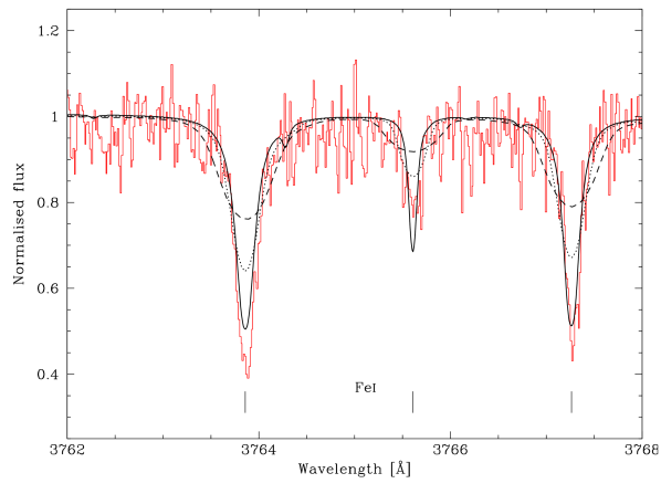
Figure 10: A close-up of three Fe I absorption lines in the white dwarf photosphere. Overplotted on the average spectrum are three TLUSTY/SYNSPEC models for $T_{\mathrm{WD}}=7500$ K, $\log g=7.75$, and the abundances listed in Table 3. The solid line shows a non-rotating white dwarf, the dotted line corresponds to $v\sin i=15$ km/s, and the dashed line to $v\sin i=30$ km/s.

We have used Echelle spectroscopy of the PCEB LTT 560 to derive precise system parameters. From the metal abundances in the white dwarf photosphere, we determined an accretion rate of $\sim 5\times 10^{-15}\mbox{$M_{\odot}$}\mathrm{yr^{-1}}$. Debes (2006) carried out a similar study of six white dwarf and main sequence binaries, both short-period (post-common envelope binaries, PCEBs) and wide binaries, and found accretion rates in the range $2\times 10^{-18}$ to $6\times 10^{-16}\mbox{$M_{\odot}$}\mathrm{yr^{-1}}$. Their study includes the system RR Cae, a white dwarf plus M-dwarf binary that resembles LTT 560 in many aspects. Both systems have nearly identical white dwarf masses and similar companion star masses, but the orbital period of RR Cae is nearly double that of LTT 560. Debes (2006) determined an accretion rate of $4\times 10^{-16}\mbox{$M_{\odot}$}\mathrm{yr^{-1}}$ for RR Cae, and inferred, assuming a spherically symmetric wind and Bondi-Hoyle type accretion, a wind mass-loss rate of $\dot{M}_{\mathrm{dM}}=6\times 10^{-15}\,\mathrm{M_{\odot}\,yr^{-1}}$ for the companion star. Taking the Bondi-Hoyle scenario at face value, $\dot{M}_{\mathrm{acc}}\propto 1/R^{2}$, where $R$ is taken as the distance between the white dwarf and the M dwarf. For an equally large wind mass-loss rate, the accretion rate in LTT 560 would be about three times higher than in RR Cae, which is only a factor of about three below the accretion rate that we estimated from the photospheric abundances. Considering all the uncertainties involved in estimating the accretion rate and mass-loss rate, RR Cae and LTT 560 appear to behave rather similar, and we speculate that it is the higher accretion rate in LTT 560 that is responsible for the chromosphere/corona around the white dwarf that we observe in H$\alpha$.

The accretion luminosity implied by $\dot{M}_{\mathrm{acc}}\simeq 5\times 10^{-15}\mbox{$M_{\odot}$}\mathrm{yr^{-1}}$ is $L\simeq 1.8\times 10^{28}\mathrm{erg\,s^{-1}}$. Integrating the H$\alpha$ flux, we find that $F(\mathrm{H}\alpha)\simeq 1.0\times 10^{-15}\mathrm{erg\,cm^{-2}\,s^{-1}}$, or, adopting $d=33$ pc (Paper I), $L(\mathrm{H}\alpha)\simeq 1.3\times 10^{26}\mathrm{erg\,s^{-1}}$, i.e. it is clear that the accretion-heated layer of the white dwarf must cool through additional emission mechanisms. In Paper I, we discussed how identifying LTT 560 with a nearby faint ROSAT PSPC source would imply an X-ray luminosity of $\sim 6\times 10^{27}\mathrm{erg\,s^{-1}}$, which is comparable to the predicted accretion luminosity. A deep X-ray observation would be desirable to confirm the association of LTT 560 with the ROSAT X-ray source and to establish more accurately the flux and spectral shape of the X-ray emission.

The nearly identical $\gamma$ velocities of both the white dwarf’s H$\alpha$ emission and the photospheric metal absorption lines suggest that they originate in the same region. However, because of the uncertainties involved we cannot exclude that the H$\alpha$ emission is produced somewhat above the white dwarf’s photosphere. For a “worst case scenario”, we calculate the largest possible difference within the 3$\sigma$ uncertainties as

$$\Delta\gamma=\gamma_{\mathrm{WD,metal}}+3\sigma_{\mathrm{metal}}-(\gamma_{\mathrm{WD,H\alpha}}-3\sigma_{\mathrm{H\alpha}})=2.15\leavevmode\nobreak\ \mathrm{km\leavevmode\nobreak\ s^{-1}}.$$

Since the white dwarf radius is given by $R_{\mathrm{WD}}=0.636\leavevmode\nobreak\ M_{\mathrm{WD}}/v_{\mathrm{gr}}$ for $M$ and $R$ in solar units and $v_{\mathrm{gr}}$ in $\mathrm{km\leavevmode\nobreak\ s^{-1}}$, $\Delta\gamma$ translates into $0.11R_{\mathrm{WD}}$. The H$\alpha$ emission could thus in principle originate in a region up to $\sim$1000 km above the photosphere. This still practically excludes a “strong” shock as the mechanism behind the emission, because the associated shock height is inversely correlated with the mass-transfer rate (e.g., Eq.14 in Fischer & Beuermann, 2001), which for LTT 560 is two orders of magnitude below that of even the low-accretion-rate polars (Schwope et al., 2002). It appears more likely that the emission line is produced by heat deposited by the accretion resulting in a temperature reversal shortly above the white dwarf photosphere. However, a detailed treatment of the physics involved is beyond the scope of this paper.

The narrow metal lines allow us to place a limit on the rotation rate of the white dwarf. Fig. 10 shows a close-up of three Fe I lines, along with models for $v\sin i=0$, 15, and 30 km/s, and suggests that the white dwarf in LTT 560 is a very slow ($\la 15$ km/s) rotator, similar to the majority of single white dwarfs (Koester et al., 1998; Karl et al., 2005; Berger et al., 2005). This is an interesting result, as it suggests that the evolution of angular momentum of white dwarfs in PCEBs is similar to that of field white dwarfs, with current theories requiring magnetic torques to explain the observed low rotation rates (e.g. Suijs et al., 2008).

The data sets used in Paper I and the present one show the occurrence of flares, indicating that there is an active secondary star in the system. Roche tomography shows an asymmetric surface brightness distribution, which we interpret as the presence of star spots (Fig. 9). These high latitude and/or polar spots are very common in single active stars (e.g., Strassmeier et al., 2003), and have also been observed on donor stars of CVs (Watson et al., 2006, 2007), as well as in the pre-CV V471 Tau (Hussain et al., 2006). The models of Granzer et al. (2000) suggest that star-spots emerge preferentially from the flux tube close to the equator of the star and are dragged by the Coriolis force to the pole of the star. Thus, high latitude and polar spots should be a common feature on rapid rotators, such as close binaries. However, we caution that these models are only valid for stars in the range $0.4\leavevmode\nobreak\ M_{\odot}\leq M\leq 1.7\leavevmode\nobreak\ M_{\odot}$ that contain a radiative core and a convective shell, and in LTT 560 the M5–6V secondary with a mass $M_{\mathrm{MS}}=0.14\leavevmode\nobreak\ M_{\odot}$ is well below this range and can be expected to be fully convective.

In addition to the high latitude features, we also observe that the inner face of the star in our model (the one facing the primary) is slightly darker than its backside. The low latitude star-spots populating the region around L1 appear to be another common feature in the tidally distorted late-type secondaries of close binaries (Watson et al., 2006, 2007; Hussain et al., 2006). It has been suggested by Holzwarth & Schüssler (2003) that tidal interaction may force spots to appear at preferred locations. King & Cannizzo (1998) find the appearance of such spots at L1 to be the probable mechanism behind the low brightness states and mass-transfer variations in CVs. As Watson et al. (2007) point out, a similar effect to that of star spots at L1 can be achieved by irradiation from the white dwarf primary, although the low temperature of the white dwarf ($T_{\mathrm{WD}}=7500\leavevmode\nobreak\ \mathrm{K}$; Paper I, ) indicates that this effect will be small if important at all.

What kind of future awaits LTT 560? Following Schreiber & Gänsicke (2003), we calculate the period $P_{\mathrm{sd}}$ at which the system becomes semi-detached as

$$P_{\mathrm{sd}}=2\pi\left(\frac{R_{\mathrm{MS}}^{3}}{G\leavevmode\nobreak\ M_{\mathrm{MS}}\leavevmode\nobreak\ (1+q^{-1})(R_{L}/a)^{3}}\right)^{\frac{1}{2}},$$ (4)

taken from Ritter (1986), with the approximation of Eggleton (1983)

$$R_{L}/a=\frac{0.49\leavevmode\nobreak\ q^{\frac{2}{3}}}{0.6\leavevmode\nobreak\ q^{\frac{2}{3}}+\ln(1+q)^{\frac{1}{3}}}.$$ (5)

With the parameters given in Table 2 (taking the average of the He- and the CO-configuration) and the secondary’s radius estimated from the RT, we find that $P_{\mathrm{sd}}=1.52^{+0.85}_{-0.43}\leavevmode\nobreak\ \mathrm{h}$. The large uncertainty here is dominated by our insufficient knowledge of $R_{\mathrm{MS}}$. Modelling the light curve of a photometric time-series data set of LTT 560 of high S/N would be desirable to improve the accuracy. Determining the distance to the system via a parallax measurement would similarly yield the absolute luminosities of the stellar components, thus provide independent access to both $R_{\mathrm{MS}}$ and $R_{\mathrm{WD}}$ and the associated parameters. Nevertheless, a $P_{\mathrm{sd}}$ below the period gap is consistent with the M5–6V spectral type of the secondary star (Beuermann et al., 1998; Smith & Dhillon, 1998). Since it can be assumed that the secondary is fully convective, we use Eq.8 from Schreiber & Gänsicke (2003) for angular momentum loss dominated by gravitational radiation to calculate the time it will take LTT 560 to start mass transfer via Roche-lobe overflow to $\sim$3.5 Gyrs. This is much less than the Hubble time, thus LTT 560 can be regarded as representative of the progenitors of todays CVs. Since the system contains a non-magnetic white dwarf and the mass ratio $q<0.33$, it is likely that the future CV LTT 560 will belong to the SU UMa subclass of dwarf novae.