On Consensus under Polynomial Protocols

Abstract

In this paper we explore the possibility of using computational algebraic methods to analyze a class of consensus protocols. We state some necessary conditions for convergence under consensus protocols that are polynomials.

1 Introduction

Consensus among agents is an important problem in multi-agent systems and congestion/flow control in communication networks. We formulate the problem as follows.

Consensus protocol is an ordered set of functions $(f_{1},f_{2},\ldots,f_{N})$, where $f_{i}:\mathbb{R}^{N}\longrightarrow\mathbb{R},\;i=1,\ldots,N$. We consider the following first order consensus dynamics among $n$ agents under this protocol

$$\dot{x}_{i}=f_{i}(x_{1},x_{2},\ldots,x_{N})\>\>\>i=1,\ldots,N.$$ (1)

Here $x_{1},x_{2},\ldots,x_{N}$ are the states of agents, the initial values of which are assumed to be known to the respective agents. The problem of interest is to determine whether the system of equations in (1) attains a consensus. Consensus is an equilibrium at which $x_{1}=x_{2}=\ldots=x_{N}$. In other words, we are interested to know whether there exist an $\alpha\in\mathbb{R}$ such that when $\mathbf{x}=\mathbf{x}_{e}$, where $\mathbf{x}=(x_{1},x_{2},\ldots,x_{N})$, and $\mathbf{x}_{e}$ is of the form $\mathbf{x}_{e}=(1,1,\ldots,1)\alpha$, we have $f_{i}(\mathbf{x}_{e})=0,i=1,\ldots,N,$ and starting from an arbitrary $\mathbf{x}$, the system (1) will converge to an equilibrium solution $\mathbf{x}_{e}$. Equation 1 can be written compactly as

$$\dot{\mathbf{x}}=\mathbf{f}(\mathbf{x}).$$ (2)

where $\mathbf{f}=(f_{1},f_{2},\ldots,f_{N})$. Here $\mathbf{f}$, the ordered $N\text{-tuple}$, is the consensus protocol and we are interested in protocols which will take the dynamical system (1) to consensus.

It is possible to associate a graph with every dynamical system of the form (1). Let $\mathcal{G}=(\mathcal{V},\mathcal{E})$ be a such graph with vertices $\mathcal{V}$ and edges $\mathcal{E}$. Then $\mathcal{V}=\{1,2,\ldots,N\}$ and a directed edge $e_{ij}=(i,j)$ from node $i$ to node $j$ belongs to $\mathcal{E}$ if $f_{j}$ is a function of $x_{i}$. If $f_{j}$ is a function of $x_{i}$, we say that $x_{i}$ belongs to the support of $f_{j}$, that is, $x_{i}\in supp(f_{j})$. Following Stigler [1], we call the graph $\mathcal{G}$ the dependency graph of (1). The neighbors of an agent/node $x_{i}$ are all those nodes which are in the support of $f_{i}$. Thus, the set of all neighbors of a node $i$ is

$$\mathcal{N}_{i}=\{j:e_{ji}\in\mathcal{E}\}.$$ (3)

The most widely analyzed protocol for consensus [2] is a linear protocol of form

$$\dot{x}_{i}=\sum_{j\in\mathcal{N}_{i}}(x_{j}-x_{i}),\quad i=1,\ldots,N.$$ (4)

The adjacency matrix, $A=[a_{ij}]$, associated with a graph $\mathcal{G}=(\mathcal{V},\mathcal{E})$ is defined as

$$a_{ij}=\left\{\begin{array}[]{ll}1&\text{if }e_{ij}\in\mathcal{E}\\ 0&\text{otherwise.}\end{array}\right.$$

A diagonal matrix called the degree matrix, $D=[d_{ii}]$, is defined as $d_{ii}=$ number of edges directed towards $x_{i}$, which is equal to ${\sum_{j=1}^{N}a_{ij}}$. The graph Laplacian, $L$, is defined as $L=D-A$. Using the definition of graph Laplacian, we can rewrite (4) as

$$\dot{\mathbf{x}}=-L\mathbf{x}$$ (5)

There is a great amount of literature on consensus under linear protocols. The assignment of a graph structure to the problem makes the problem amenable to application of tools from algebraic graph theory like graph Laplacian [3], stochasticity of nonnegative adjacency matrices [4], etc. to analyze the consensus in system given by (4) or a normalized form of it. However, these methods for analyzing stability and convergence to consensus of the system of equations may not be useful for nonlinear protocols.

There has been a few papers, in consensus literature, addressing consensus under nonlinear protocols. Olfati-Saber and Murray [3] considers consensus under a nonlinear protocol of form

$$\dot{x}_{i}=\sum_{j\in\mathcal{N}_{i}}h_{i}(x_{j}-x_{i}),\quad i=1,\ldots,n$$ (6)

where $h_{i},i=1,\ldots,n$ are functions which are uneven, locally Lipschitz, and strictly increasing.

Liu and Chen [5] extends this to protocols of form

$$\dot{x}_{i}=\sum_{j\in\mathcal{N}_{i}}\left(h(x_{j})-h(x_{i})\right),\quad i=1,\ldots,N$$ (7)

where $h$ is assumed to be an increasing function. However, this protocol demands that $h$ be same for all agents.

Moreau [6] proves the convergence of consensus protocol under the assumption that the protocol is such that, in the discretized version of it, the updated value of a node is a strict convex combination of current values of the node and its neighbors . This implies that the continuous time protocol of the form

$$\dot{x}_{i}=\sum_{j\in\mathcal{N}_{i}}h_{j}(\mathbf{x})(x_{j}-x_{i}),\quad i=1,\ldots,N$$ (8)

will achieve consensus.

This paper we pose problem of consensus under polynomial protocols in the framework of computational algebra and give necessary conditions for the convergence. This paper is organized as follows. In § 2 we give preliminary observations on polynomial consensus and review basic background in computational algebra that is required. We present main results in § 3 and give concluding remarks in § 4

2 Preliminary Observations and Basic Computational Algebra

2.1 Preliminary Observations

We give few necessary conditions for convergence to a consensus under polynomial protocols, using the tools and language of algebraic geometry. It is clear that for a consensus to be achieved, the protocol $\mathbf{f}$ should use all the nodal values. A consensus is not achieved, except for some particular initial conditions, if values of one or mode nodes are not used in the dynamics (2). This leads us to the following proposition.

Proposition 1

If the system $\dot{x}_{i}=f_{i},i=1,\ldots,N$, achieves consensus, then for all $j\in\{i,\ldots,N\}$, there exists $i\in\{i,\ldots,N\}$ such that $x_{j}\in supp(f_{i})$.

The proposition asserts that the dependency graph of a protocol that achieve consensus should not have any isolated nodes.

Also, if more than one nodal values are not being updated, it is not possible to arrive at a consensus in general. However, there might exist a few particular initial conditions for which a consensus on nodal values is reached. For example, the initial values of the nodes whose values are not being updated are equal and equal to the consensus value achieved by other nodes. However, this is an exception rather than a rule. Therefore, we have the following necessary condition.

Proposition 2

If more than one $f_{i}$ are zero polynomials, then the system $\dot{x}_{i}=f_{i},i=1,\ldots,N$, will not achieve consensus.

A result from theory of linear consensus protocols states that a consensus is not achieved if the underlying graph does not have a directed spanning tree [7]. Proposition 2 has the same flavor.

From here onwards when we say that a protocol $\mathbf{f}$ satisfies the conditions for Propositions 1 and 2, we mean that the protocol involves all the nodal values and at most one of the polynomials in $\mathbf{f}$ is a zero polynomial. And, whenever one of the polynomials is a zero polynomial, by the set $\{f_{1},\ldots,f_{N}\}$ we mean the set without the zero polynomial.

If the system of equations in Eq. (2) leads to a consensus, then we have $\dot{\mathbf{x}}=0$, which implies $\mathbf{f}(\mathbf{x})=0$, asymptotically. The equilibrium points of the system of equations in Eq. (2) are the ‘roots’ of the set of polynomial equations $\mathbf{f}(\mathbf{x})=0$. Now we need some notions of algebraic geometry and Gröbner bases.

2.2 Basics of Algebraic Geometry and Gröbner bases

Throughout this paper, $\Bbbk$ represents a field (e.g., $\mathbb{R}$, $\mathbb{C}$). Set of all monomials in indeterminates $x_{1},\ldots,x_{N}$ is denoted by ${\mathbb{Z}}_{\geq 0}^{n}$ and set of all polynomials in indeterminates $x_{1},\ldots,x_{N}$ with coefficients in $\Bbbk$ is denoted by $\Bbbk[x_{1},\ldots,x_{N}]$. Let $f_{1},\ldots,f_{s}\in\Bbbk[x_{1},\ldots,x_{N}]$. We use the notation $\mathcal{V}(f_{1},\ldots,f_{s})=V$ to represent the varieties, where

$$V=\{(c_{1},\ldots c_{n})\in\Bbbk^{N}:f_{i}(c_{1},\ldots c_{N})=0,1\leq i\leq s\}\enspace.$$

$V$ is uniquely determined by the ideal generated by $f_{1},\ldots,f_{s}$. This ideal is denoted by ${\langle f_{1},\ldots,f_{s}\rangle}$ and hence we have

$${\mathcal{V}}(f_{1},\ldots,f_{s})={\mathcal{V}}({\langle f_{1},\ldots,f_{s}\rangle})\enspace.$$

The set of equilibrium points of most of the consensus protocols contain the subspace $x_{1}=\cdots=x_{N}$. Let us call this subspace where states of all agents are equal as $\mathcal{S}$. If a protocol $\mathbf{f}$ leads to consensus, then it should have at least one equilibrium point belonging to the subspace $\mathcal{S}$. Thus we get a necessary condition for convergence of Eq. (2) as follows. If Eq. (2) converges, then $\mathcal{S}\cap\mathcal{V}(\mathbf{f})$ is nonempty. Geometrically, the subspace $\mathcal{S}\subset\Bbbk^{N}$ is a solution to set of equations

$$\mathbf{s}=\{x_{1}-x_{2},x_{2}-x_{3},\ldots,x_{N-1}-x_{N}\}$$ (9)

In the language of algebraic geometry, $\mathcal{S}$ is the variety of $\mathbf{s}$, that is, $\mathcal{S}=\mathcal{V}(\mathbf{s}).$ Therefore, a consensus would imply $\mathcal{V}(\mathbf{s})\cap\mathcal{V}(\mathbf{f})$ is non-empty.

Let ${J}$ be the ideal generated by set of polynomials $\mathbf{s}$ describing the subspace $\mathcal{S}$ as described before. It is easy to see that the affine variety of the set of polynomials $\mathbf{s}$ is equal to the affine variety of the ideal ${J}$ generated by them [8], that is, $\mathcal{V}({J})=\mathcal{V}(\mathbf{s})=\mathcal{S}$.

Since $\mathcal{S}$ is an irreducible variety (cannot be written as the union of non-empty varieties), the ideal ${J}$ is prime [8]. Since $J$ is prime, the radical ideal of ${J}$ is itself. Now, by Hilbert’s Strong Nullstellansatz [8], the ideal $\mathcal{I}(\mathcal{S})$, the ideal of all polynomials that vanishes at every point on $\mathcal{S}$, is $J$.

Throughout this article, we will be using some results from algebraic geometry. These will be given as propositions and theorems without proofs and we refer an interested reader for details to Cox et al. [8].

Theorem 2.1

[8] If $I$ and $J$ are ideals in $\Bbbk[x_{1},\ldots,x_{N}]$, then $\mathcal{V}(I+J)=\mathcal{V}(I)\cap\mathcal{V}(J)$.

Here, $I+J$ is defined as follows.

Definition 1

If $I$ and $J$ are ideals of ring $\Bbbk[x_{1},\ldots,x_{N}]$, then the sum of $I$ and $J$, denoted by $I+J$, is the set

$$I+J=\{f+g|f\in I\;\text{and}\;g\in J\}.$$

In fact, $I+J$ is the smallest ideal containing both $I$ and $J$ [8]. We have the following proposition.

Proposition 3

Let ${I}$ be the ideal generated by $\{f_{1},\ldots,f_{N}\},f_{i}\in\Bbbk[x_{1},\ldots,x_{N}]$, $i=1,\ldots,N$ and ${J}$ be the ideal $\langle x_{1}-x_{2},x_{2}-x_{3},\ldots,x_{N-1}-x_{N}\rangle$. Let $\mathcal{S}\subset\Bbbk^{N}$ be the subspace given as $\mathcal{S}=\{(x_{1},\ldots,x_{N})\in\Bbbk^{N}:x_{1}=x_{2}=\cdots=x_{N}\}$. Then, if the polynomial dynamical system $\dot{x}_{i}=f_{i},i=1,\ldots,N$ attains consensus, then $\mathcal{V}({I}+{J})$ is not empty and ${I}+{J}$ is a proper subset of $\Bbbk[x_{1},\ldots,x_{N}]$.

Proof

A necessary condition for consensus is that at least one of the stationary points of the system $\dot{x}_{i}=f_{i},i=1,\ldots,n$ should belong to $\mathcal{S}$. Set of stationary points or the invariant set of this system is the solution to set of polynomial equations $f_{1}=0,\ldots,f_{N}=0$ which is given by $\mathcal{V}(I)$. Thus the necessary condition demands that $\mathcal{V}(I)\cap\mathcal{S}$ is not empty. Since $\mathcal{S}$ is Zariski closed as $\mathcal{S}$ is the variety of ideal $\mathcal{J}$, we get $\mathcal{V}(I)\cap\mathcal{V}({J})\neq\emptyset$. This along with Theorem 2.1 gives that $\mathcal{V}({I}+{J})$ is not empty. Since $\mathcal{V}({I}+{J})$ is not empty, by Hilbert’s Weak Nullstellensatz [8], ${I}+{J}$ is proper ideal of $\Bbbk[x_{1},\ldots,x_{N}]$.

The statements on ideals can be checked by calculating their Gröbner bases which can be done using any symbolic package that supports algebraic geometric calculations, given the set of polynomials that generate the ideal. Now, we define a Gröbner basis.

Gröbner bases is a generalization of the division algorithm in a single variable case ($\Bbbk[x]$) to the multivariate case ($\Bbbk[x_{1},\ldots,x_{N}]$). Gröbner basis also generalizes Gaussian elimination in linear polynomials to nonlinear polynomials. For the multivariate division algorithm, we need the notion of monomial order.

Definition 2

A monomial order or term order on $k[x_{1},\ldots,x_{N}]$ is a relation $\prec$ on ${\mathbb{Z}}_{\geq 0}^{N}$ that satisfies following conditions (i) $\prec$ is a total ordering on ${\mathbb{Z}}_{\geq 0}^{N}$, (ii) if $\alpha\prec\beta$, for $\alpha,\beta\in{\mathbb{Z}}_{\geq 0}^{N}$ then for any $\gamma\in{\mathbb{Z}}_{\geq 0}^{N}$ it holds $\alpha+\gamma\prec\beta+\gamma$, and (iii) $\prec$ is a well-ordering on ${\mathbb{Z}}_{\geq 0}^{N}$.

Given such an ordering $\prec$, one can define the leading term of non-zero polynomial $f\in\Bbbk[x_{1},\ldots,x_{N}]$ as a term of $f$ (the coefficient times its monomial) whose monomial is maximal for $\prec$. We denote this leading term by $\text{LT}_{\prec}(f)$ and the corresponding monomial by $\text{LM}_{\prec}(f)$.

Definition 3

An ideal $\mathfrak{a}\subset\Bbbk[x_{1},\ldots,x_{N}]$ is said to be a monomial ideal if there is a set $A\subset{\mathbb{Z}}_{\geq 0}^{N}$, possibly infinite, such that $\mathfrak{a}=\langle x^{\alpha}:\alpha\in A\rangle$.

Given any ideal $\mathfrak{a}\subset\Bbbk[x_{1},\ldots,x_{N}]$, the ideal defined as $\langle\text{LM}_{\prec}(f):f\in\mathfrak{a}\rangle$ is a monomial ideal and is denoted by $\text{LM}_{\prec}(\mathfrak{a})$, which is known as leading monomial ideal of $\mathfrak{a}$. By Dickson’s lemma [8, p. 69], the ideal $\text{LM}_{\prec}(\mathfrak{a})$ is generated by a finite set of monomials. Dickson’s lemma and the multivariate division algorithm leads to a proof of Hilbert bases theorem which states that every polynomial ideal can be finitely generated, which further lead to a definition of Gröbner basis [8, § 2.5].

Definition 4

Fix a monomial order $\prec$ on $\Bbbk[x_{1},\ldots,x_{N}]$. A finite subset $G=\{g_{1},\ldots,g_{s}\}$ of an ideal $\mathfrak{a}\subset\Bbbk[x_{1},\ldots,x_{N}]$ is a Gröbner basis if and only if $\text{LM}_{\prec}(\mathfrak{a})$ $=$ $\langle\text{LM}_{\prec}(g_{1}),\ldots,$ $\text{LM}_{\prec}(g_{s})\rangle.$

Given a set of generators of an ideal, the Buchberger algorithm [10] can be used to compute a Gröbner basis of the ideal with respect to various term orders. The algorithm and its variants are implemented in most symbolic computation programs. Note that a Gröbner basis is not unique, but one can transform it to a reduced Gröbner basis which is unique for every ideal in $\Bbbk[x_{1},\ldots,x_{N}]$. In the sequel, when we say ‘the Gröbner basis’, we mean the reduced Gröbner basis. The Buchberger algorithm provides a common generalization of the Euclidean division algorithm and the Gaussian elimination algorithm to multivariate polynomial rings.

3 Consensus under polynomial protocols: Necessary conditions

Now, an equivalent statement of Proposition 3 in terms of Gröbner basis can be given as follows.

Corollary 1

If ${G}$ is a Gröbner basis of ${I}+{J}$ where $I$ and $J$ are as defined in Proposition 3, then the affine variety of ${G}$ is not empty and the ideal generated by ${G}$ is a proper ideal of $\Bbbk[x_{1},\ldots,x_{N}]$.

The above condition will always be satisfied if none of the $f_{i},i=1,\ldots,N$, has a constant term, as then, $\mathbf{x}=\mathbf{0}$ is a common solution of polynomials in both $I$ and $J$. We call this the trivial consensus where a consensus occurs if the initial conditions on all the nodes are simultaneously zeros. Similarly, consensus occurs for other special initial cases too. Since the conditions of Proposition 3 also holds for protocols that can achieve trivial consensus also, it is a weak result.

From Proposition 3 we have that, to show that a system does not attain consensus, it is enough to show that $I+J$ is the entire polynomial ring $\Bbbk[x_{1},\ldots,x_{N}]$, or equivalently by Hilbert’s Weak Nullstellansatz, the Gröbner basis of ideal $I+J$ is $1$ (since $1$ generates the whole ring $\Bbbk[x_{1},\ldots,x_{N}]$ which has an empty variety). For this, we need a way to calculate the ideal $I+J$ given $I$ and $J$, which the following proposition gives.

Proposition 4

[8]If $I=\langle f_{1},\ldots,f_{r}\rangle$ and $J=\langle g_{1},\ldots,g_{s}\rangle$, then $I+J=\langle f_{1},\ldots,f_{r},g_{1},\ldots,g_{s}\rangle$.

Thus to check the Proposition 3, given $\langle\mathbf{f}\rangle$, the ideal generated by protocols, and $\langle\mathbf{s}\rangle$, the ideal the variety of which is $\mathcal{S}$, we need to calculate the variety of ideal $\langle\mathbf{f}\rangle+\langle\mathbf{s}\rangle$ which by Proposition 4 is equal to the variety of $\langle\mathbf{f},\mathbf{s}\rangle$. Since a Gröbner basis of $\langle\mathbf{f},\mathbf{s}\rangle$ has the same variety as that of $\langle\mathbf{f},\mathbf{s}\rangle$, it is enough to calculate the Gröbner basis of $\langle\mathbf{f},\mathbf{s}\rangle$ and look at its variety. This can be done using any software that support computation of Gröbner basis. For the examples given in this chapter, we use Mathematica.

Example 1

We consider a nonlinear protocol as follows.

$$\begin{array}[]{rrr}\dot{x}_{1}=x_{1}+x_{2}+1,&\dot{x}_{2}=x_{1}+x_{3}+3,&\dot{x}_{3}=x_{2}-x_{3}.\end{array}$$

$\boldsymbol{\text{GroebnerBasis}[\{\{x_{1}+x_{2}+1,x_{1}+x_{3}+3,x_{2}-x_{3}\},}\boldsymbol{\{x_{1}-x_{2},x_{2}-x_{3}\}\}]}$

$\{1\}$

For the system in Eq. (1), a consensus is achieved if there exists an $\alpha\in\mathbb{R}$ such that $x_{1}=x_{2}=\cdots=x_{N}=\alpha$ is an equilibrium point. However, systems for which $x_{1}=x_{2}=\cdots=x_{N}=\alpha$ is an equilibrium point for all $\alpha\in\mathbb{R}$ are of particular interest in the consensus community. Therefore, in the rest of the paper, we consider only such protocols. The necessary condition as given in Proposition 3 then amounts to $\mathcal{V}(J)\subseteq\mathcal{V}(I)$, where $I=\langle f_{1},f_{2},\ldots,f_{N}\rangle$ and $J=\langle x_{2}-x_{1},x_{3}-x_{2},\ldots,x_{N-1}-x_{N}\rangle$.

A consensus cannot be achieved over a graph that is disconnected. Thus a necessary condition for a consensus to occur under a protocol is that its dependency graph should be connected. In the case of a linear protocol with a dependency graph that is directed, it should be strongly connected (or at least should have a directed spanning tree) for consensus to occur [7]. A result from algebraic graph theory states that if a directed graph is strongly connected, then for a linear consensus protocol the graph Laplacian matrix associated with it is irreducible [11]. This essentially means that by a permutation or an automorphism of the variables, the associated graph Laplacian can be made to be of a block diagonal form. The number of blocks are equal to the number of disconnected components of the graph [7]. Given a protocol $\mathbf{f}=\{f_{1},\ldots,f_{N}\}$, its dependency graph $\mathcal{G}=(\mathcal{V},\mathcal{E})$ can be found. It is possible to characterize the properties of this graph by defining the following relation.

Definition 5

Given two nodes $i,j\in\mathcal{V}$, we say $i\prec_{p}j$ if there exists a path from node $j$ to node $i$. If $i\prec_{p}j$ and $j\prec_{p}i$, then nodes $i$ and $j$ are path-equivalent and we denote this by $i\sim_{p}j$.

The relation $\prec_{p}$ is anti-symmetric since if $i\prec_{p}j$ and $j\prec_{p}i$, then $i\sim_{p}j$. It is transitive. The above relation is reflexive and hence a partial order if the dependency graph contains self-loops.

We have the following results that are immediate from the definition of the order relation $\prec_{p}$.

Proposition 5

Let $\mathcal{G}=(\mathcal{V},\mathcal{E})$ be graph with $\mathcal{V}=\{1,\ldots,N\}$. Let $\text{Maximal}_{\prec_{p}}\mathcal{V}$ denote the set of maximal elements in $\mathcal{V}$ under the order relation $\prec_{p}$. Then,

1. The graph $\mathcal{G}$ is strongly connected if and only if $\text{Maximal}_{\prec_{p}}\mathcal{V}=\mathcal{V}$

2. The graph $\mathcal{G}$ has a directed spanning tree if and only if
   $\#\left(\text{Maximal}_{\prec_{p}}\mathcal{V}/\sim_{p}\right)=1$

where $\#$ denotes the cardinality of a set.

The necessary and sufficient condition for achieving a consensus under linear protocol over a graph is the existence of a directed spanning tree [7]. In fact, the existence of a directed spanning tree is a necessary condition not only for the linear consensus protocol but also for any protocol that achieves consensus over a graph.

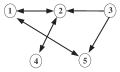
Figure 1: Dependency graph with a directed spanning tree rooted at node 3.

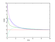
Figure 2: Consensus under protocol in Eq. (10).

Example 2

The linear protocol

$$\dot{x}_{i}=\sum_{j\in\mathcal{N}_{i}}x_{j}-{|\mathcal{N}_{i}|}x_{i}$$ (10)

applied to dependency graph given in Fig. 1 is

$$\begin{array}[]{lllll}\dot{x}_{1}=x_{2}+x_{5}-2x_{1},&\dot{x}_{2}=x_{1}+x_{3}+x_{4}-3x_{2},&\dot{x}_{3}=0,&\\ \dot{x}_{4}=x_{2}-x_{4},&\dot{x}_{5}=x_{1}+x_{3}-2x_{5}.\end{array}$$

Convergence to consensus under this protocol is given in Fig. 2.

Example 3

We now consider consensus under a nonlinear protocol

$$\dot{x}_{i}=\sum_{j\in\mathcal{N}_{i}}x_{j}^{2}-{|\mathcal{N}_{i}|}x_{i}^{2}$$ (11)

for the dependency graph in Fig. 1

$$\begin{array}[]{lllll}\dot{x}_{1}=x_{2}^{2}+x_{5}^{2}-2x_{1}^{2},&\dot{x}_{2}=x_{1}^{2}+x_{3}^{2}+x_{4}^{2}-3x_{2}^{2},&\dot{x}_{3}=0,\\ \dot{x}_{4}=x_{2}^{2}-x_{4}^{2},&\dot{x}_{5}=x_{1}^{2}+x_{3}^{2}-2x_{5}^{2}.\end{array}$$

Figure 3 shows the convergence to consensus of this protocol.

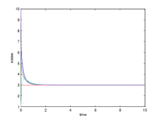
Figure 3: Consensus under protocol in Eq. (11).

Example 4

The third protocol considered earlier is

$$\dot{x}_{i}=\prod_{j\in\mathcal{N}_{i}}x_{j}-x_{i}^{|\mathcal{N}_{i}|}$$ (12)

Applied to dependency graph of Fig. 1, we get

$$\begin{array}[]{rrrrr}\dot{x}_{1}=x_{2}x_{5}-x_{1}^{2},&\dot{x}_{2}=x_{1}x_{3}x_{4}-x_{2}^{3},&\dot{x}_{3}=0,&\dot{x}_{4}=x_{2}-x_{4},&\dot{x}_{5}=x_{1}x_{3}-x_{5}^{2}.\end{array}$$

Figure 4 shows that this protocol leads to consensus.

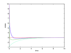
Figure 4: Consensus under protocol in Eq. (12).

Examples 2–4 give protocols all of which had a dependency graph that is not strongly connected but still achieve consensus. This shows that the dependency graph of a protocol being strongly connected is not a necessary condition for consensus to occur.

Using the elimination theorem from algebraic geometry, we can get a result that enables us to determine whether the dependency graph of a polynomial protocol has a directed spanning tree. To state the elimination theorem, we need concepts of elimination order and elimination ideal as defined below.

Definition 6

Consider $\Bbbk[x_{1},\ldots,x_{n},y_{1},\ldots,y_{m}]$ a polynomial ring in indeterminates $x_{1},\ldots,x_{n}$, $y_{1},\ldots,y_{m}$. Let $\prec_{x}$ and $\prec_{y}$ be monomial orderings on $x$ and $y$ variables respectively. Define an ordering relation $\prec_{[\{x\}\succ\{y\}]}$ on ${\mathbb{Z}}_{\geq 0}^{n+m}$ (i.e set of all monomials in indeterminates $x_{1},\ldots,x_{n},y_{1},\ldots,y_{m}$) as follows:

$$x^{a}y^{b}\prec_{[\{x\}\succ\{y\}]}x^{c}y^{d}\Longleftrightarrow\left\{\begin{array}[]{l}a\prec_{x}c\\ \mathrm{or}\\ a=c\>\>\mathrm{and}\>\>b\prec_{y}d\end{array}\right.\enspace,$$

where $a,c\in{\mathbb{Z}}_{\geq 0}^{n}$ and $b,d\in{\mathbb{Z}}_{\geq 0}^{m}$. The term order $\prec_{[\{x\}\succ\{y\}]}$ is called elimination order with the $x$ variables larger than the $y$ variables (which is indeed a term order).

Definition 7

Given $I=\langle f_{1},\ldots,f_{s}\rangle\subset\Bbbk[x_{1},\ldots,x_{N}]$ the $l$-th elimination ideal $I_{l}$ is the ideal of $\Bbbk[x_{l+1},\ldots,x_{N}]$ defined by $I_{l}=I\cap\Bbbk[x_{l+1},\ldots,x_{N}]$

Now, we sate the elimination theorem.

Theorem 3.1

[8] Let $I\subset\Bbbk[x_{1},\ldots,x_{N}]$ be an ideal and let $G$ be a Gröbner Basis of $I$ with respect to an elimination order where $\{x_{1},x_{2},\ldots,x_{l}\}\succ\{x_{l+1},\ldots,x_{N}\}$ for every $0\leq l\leq N$. Then the set

$$G_{l}=G\cap\Bbbk[x_{l+1},\ldots,x_{N}]$$

is a Gröbner Basis of the $l$-th elimination ideal $I_{l}$.

If the dependency graph of a linear consensus protocol contains a directed spanning tree, then the corresponding Laplacian matrix, $L$, will be of rank $N-1$ [7]. This means that it is possible to eliminate $N-2$ variables from the protocol $L\mathbf{x}$ using Gaussian elimination. Since the elimination in the multivariate polynomial case is the generalization of the Gaussian elimination, we expect this nice property of being able to eliminate $N-2$ variables in the linear protocol case to carry over to polynomial protocols that attain consensus.

Theorem 3.2

Let $f_{i}\in\Bbbk[x_{1},\ldots,x_{N}],$ $i=1,\ldots,N.$ Let $I=\langle f_{1},f_{2},\ldots,f_{N}\rangle$ be such that $\mathcal{V}(J)\subseteq\mathcal{V}(I)$ for $J=\langle x_{2}-x_{1},x_{3}-x_{,}\ldots,x_{N-1}-x_{N}\rangle$. If the system $\dot{x}_{i}=f_{i},i=1,\ldots,N$ attains consensus, then the $(N-2)$-th elimination ideal of $\langle f_{1},\ldots,f_{N}\rangle$ is not empty under any elimination order with $\{x_{\sigma(1)},\ldots,x_{\sigma(N-2)}\}\prec\{x_{\sigma(N-1)},x_{\sigma(N)}\}$ where $\sigma$ belongs to the set of every possible permutation of $\{1,\ldots,N\}$.

This follows from the fact that a consensus is achieved only if the dependency graph has a directed spanning tree. We illustrate this through the following example.

Example 5

Consider a polynomial protocol given as

$$\begin{array}[]{r r r r}\dot{x}_{1}=x_{2}-x_{1},&\dot{x}_{2}=x_{1}-x_{2},&\dot{x}_{3}=0,&\dot{x}_{4}=x_{1}x_{2}x_{3}-x_{4}^{3}.\end{array}$$

The corresponding dependency graph is shown in Fig. 5. This dependency graph does not have a directed spanning tree and thus will not attain a consensus. Thus by Theorem 3.2, there should exist an elimination order under which it may not possible to eliminate 2 variables from the Gröbner Basis of $\{x_{2}-x_{1},x_{1}-x_{2},x_{1}x_{2}x_{3}-x_{4}^{3}\}$. If we try to eliminate the highest two variables under the elimination order $\{x_{4},x_{3}\}\prec\{x_{2},x_{1}\}$, we get an empty set implying that the elimination is not possible.

$\boldsymbol{\text{GroebnerBasis}[\{x_{2}-x_{1},x_{1}-x_{2},x_{1}x_{2}x_{3}-x_{4}^{3}\},\{x_{4},x_{3}\},\{x_{2},x_{1}\}]}$

$\{\}$

Figure 5: Dependency graph of protocol in Example 5

It is possible to extend the result in Theorem 3.2, to the following.

Proposition 6

Let $\mathbf{f}=(f_{1},\ldots,f_{N})\in\Bbbk[x_{1},\ldots,x_{N}]^{N}$ be such that $\mathcal{V}(J)\subseteq\mathcal{V}(I)$ for $J=\langle x_{2}-x_{1},x_{3}-x2,\ldots,x_{N-1}-x_{N}\rangle$ and $I=\langle f_{1},f_{2},\ldots,f_{N}\rangle$. Let $l\in\mathbb{N}$ be the smallest $l$ such that the $l$-th elimination ideal of $\langle f_{1},\ldots,f_{N}\rangle$ is empty under an elimination order with $\{x_{i_{1}},\cdots,x_{i_{l}}\}\succ\{x_{i_{l+1}},\ldots,x_{i_{N}}\}$ where $\{i_{1},\ldots,i_{N}\}$ is a permutation of $\{1,\ldots,N\}$. Then, $\#\left(\text{Maximal}_{\prec_{p}}\mathcal{V}/\sim_{p}\right)=N-l$.

For Example 5, we have $N=4$, $l=2$, and from Fig. 5 we see that

$$\#\left(\text{Maximal}_{\prec_{p}}\mathcal{V}/\sim_{p}\right)=2.$$

4 Concluding Remarks

We explored a novel way of looking at the consensus over networks–the algebraic geometric way–when the protocols are polynomials. We gave several necessary conditions for obtaining consensus under polynomial protocols. This enables one to comment on the convergence to consensus of a protocol by looking at the computed Gröbner Basis of the set of polynomials in the protocol. We also gave a sufficient condition for convergence under polynomial consensus. We conclude by remarking that algebraic geometry, if used properly, has sufficient powerful tools to analyze consensus under switching protocols and to design consensus protocols with desired behaviors.

References

- [1] B. Stigler, An algebraic approach to reverse engineering with an application to bio-chemical networks, Ph.D. thesis, Virginia Polytechnic Institute and State University, 2005.
- [2] R. Olfati-Saber, J. A. Fax, and R. M. Murray, “Consensus and cooperation in networked multi-agent systems,” Proc. IEEE, vol. 95, no. 1, pp. 215-233, Jan. 2007.
- [3] R. Olfati-Saber, and R. M. Murray, “Consensus protocols for networks of dynamic agents,” in Proc. 2003 Am. Control Conf., 2003, pp. 951-956.
- [4] A. Jadbabaie, J. Lin, and A. S. Morse, “Coordination of groups of mobile autonomous agents using nearest neighbor rules,” IEEE Trans. Autom. Control, vol. 48, no. 6, pp. 9881001, Jun. 2003.
- [5] X. Liu, and T. Chen, “Consensus Problems in Networks of Agents under Nonlinear Protocols with Directed Interaction Topology,” arXiv:0804.3628v1 [math.DS] 23 Apr 2008.
- [6] L. Moreau, “Stability of multi-agent systems with time-dependent communication links,” IEEE Trans. Autom. Control, vol. 50, no. 2, pp. 169182, Feb. 2005.
- [7] W. Ren, R. W. Beard, and E. Atkins, “Information Consensus in Multivehicle Cooperative Control: Collective Group Behavior through Local Interaction,” IEEE Control Systems Magazine, vol. 27, no. 2, pp. 71-82, Apr. 2007.
- [8] D. Cox, J. Little, and D. O’Shea, Ideals, varieties, and algorithms, Springer Verlag, New York, 1997.
- [9] W.W. Adams, and P. Loustaunau, An Introduction to Gröbner Basis, American Mathematical Society, Providence, 1994.
- [10] B. Buchberger, and Gröbner, “An algorithmic method in polynomial ideal theory,” In Multidimensional Systems Theory, (Ed.) N. K. Bose, D. Reidel, 1985.
- [11] C. Godsil, and G. Royle, Algebraic Graph Theory, Graduate Texts in Mathematics, 207, Springer-Verlag, New York, 2001.
- [12] G. L. Calandrini, E. E. Paolini, and J. L. Moiola, “Groebner bases for designing dynamical systems,” Latin American Applied Research, vol. 33, pp. 427–434, 2003.