Thermoelectric transport of mesoscopic conductors coupled to voltage and thermal probes

Abstract

We investigate basic properties of the thermopower (Seebeck coefficient) of phase-coherent conductors under the influence of dephasing and inelastic processes. Transport across the system is caused by a voltage bias or a thermal gradient applied between two terminals. Inelastic scattering is modeled with the aid of an additional probe acting as an ideal potentiometer and thermometer. We find that inelastic scattering reduces the conductor’s thermopower and, more unexpectedly, generates a magnetic-field asymmetry in the Seebeck coefficient. The latter effect is shown to be a higher-order effect in the Sommerfeld expansion. We discuss our result using two illustrative examples. First, we consider a generic mesoscopic system described within random matrix theory and demonstrate that thermopower fluctuations disappear quickly as the number of probe modes increases. Second, the asymmetry is explicitly calculated in the quantum limit of a ballistic microjunction. We find that asymmetric scattering strongly enhances the effect and discuss its dependence on temperature and Fermi energy.

Introduction. Recent advances in heat measurements have enabled to envisage promising thermoelectric applications at the mesoscale. gia06 In particular, there have been a number of exciting proposals ranging from thermal analogs of electronic rectifiers ter02 and transistors wan07 to efficient converters of heat into electricity bel08 which can be shown to reach optimized configurations. san10 Of fundamental importance is the experimental verification of the carriers’ charge sign using thermopower techniques only. red07

Since these novel devices operate at the quantum regime of transport, it is of primary interest to investigate dephasing effects which may be detrimental to their performance. Additionally, energy flow at finite temperature is expected to be particularly sensitive to inelastic transitions inside the sample due, e.g., to coupling to phonons. This problem has been addressed only very recently. lei10 ; ent10

A convenient way to introduce dephasing and energy relaxation in a mesoscopic conductor is based on the voltage probe model. but86 A fictitious terminal is attached to the sample such that the net current flowing through the probe is set to zero. Hence, a carrier absorbed by the probe is reemitted into the conductor with an unrelated phase. The clear advantage of this approach lies on its simplicity and its independence of the microscopic details of the phase-randomizing processes. Therefore, universal properties of generic conductors can be investigated this way. bar95 ; bro97 The model has been recently applied to find the temperature and chemical potential profiles of an array of quantum dots. jac09

Including a third terminal acting as a dephasing probe requires to extend the scattering approach to the multiterminal case. For thermoelectric transport, this was achieved by Butcher. but90 Experimentally, there are already available data for paradigmatic mesoscopic systems such as two-terminal point contacts mol92 and chaotic cavities. god99 The multiterminal case, however, has been less explored. A very recent exception is Ref. mat11, where a voltage drop is generated transversally to a horizontal thermal gradient in a four-terminal setup with an asymmetric scatterer.

Here we investigate incoherent scattering effects on the thermopower (Seebeck coefficient $S$), defined at linear response as the ratio of voltage $\Delta V$ to temperature $\Delta\theta$ differences applied between two terminals (1 and 2 in Fig. 1) at vanishing current $I$,

$$S\equiv\left.\frac{\Delta V}{\Delta\theta}\right|_{I=0}\;,$$ (1)

in the presence of an attached probe (terminal 3 in Fig. 1) acting as an ideal potentiometer and thermometer. Quite generally, we find that $S$ decreases as compared to the case without probe and, strikingly, the presence of incoherent scattering due to the probe causes the development of a magnetic-field asymmetry in $S$. To illustrate our findings, we analyze (i) a mesoscopic conductor with generic properties (a chaotic cavity); and (ii) a ballistic wire in the quantum limit (a few propagating modes) with an asymmetric scatterer. In the latter case, we explicitly calculate the size of the magnetoasymmetry. This result is relevant in view of recent predictions that relate this asymmetry to efficiency limits of thermal devices in converting a temperature gradient into electrical work. ben11 ; sai11

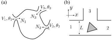
Figure 1: Sketches of (a) a chaotic cavity attached to voltage and thermal reservoirs and (b) a microjunction with an asymmetric scatterer coupled to a probe as a model of a quantum wire with incoherent scattering.

Model. We consider a mesoscopic conductor coupled to three terminals. Thermoelectric transport is described by the electric current, $I_{\alpha}$, and the heat current, $Q_{\alpha}$, flowing from terminal $\alpha=1,2,3$. In the linear response regime, the transport equations read:

$$I_{\alpha} =\sum_{\beta}G_{\alpha\beta}V_{\beta}+\sum_{\beta}L_{\alpha\beta}\theta_{\beta}\,,$$ (2)

$$Q_{\alpha} =\sum_{\beta}M_{\alpha\beta}V_{\beta}+\sum_{\beta}K_{\alpha\beta}\theta_{\beta}\,,$$ (3)

where $eV_{\alpha}=E_{F}-\mu_{\alpha}$ are voltage shifts away from the common Fermi energy $E_{F}$, with $\mu_{\alpha}$ the electrochemical potential of lead $\alpha$, while $\theta_{\alpha}=\theta-T_{\alpha}$ measures deviations of the reservoir temperature $T_{\alpha}$ from the common (bath) temperature $\theta$. The transport coefficients are expressed in terms of the transmission probability $T_{\alpha\beta}$:

$$G_{\alpha\beta} =-g_{V}\int\!dE\,(N_{\alpha}\,\delta_{\alpha\beta}-T_{\alpha\beta})f_{0}^{\prime}\,,$$ (4)

$$L_{\alpha\beta} =-\frac{g_{V}}{e\theta}\int\!dE\,(E-E_{F})(N_{\alpha}\,\delta_{\alpha\beta}-T_{\alpha\beta})f_{0}^{\prime}\,,$$ (5)

$$M_{\alpha\beta} =-\theta L_{\alpha\beta}\,,$$ (6)

$$K_{\alpha\beta} =\frac{g_{V}}{e^{2}\theta}\int\!dE\,(E-E_{F})^{2}(N_{\alpha}\,\delta_{\alpha\beta}-T_{\alpha\beta})f_{0}^{\prime}\,,$$ (7)

with $g_{V}=2e^{2}/h$ the conductance quantum, $N_{\alpha}$ the number of propagating channels in lead $\alpha$ and $f_{0}^{\prime}$ the energy derivative of the Fermi distribution function evaluated at $V_{\alpha}=\theta_{\alpha}=0$. In Eq. (6) we have used the Onsager reciprocity relations between cross terms.

Isothermal case. We first consider the case where the temperature probe is an externally fixed parameter. This would correspond, e.g., to a phonon subsystem maintained at a different temperature. ent10 The probe thus works as an ideal voltmeter with voltage $V_{3}$ determined from the condition $I_{3}=0$,

$$V_{3} =\frac{G_{31}V_{1}+G_{32}V_{2}}{G_{31}+G_{32}}$$

$$+\frac{L_{31}}{G_{31}+G_{32}}(\theta_{1}-\theta_{3})+\frac{L_{32}}{G_{31}+G_{32}}(\theta_{2}-\theta_{3})\,.$$ (8)

We substitute Eq. (Thermoelectric transport of mesoscopic conductors coupled to voltage and thermal probes) into the expression for $I_{1}$, from which we find the current $I=I_{1}=-I_{2}$ flowing through the system:

$$-I=gV_{12}+L_{12}\theta_{12}+L_{13}\theta_{13}-\frac{G_{13}}{G_{31}+G_{32}}[L_{31}\theta_{13}+L_{32}\theta_{23}]\,.$$ (9)

$I$ is a function of voltage $V_{ij}=V_{i}-V_{j}$ ($i,j=\{1,2,3\}$) and temperature $\theta_{ij}=\theta_{i}-\theta_{j}$ differences, as should be. In Eq. (9), $-g=G_{12}+G_{13}G_{32}/(G_{31}+G_{32})$ is the well-known expression for the conductance in the presence of a voltage probe in the purely electric case for which all temperature shifts are set to zero. but86

In the isothermal configuration, the probe is maintained at the same temperature as the common bath ($\theta_{3}=0$). We are then free to specify the precise form of the temperature gradient $\theta_{1}-\theta_{2}\neq 0$. We choose the symmetric bias $\theta_{1}=-\theta_{2}=\Delta\theta/2$, which is commonly employed in actual measurements. mat11 We then compute the thermopower from Eq. (1) for $V_{1}-V_{2}=\Delta V$:

$$S=\frac{1}{g}\left[L_{12}+\frac{1}{2}L_{13}+\frac{1}{2}\frac{G_{13}}{G_{31}+G_{32}}(L_{32}-L_{31})\right]\,.$$ (10)

Equation (10) shows two contributions to the thermopower as compared to the case without phase randomization for which $S=-L_{12}/G_{12}$. The first part corresponds to direct inelastic scattering with the probe and is proportional to the term $L_{13}$, as can be expected from an analogy with the purely electric case (cf., $g$ above). The second part is more surprising—it is nonzero only if there is an asymmetry between the transmissions into the probe of those carriers injected from lead 1 and lead 2 ($L_{32}\neq L_{31}$). This term has no counterpart in the purely electric case. A similar asymmetry effect, but with phonon carriers, has been recently shown to be crucial in the development of rectification effects in dielectric junctions. min10

Adiabatic case. More interesting is the case when the probe plays simultaneously the role of an ideal potentiometer and thermometer. Then, not only the charge current but also the energy flux is zero at the probe. These two conditions determine $V_{3}$ and $\theta_{3}$. eng81 Recently, it has been suggested that electronic local temperatures can be consistently defined introducing thermal probes. cas10

Imposing $I_{3}=0$ and $Q_{3}=0$, we find:

$$V_{32} =-\frac{(G_{31}K_{33}+\theta L_{31}L_{33})V_{12}+(L_{31}K_{33}-K_{31}L_{33})\theta_{12}}{G_{33}K_{33}+\theta L_{33}^{2}}\,,$$ (11)

$$\theta_{32} =-\frac{(G_{33}K_{31}+\theta L_{31}L_{33})\theta_{12}+(G_{31}L_{33}-L_{31}G_{33})\theta V_{12}}{G_{33}K_{33}+\theta L_{33}^{2}}\,,$$ (12)

which we substitute in the equation $I_{1}=0$ in order to obtain the thermopower $S=\Delta V/\Delta\theta=V_{12}/\theta_{12}$,

$$S=\left[G_{13}(L_{31}K_{33}-K_{31}L_{33})+G_{33}(L_{13}K_{31}-L_{11}K_{33})\right.\\ \left.+\theta L_{33}(L_{13}L_{31}-L_{11}L_{33})\right]/\left[\theta L_{33}(G_{11}L_{33}-G_{31}L_{13})\right.\\ \left.+G_{33}(\theta L_{13}L_{31}+G_{11}K_{33})-G_{13}(G_{31}K_{33}+\theta L_{31}L_{33})\right]\,.$$ (13)

Chaotic cavity. We now consider a generic mesoscopic sample—a metallic quantum dot whose classical analog displays chaotic dynamics [see Fig. 1(a)]. Its isotropic properties permits us to treat the cavity as an effectively zero-dimensional object characterized with a mean level spacing $\delta$. Transport occurs when the cavity is coupled to external reservoirs usually via quantum point contacts with a large number ($N_{1}$ and $N_{2}$) of propagating channels. The experimentally relevant case deals with clean samples. mar97 As a consequence, transport is ballistic and its corresponding statistics is well described by random matrix theory (RMT). bar94 In what follows, we assume $eV_{\alpha},k_{B}\theta_{\alpha}<E_{T}$, with $E_{T}=(N_{1}+N_{2})\delta$ the Thouless energy.

Using a Sommerfeld expansion, one finds approximate expressions for the response coefficients in Eqs. (4)–(7) in terms of the transmission functions $T_{\alpha\beta}$ and their energy derivatives $T_{\alpha\beta}^{\prime}$ evaluated at the Fermi level: $G_{\alpha\beta}=g_{V}(N_{\alpha}\delta_{\alpha\beta}-T_{\alpha\beta})$, $L_{\alpha\beta}=g_{\theta}T_{\alpha\beta}^{\prime}$ and $K_{\alpha\beta}=-g_{\theta}(N_{\alpha}\delta_{\alpha\beta}-T_{\alpha\beta})/e$, where $g_{\theta}=(2e/h)(\pi^{2}k_{B}^{2}\theta/3)$. Note that the ratio $\theta g_{V}/eg_{\theta}=\pi^{2}k_{B}^{2}/3$ depends on universal constants only, representing the fundamental quantum of thermal conductance of a perfectly transmitting mode with averaged reservoir temperature $\theta$. shw00

We investigate the statistical properties of the thermopower, in particular its mean value and variance. In the limit $N_{\alpha}\gg 1$ we can calculate correlations of $T_{\alpha\beta}$ and $T_{\alpha\beta}^{\prime}$ within RMT. We consider the cases $\beta=1$ (orthogonal ensemble) and $\beta=2$ (unitary ensemble) corresponding, respectively, to the presence and the absence of time reversal symmetry. We define the functions $A_{\mu\nu}=N_{\mu}N_{\nu}/N_{t}^{2}-\delta_{\mu\nu}N_{\mu}/N_{t}$ and $B_{\rho\sigma}=\sqrt{2}(N_{\rho}N_{\sigma}/N_{t}^{3}-\delta_{\rho\sigma}N_{\rho}/N_{t}^{2})$, where $\mu,\nu,\rho,\sigma$ are lead indices and $N_{t}$ is the total number of modes. Then, using Ref. pol03, we derive the useful relations,

$$\langle T_{\mu\nu}\rangle =\delta_{\mu\nu}N_{\mu}-N_{\mu}N_{\nu}/N_{t}+\delta_{\beta 1}A_{\mu\nu}\,,$$ (14)

$$\langle T_{\mu\nu}^{\prime}\rangle =0\,,$$ (15)

$$\langle T_{\mu\nu}T_{\rho\sigma}\rangle =A_{\mu\rho}A_{\nu\sigma}+\delta_{\beta 1}A_{\mu\sigma}A_{\nu\rho}\,,$$ (16)

$$\langle T_{\mu\nu}^{\prime}T_{\rho\sigma}^{\prime}\rangle =B_{\mu\rho}B_{\nu\sigma}+\delta_{\beta 1}B_{\mu\sigma}B_{\nu\rho}\,.$$ (17)

From Eq.  (15) we immediately see that the mean vanishes, $\langle S\rangle=0$. This result was found in Ref. lan98, for the case without dephasing. The reason is clear: the $L$ coefficients are functions of the energy derivative of the scattering matrix, but this is zero on average (the derivative can be positive or negative for a specific sample of the ensemble but fluctuates on average around zero). The fluctuations are described by $\operatorname{var}S=\langle S^{2}\rangle-\langle S\rangle^{2}$, which are generally nonzero. For definiteness, we set $N_{1}=N_{2}=N$. Then, the thermopower fluctuations for both the isothermal and adiabatic cases are governed by the same expression:

$$\operatorname{var}S=\frac{8\pi^{6}k_{B}^{4}\theta^{2}}{9e^{2}\delta^{2}}\frac{1+\delta_{\beta 1}}{(2N+N_{3})^{4}}\,.$$ (18)

Our result generalizes the thermopower fluctuations to the case of finite dephasing. Note that the fluctuations are not universal and vanish quickly as the mode number increases. Strikingly, the same functional dependence ($N^{-4}$) appears in the magnetoasymmetry of the weakly nonlinear conductance san04 since it also depends on the energy derivative of the transmission. The fluctuations are twice larger in the absence of magnetic field. Importantly, incoherent scattering effects reduce drastically the fluctuations of $S$ since these have a quantum origin and the probe introduces decoherence in the system. To leading order, one has $(\operatorname{var}S-\operatorname{var}{S}^{N_{3}=0})/\operatorname{var}{S}^{N_{3}=0}=1-2N_{3}/N+\mathcal{O}(N_{3})^{2}$.

In the adiabatic case, we have neglected in $S$ terms that do not contribute to the variance (e.g., terms that involve three $L$’s are of higher order). Then, Eq. (13) can be approximated as,

$$S\simeq\frac{1}{g}\left[L_{12}+\frac{G_{32}L_{13}}{G_{31}+G_{32}}+\frac{G_{13}(G_{31}L_{32}-G_{32}L_{31})}{(G_{31}+G_{32})^{2}}\right]\,.$$ (19)

Since for symmetric couplings ($N_{1}=N_{2}=N$) the prefactors of $L_{\alpha\beta}$ in Eq. (19) are, on the ensemble average, equal to those of the isothermal case [Eq. (10)], we obtain the same expression for $\operatorname{var}S$. Thus, only asymmetric couplings ($N_{1}\neq N_{2}$) could distinguish between the two cases.

Magnetic-field asymmetry. In a two-terminal conductor, the linear conductance is an even function of the applied magnetic field $B$. This fundamental symmetry remains unchanged even after elimination of the probe coupled to a mesoscopic conductor since $g(B)=g(-B)$. This can be seen by recasting $g$ as $g=G_{11}-G_{13}G_{31}/G_{33}$, which is manifestly symmetric under $B$ reversal. In contrast, while the two-terminal thermopower $S=-L_{11}/G_{11}$ is manifestly an even function of $B$, this statement does not hold in the presence of a probe in the adiabatic case sai11 . From Eq. (13) we find the thermopower magnetoasymmetry $\Phi=S(B)-S(-B)$:

$$\Phi=\left[G_{33}(L_{13}K_{31}-L_{31}K_{13})+L_{33}(G_{31}K_{13}-G_{13}K_{31})\right.\\ \left.+K_{33}(G_{13}L_{31}-G_{31}L_{13})\right]/\left[\theta L_{33}(G_{11}L_{33}-G_{31}L_{13})\right.\\ \left.+G_{33}(\theta L_{13}L_{31}+G_{11}K_{33})-G_{13}(G_{31}K_{33}+\theta L_{31}L_{33})\right]\,,$$ (20)

which is generally nonzero. Then, incoherent asymmetry changes the symmetry of the Seebeck coefficient.

We recall that the leading order in a Sommerfeld expansion reads $K_{\alpha\beta}\simeq-(\pi^{2}k_{B}^{2}\theta/3e^{2})G_{\alpha\beta}$. Substituting in Eq. (20), one finds $\Phi=0$. As a consequence, $B$-asymmetries in the thermopower are a higher-order effect. This implies that the size of $\Phi$ will decrease quickly as temperature decreases (typically, as $\theta^{3}$). suppl The leading-order Sommerfeld approximation neglects terms of order $(k_{B}\theta/E_{F})^{4}$. ashcroft This factor is rather small in macroscopic metals and it is thus not necessary to consider higher orders. But in low dimensional systems the $B$-asymmetry of $S$ should be visible since $E_{F}$ and $\theta$ can be of the same order. We note in passing that the conductance $g$ is, in contrast, always $B$-symmetric independently of the Sommerfeld approximation.

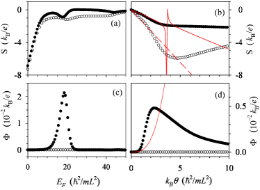
Figure 2: (Color online) Numerical results for the thermopower (a,b) and thermopower $B$-asymmetry (c,d) of a microjunction with an asymmetric scatterer [Fig. (1(b)] as a function of Fermi energy (a,c) and temperature (b,d). Full (open) symbols correspond to the presence (absence) of the voltage and thermal probe. Solid (dashed) lines in (b) are obtained using the Sommerfeld expansion to lowest order with (without) the probe. Note the strong deviation at moderately low temperatures. Solid line in (d) shows the $\Phi\propto\theta^{3}$ dependence of the $B$-asymmetry at low temperature. Parameters: magnetic length $\hbar c/eB=L^{2}$, temperature $k_{B}\theta=\hbar^{2}/mL^{2}$ (a,c) and Fermi energy $E_{F}=10\hbar^{2}/mL^{2}$ (b,d).

Numerical simulations. Clearly, for a chaotic cavity the thermopower magnetoasymmetry vanishes on average. Moreover, we expect the fluctuations to be exceedingly small since $\Phi$ depends, to leading order in $\theta$, on the second derivative of the transmission. Therefore, it is more natural to estimate the size of $\Phi$ in a different mesoscopic system—a microjunction as in Fig. 1(b). Thermopowers yielding 0.6 $\mu$V/K have been recently detected in a similar setup. mat11 The asymmetric scatterer deflects the electronic trajectories differently depending on the $B$ direction. Therefore, we expect an asymmetry in $S$ when $B$ is inverted.

Our prediction is confirmed by the numerical calculations of Fig. 2. We compute $T_{\alpha\beta}(E)$ using a grid discretization of the Schrödinger equation and, subsequently, the response coefficients from Eqs. (4)-(7) with Gauss-Legendre quadratures. suppl Upper panels show that adding the voltage and thermal probe reduces the thermopower absolute value as a function of both $E_{F}$ and $\theta$, in agreement with our previous results. In Fig. 2(b) we show that $S$ deviates from the lowest-order Sommerfeld expansion as temperature increases both with and without the probe. We emphasize that the thermopower is $B$-asymmetric only if the probe is present, as shown in Figs. 2(c,d). In Fig. 2d) we plot the asymmetry $\Phi$ as a function of temperature and show that $\Phi$ increases as $\theta^{3}$ at low temperature. The maximum value of $\Phi$ depends on the details of the scatterer and the system’s parameters. We find that $\Phi$ can reach values as high as $2$% for Fermi energies close to the activation of the second mode $E_{F}\simeq 19.7\hbar^{2}/mL^{2}$.

Conclusions. To summarize, we have investigated incoherent scattering effects on the thermoelectric transport of a mesoscopic conductor using a fictitious probe acting as an ideal potentiometer and thermometer. Our main findings are: (i) a general expression for the quantum fluctuations of the Seebeck coefficient upon elimination of the probe valid for both isothermal and adiabatic probes; (ii) a magnetic-field asymmetry of the thermopower, requiring both inelastic and dephasing processes, which becomes apparent only when higher-order terms are considered in a Sommerfeld expansion. Odd-in-$B$ thermopowers in Andreev interferometers have been experimentally observed cad09 and theoretically studied. jac10 We hope that our results will motivate the experimental detection of asymmetric thermopowers in normal systems.

Acknowledgments. We thank M. Büttiker and R. López for fruitful discussions. This work has been supported by the MICINN Grant No. FIS2008-00781.

SUPPLEMENTARY MATERIAL

.1 Details on Numerical Calculations

This section discusses in detail our numerical simulations for a few-mode mesoscopic conductor subject to incoherent scattering. We determine the set of multiterminal transmissions $T_{\alpha\beta}(E)$ using a grid discretization of the Schrödinger equation and solving the resulting linear equations, varying the boundary conditions for incidence from each of the leads. The leads are modelled as narrow waveguides with impenetrable hard walls, forming a T-junction geometry as sketched in Fig. 1(b) of the main paper. We also include an asymmetric triangular scatterer located at the center of the junction.

Magnetic field effects are modelled as follows. To avoid extended vector-potential fields $\vec{A}(\vec{r}\,)$ inside the leads, we consider the localized fields of Fig. 3, which might correspond to two coaxial coils of radii $R_{1}$ and $R_{2}$, perpendicular to the junction and carrying opposite currents. In this geometry $\vec{B}(\vec{r}\,)=B(r)\hat{u}_{z}$ and $\vec{A}(\vec{r}\,)=A(r)\hat{u}_{\phi}$, where $\hat{u}_{z}$ and $\hat{u}_{\phi}$ are the Cartesian and the azimuthal unit vectors, respectively, while $r$ is the distance from the junction center (Fig. 3). The field strengths read

$$\begin{array}[]{c|c|c}&B(r)&A(r)\\ \hline\cr r<R_{1}&B&\frac{B}{2}r\rule{0.0pt}{14.22636pt}\\ R_{1}<r<R_{2}&-B\frac{R_{1}^{2}}{R_{2}^{2}-R_{1}^{2}}&\frac{B}{2}\frac{R_{1}^{2}R_{2}^{2}}{R_{2}^{2}-R_{1}^{2}}\left(\frac{1}{r}-\frac{r}{R_{2}^{2}}\right)\rule{0.0pt}{14.22636pt}\\ r>R_{2}\rule{0.0pt}{14.22636pt}&0&0\end{array}\;,$$ (21)

Notice that, as required, not only $B(r)$, but also $A(r)$, vanishes in the leads when $r>R_{2}$. Therefore, our results arise purely from magnetic effects that occur within the junction only.

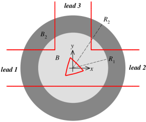
Figure 3: (Color online) Sketch of the magnetic field modelling, with the two regions of radii $R_{1}$ and $R_{2}$.

The central scatterer is modelled as a smooth two-dimensional barrier of height $V_{0}$ with a triangular shape in the plane. More specifically, the scatterer’s potential barrier in polar coordinates is given by

$$V(r,\theta)=\frac{V_{0}}{1+e^{(r-R_{T}(\theta))/\sigma_{T}}}\;,$$ (22)

where $R_{T}(\theta)$ is a piecewise function characterizing a triangle of side $L_{T}$ and oriented along a specific angle $\theta_{T}$, and $\sigma_{T}$ a small diffusivity.

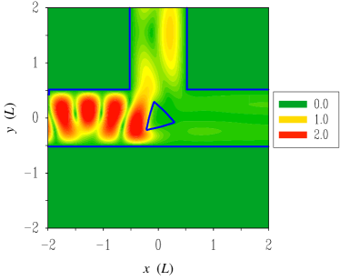
Figure 4: (Color online) Density distribution, $|\Psi(\vec{r}\,)|^{2}$, with $\Psi(\vec{r}\,)$ the solution of the Schrödinger equation for incidence from terminal 1 (left). The density is given in units of $L^{-2}$, where $L$ is the lateral extension of the leads. The position of the leads and the scatterer is indicated by solid lines. The incident energy is $E=30\hbar^{2}/mL^{2}$. Parameters of the magnetic field: $\hbar c/eB=L^{2}$, $R_{1}=L$, $R_{2}=1.5L$. Parameters of the repulsive scatterer: $V_{0}=200\hbar^{2}/mL^{2}$, $L_{T}=0.5L$, $\sigma_{T}=0.05L$, $\theta_{T}=15^{\rm o}$.

The numerical calculation of the kinetic terms including vector potential contributions is made using the Peierls substitution for lattice calculations. This is very convenient since it fulfills gauge invariance by construction. The practical implementation is as follows. We denote with $t_{ij}$ the finite-difference matrix associated with the kinetic energy on the grid. Thus, the operator acting on function $\Psi$ at grid point $i$ is given by the following sum over neighboring points $j$:

$$\left[\frac{(-i\hbar\nabla)^{2}}{2m}\Psi\right]_{i}=\sum_{j}{t}_{ij}\,\Psi_{j}\;.$$ (23)

The Peierls substitution for the vector potential terms amounts to including the following field-dependent phases in the sum

$$\left[\frac{1}{2m}\left(-i\hbar\nabla+\frac{e}{c}\vec{A}\right)^{2}\Psi\right]_{i}=\sum_{j}{t}_{ij}\,e^{{\frac{ie}{\hbar c}\frac{\vec{A}_{i}+\vec{A}_{j}}{2}\cdot(\vec{r}_{i}-\vec{r}_{j})}}\,\Psi_{j}\;.$$ (24)

As an example, Fig. 4 displays the probability density in the presence of scatterer and magnetic field in the case of incidence from the left (terminal 1).

Once the wave function for each incidence condition is known, it is an straightforward task to determine the quantum transmissions $T_{\alpha\beta}$ to be used in the evaluation of the linear transport coefficients, Eqs. (4)-(7) of the paper. These integrals are performed using a controlled numerical method, with the required precision ($10^{-5}$) achieved by successive partitioning of the integration domain in an increasing number of zones and computing each of them with a Gauss-Legendre method. In practice, the transmissions $T_{\alpha\beta}(E)$ for arbitrary energy $E$ are obtained by interpolating or extrapolating on a table of closely spaced precomputed values. Special care is taken for $E$ values close to the transverse mode energies to keep the discontinuities at these energies of the transmissions.

I Low temperature dependence

In this section, we show that at low temperature the thermopower asymmetry has a $\theta^{3}$ dependence. We present our analysis, both numerical and analytical, of this limit. We recall that the thermopower $B$-asymmetry $\Phi=S(B)-S(-B)$ reads,

$$\Phi=\frac{G_{33}(L_{13}K_{31}-L_{31}K_{13})+L_{33}(G_{31}K_{13}-G_{13}K_{31})+K_{33}(G_{13}L_{31}-G_{31}L_{13})}{\theta L_{33}(G_{11}L_{33}-G_{31}L_{13})+G_{33}(\theta L_{13}L_{31}+G_{11}K_{33})-G_{13}(G_{31}K_{33}+\theta L_{31}L_{33})}\,,$$ (25)

where the transport coefficients are given by

$$G_{\alpha\beta} =g_{V}(N_{\alpha}\delta_{\alpha\beta}-T_{\alpha\beta})\,,$$ (26)

$$L_{\alpha\beta} =g_{\theta}T_{\alpha\beta}^{\prime}\,,$$ (27)

$$K_{\alpha\beta} =-g_{\theta}(N_{\alpha}\delta_{\alpha\beta}-T_{\alpha\beta})/e\,,$$ (28)

to leading order in the Sommerfeld expansion. Higher orders are $\mathcal{O}(\theta)^{3}$. It follows from Eqs. (26) and (28) that $K_{\alpha\beta}=-(\pi^{2}k_{B}^{2}/3e^{2})\theta G_{\alpha\beta}$. Substituting this result in Eq. (20) one obtains $\Phi=0$. Therefore, nonzero magnetoasymmetries arise only if we carry out a Sommerfeld expansion for $K_{\alpha\beta}$ to higher order. We find,

$$K_{\alpha\beta}=-\frac{\pi^{2}k_{B}^{2}}{3e^{2}}\theta G_{\alpha\beta}+\frac{7\pi^{4}k_{B}^{4}}{15h}\theta^{3}T_{\alpha\beta}^{\prime\prime}+\mathcal{O}(\theta)^{5}\,.$$ (29)

Since $L_{\alpha\beta}$ is $\mathcal{O}(\theta)$, the numerator in the right-hand side of Eq. (25) is $\mathcal{O}(\theta)^{4}$, whereas the denominator is $\mathcal{O}(\theta)$. Then, the leading order of $\Phi$ is $\mathcal{O}(\theta)^{3}$.

Our numerical results are shown in Fig. 5, which displays a fit of $\Phi$ versus $\theta$ (dots) to a cubic-law behavior (line). The behavior predicted above is in agreement with the numerical data at low temperature. Obviously, higher-order contributions start to dominate as temperature increases. For the asymmetric microjunction, we estimate that the thermopower asymmetry deviates from the $\theta^{3}$ law at $k_{B}\theta\gtrsim\hbar^{2}/mL^{2}$.

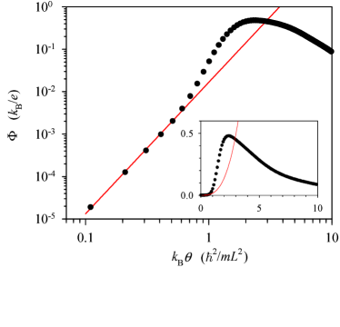
Figure 5: (Color online) Low temperature fit of the thermopower asymmetry, $\Phi\propto\theta^{3}$. Logarithmic scale is used in the main plot to highlight the low temperature region. For comparison, the inset shows the same data in linear scale. We use the same parameters as in Fig. 3(d) of the main paper: $E=10\hbar^{2}/mL^{2}$, $\hbar c/eB=L^{2}$, $R_{1}=L$, $R_{2}=1.5L$, $V_{0}=200\hbar^{2}/mL^{2}$, $L_{T}=0.5L$, $\sigma_{T}=0.05L$ and $\theta_{T}=15^{\rm o}$.

References

- (1) F. Giazotto, T.T. Heikkilä, A. Luukanen, A.M. Savin, and J.P. Pekola, Rev. Mod. Phys. 78, 217 (2006).
- (2) M. Terraneo, M. Peyrard, and G. Casati, Phys. Rev. Lett. 88, 094302 (2002).
- (3) L. Wang and B. Li, Phys. Rev. Lett. 99, 177208 (2007).
- (4) L.E. Bell, Science 321, 1457 (2008).
- (5) R. Sánchez and M. Büttiker, Phys. Rev. B 83, 085428 (2010).
- (6) P. Reddy, S-Y. Jang, R.A. Segalman, and A. Majumdar, Science 315, 1568 (2007).
- (7) M. Leijnse, M. R. Wegewijs, and K. Flensberg, Phys. Rev. B 82, 045412 (2010).
- (8) O. Entin-Wohlman, Y. Imry, and A. Aharony, Phys. Rev. B 82, 115314 (2010)
- (9) M. Büttiker, Phys. Rev. B 33, 3020 (1986); IBM J. Res. Dev. 32, 63 (1988).
- (10) H.U. Baranger and P.A. Mello, Phys. Rev. B 51, 4703 (1995).
- (11) P.W. Brouwer and C.W.J. Beenakker, Phys. Rev. B 55, 4695 (1997).
- (12) P.A. Jacquet, J. Stat. Phys. 134, 709 (2009).
- (13) P.N. Butcher, J. Phys.: Condens. Matter 2, 4869 (1990).
- (14) L.W. Molenkamp, Th. Gravier, H. van Houten, O.J.A. Buijk, M.A.A. Mabesoone, and C.T. Foxon, Phys. Rev. Lett. 68, 3765 (1992).
- (15) S.F. Godijn, S. Möller, H. Buhmann, L.W. Molenkamp, and S.A. van Langen, Phys. Rev. Lett. 82, 2927 (1999); A.S. Dzurak, C.G. Smith, C.H.W. Barnes, M. Pepper, L. Martín-Moreno, C.T. Liang, D.A. Ritchie, and G.A.C. Jones, Phys. Rev. B 55, 10197(R) (1997).
- (16) J. Matthews, D. Sánchez, M. Larsson, and H. Linke, arXiv:1107.3179 (preprint, 2011).
- (17) G. Benenti, K. Saito, and G. Casati, Phys. Rev. Lett. 106, 230602 (2011).
- (18) K. Saito, G. Benenti, G. Casati, and T. Prosen, Phys. Rev. B 84, 201306(R) (2011).
- (19) Y. Ming, Z.X. Wang, Z.J. Ding, and H.M. Li, New J. Phys. 12, 103041 (2010).
- (20) H.-L. Engquist and P.W. Anderson, Phys. Rev. B 24, 1151 (1981).
- (21) A. Caso, L. Arrachea, and G.S. Lozano, Phys. Rev. B 81, 041301(R) (2010).
- (22) A.G. Huibers, S.R. Patel, C.M. Marcus, P.W. Brouwer, C.I. Duruöz, and J.S. Harris, Jr., Phys. Rev. Lett. 81, 1917 (1998).
- (23) H.U. Baranger and P.A. Mello, Phys. Rev. Lett. 73, 142 (1994); R.A. Jalabert, J.-L. Pichard, and C.W.J. Beenakker, Europhys. Lett. 27, 255 (1994).
- (24) K. Schwab, E.A. Henriksen, J.M. Worlock, and M.L. Roukes, Nature 404, 974 (2000).
- (25) M.L. Polianski and P.W. Brouwer, J. Phys. A: Math. Gen. 36, 3215 (2003).
- (26) S.A. van Langen, P.G. Silvestrov, and C.W.J. Beenakker, Superlattices and Microstructures 23, 691 (1998).
- (27) D. Sánchez and M. Büttiker, Phys. Rev. Lett. 93, 106802 (2004); Int. J. Quant. Chem., 105, 906 (2005).
- (28) See supplementary material for details on the low temperature dependence of the thermopower asymmetry and on our numerical simulations.
- (29) N.W. Ashcroft and N.D. Mermin, Solid State Physics, Saunders College (1976), p. 761.
- (30) P. Cadden-Zimansky, J. Wei, and V. Chandrasekhar, Nature Physics 5, 393 (2009).
- (31) Ph. Jacquod and R.S. Whitney, Europhys. Lett. 91, 67009 (2010).