Taub-NUT Crystal

Harunobu Imazato^♯, Shun’ya Mizoguchi${}^{\sharp~{}\!\!\flat}$ and Masaya Yata^♯

^♯ Department of Particle and Nuclear Physics
The Graduate University for Advanced Studies
Tsukuba, Ibaraki 305-0801, Japan

^♭ Theory Center
High Energy Accelerator Research Organization (KEK)

Tsukuba, Ibaraki 305-0801, Japan

Abstract

We consider the Gibbons-Hawking metric for a three-dimensional periodic array of multi-Taub-NUT centers, containing not only centers with a positive NUT charge but also ones with a negative NUT charge. The latter are regarded as representing the asymptotic form of the Atiyah-Hitchin metric. The periodic arrays of Taub-NUT centers have close parallels with ionic crystals, where the Gibbons-Hawking potential plays the role of the Coulomb static potential of the ions, and are similarly classified according to their space groups. After a periodic identification and a ${\bf Z}_{2}$ projection, the array is transformed by T-duality to a system of NS5-branes with the SU(2) structure, and a further standard embedding yields, though singular, a half-BPS heterotic 5-brane background with warped compact transverse dimensions. A discussion is given of the possibility of probing the singular geometry by two-dimensional gauge theories.

July 2011

1 Introduction

Branes and singularities are essential ingredients in modern string theory. On one hand, branes are non-perturbative objects whose existence is required for consistency of various dualities. On the other hand, singularities are sources from which the effects of such objects emerge by allowing them to wrap around collapsing cycles. Branes and/or singularities are also required in order to realize inflation in string theory; under some mild assumptions, it was shown that smooth compactifications cannot allow an accelerating solution [1]. One way to circumvent this is to consider warped compactification with branes or singularities. There is a growing literature on attempts to realize a Randall-Sundrum-like framework [2] in string theory by using D-branes [3, 4, 5].

It has been known that, in order to achieve warped compactification in supergravity, some of the constituent branes need to have negative tension [4]. (This fact was shown in type IIB theory but can be generalized to other string theories.) In type II theories, an orientifold has this property. In heterotic string theory, however, one cannot define orientifolds as one does in type II theories, since, while one needs to gauge world-sheet parity to define orientifolds, heterotic theory is left-right asymmetric and hence does not possess such a symmetry to be gauged. Although even in the absence of the worldsheet definition one can define orientifolds by simply assigning ${\bf Z}_{2}$ actions on various fields [6], it is unclear what kind of geometry is produced there. The back-reaction problem of orientifolds was considered in [7].

In this paper, we propose a novel, interesting set up for warped compactification of heterotic (as well as type II) string theory to six dimensions, based on a simple idea: We consider the Gibbons-Hawking metric [8] for a three-dimensional periodic array of multi-Taub-NUT centers consisting of not only centers with a positive NUT charge but also ones having a negative NUT charge. This negative-charge metric is regarded as representing the asymptotic form of the Atiyah-Hitchin metric; as is well known, the Atiyah-Hitchin metric [9] is a smooth self-dual metric on a Euclidean four-manifold, and it looks like a negative-charge Taub-NUT for an observer who is far enough from the bolt locus. Such a periodic array of infinite Taub-NUT centers was already discussed in [10, 11]. The idea of introducing an Atiyah-Hitchin space in the Gibbons-Hawking metric was used in [12] to understand how an $SO(2n)$ gauge symmetry enhancement occurs due to D-branes. By T-duality, the periodic array of Taub-NUT centers is converted to a periodic array of NS5-branes. An ordinary (positive-charge) Taub-NUT is T-dualized to a (smeared) NS5-brane, and the negative-charge Taub-NUT is mapped to a (smeared) negative-tension brane. The resulting T-dual system has the $SU(2)$ structure (hyper-Kähler with torsion), and preserves one half the supersymmetries. We then embed the generalized spin connection into gauge connection to obtain a 5-brane system with a compact four-dimensional transverse space in heterotic string theory.

As is known, although the negative-NUT approximation of the Atiyah-Hitchin metric is good at large distances compared to the NUT-charge scale, near the center the approximate metric becomes singular on a two-dimensional sphere (in the three-dimensional space where the periodic array is defined) of radius equal to the NUT charge. Therefore, on the T-dual side, there are two kinds of regions where the supergravity analysis is not reliable: One is the region near a smeared NS5-brane, the familiar one where the geometry is an infinite throat and the dilaton blows up as one approaches the core. The other is the region near the brane dual to the nagative-charge Taub-NUT center, in which, unlike the above, both the metric and the dilaton go to zero as one approaches the singularity surface, and inside it the metric becomes negative and the space ceases to be Riemannian. The former is a common difficulty, while the latter singularity is the one inherited from the “one-loop approximation” of the Atiyah-Hitchin metric without taking into account the instanton effects. Nevertheless, despite the existence of these regions, we would like to emphasize that our construction is interesting in the following points:

First, it clarifies the origin of orientifold-like objects in heterotic string theory; such objects are necessary to be included to neutralize the total NUT charge before T-duality. Indeed, their T-duals are very similar to orientifolds; the ${\bf Z}_{2}$ projection naturally arises from the bolt of the Atiyah-Hitchin space, and the ADM energy per unit area is negative. The second point we wish to make is that our 5-brane system is not just being a singular geometry, but suggests how the nonperturbative effects (by vortices in the corresponding gauge theory) correct the geometry. Although incomplete, we will consider in a later section the relevant $(4,4)$ sigma models whose leading-order moduli spaces are singular 5-brane geometries above but vortex corrections may change them. The problem amounts to finding a possible deformation of hyper-Kähler geometry with torsion, and the sigma model [13] analysis may provide a systematic way.

The infinite periodic array of Taub-NUT centers that we describe is similar to three-​ dimensional ionic crystals, such as sodium chloride (NaCl), cesium chloride (CsCl), etc., where the Atiyah-Hitchin’s and Taub-NUT’s correspond to minus and plus ions in the crystal, and the Gibbons-Hawking potential plays the role of the Coulomb static potential of the ions. Generically, the Gibbons-Hawking potential for such a three-dimensional periodic array does not converge, even if the total NUT charge of a unit cell is neutralized. As we will see shortly, the condition for convergence is that the positive- and negative-charge centers are arranged in a unit cell in such a way that the leading difference operator of the multipole expansion of the potential becomes proportional to the discrete Laplace operator. This condition constrains the locations of the Taub-NUT centers relative to the Atiyah-Hitchin centers, that is, the ones with negative NUT charge. Another constraint for the positions of the Taub-NUT centers is that they must be inversion symmetric with respect to every Atiyah-Hitchin bolt locus so that they are consistent with the ${\bf Z}_{2}$ identification around the bolt. Thus, while a real crystal is mathematically described as a three-dimensional torus, the “Taub-NUT crystal” is a certain orbifold.

The plan of this paper is as follows: In section 2 we review the basic facts about the Atiyah-Hitchin metric. In section 3 we give a definition of our set up by introducing a three-dimensional periodic array of Taub-NUT centers, and examine the convergence condition for the Gibbons-Hawking potential. A relation to the $K_{3}$ orientifold is discussed, and the classification of the crystal structure is also described there. In section 4 we take T-duality of the Taub-NUT crystal to obtain a 5-brane system with compact transverse dimensions, and then we embed it into heterotic string theory. At the end of this section we briefly discuss possible corrections to the singularity from the point of view of the nonlinear sigma model approach. Section 5 is devoted to a summary. An appendix contains some details of the Darboux-Halphen system, where comparisons are also made between the solutions in the literature.

2 The Atiyah-Hitchin metric

Let us first recall some basic properties of the Atiyah-Hitchin metric. The Atiyah-Hitchin metric is a smooth metric on a Euclidean four-manifold with a(n) (anti-)self-dual Riemann curvature without triholomorphic $U(1)$ isometry. It is written as a special Bianichi IX metric of the form

$$ds^{2}=a^{2}b^{2}c^{2}dt^{2}+a^{2}\sigma_{1}^{2}+b^{2}\sigma_{2}^{2}+c^{2}\sigma_{3}^{2},$$ (2.1)

where $a$, $b$ and $c$ are functions of $t$ only. $\sigma_{i}$’s $(i=1,2,3)$ are the Maurer-Cartan 1-forms of $SU(2)$ given by

$$\sigma_{1} = -\sin\psi d\theta+\sin\theta\cos\psi d\phi,$$

$$\sigma_{2} = \cos\psi d\theta+\sin\theta\sin\psi d\phi,$$ (2.2)

$$\sigma_{3} = d\psi+\cos\theta d\phi.$$

In terms of a new set of functions

$$w_{1}=bc,~{}w_{2}=ca,~{}w_{3}=ab,$$ (2.3)

a (sufficient) condition for a(n) (anti-)self curvature is that they fulfill the Darboux-Halphen system

$$\dot{w}_{1}+\dot{w}_{2}=2w_{1}w_{2},$$

$$\dot{w}_{2}+\dot{w}_{3}=2w_{2}w_{3},$$ (2.4)

$$\dot{w}_{3}+\dot{w}_{1}=2w_{3}w_{1}.$$

For our purpose, a convenient representation of solutions is the one in terms of elliptic theta functions [14, 15]

$$w_{j}(t) = 2\frac{d}{dt}\log\vartheta_{j+1}(0,i\alpha t)~{}~{}~{}(j=1,2,3),$$ (2.5)

where $\alpha>0$ is an arbitrary constant parameter. We will see that this $\alpha$ is related to the NUT charge of the asymptotic Taub-NUT metric. The obtained self-dual metric is thus

$$ds^{2} = 2\left(\prod_{j=3,4,2}\frac{d}{dt}\log\vartheta_{j}(0,i\alpha t)\right)\left(4dt^{2}+\frac{\sigma_{1}^{2}}{(\frac{d}{dt}\log\vartheta_{2}(0,i\alpha t))^{2}}\right.$$ (2.6)

$$~{}~{}~{}~{}~{}~{}~{}~{}~{}~{}~{}~{}~{}~{}~{}~{}~{}~{}~{}~{}~{}~{}~{}~{}~{}~{}~{}~{}~{}~{}~{}~{}~{}~{}~{}~{}~{}\left.+\frac{\sigma_{2}^{2}}{(\frac{d}{dt}\log\vartheta_{3}(0,i\alpha t))^{2}}+\frac{\sigma_{3}^{2}}{(\frac{d}{dt}\log\vartheta_{4}(0,i\alpha t))^{2}}\right).$$

In this representation of the solutions, Atiyah-Hitchin’s original solution corresponds to $\alpha=\pi$, whereas Gibbons-Manton’s solution to $\alpha=2\pi$ (with replacing the radial coordinate $t$ by $-\eta$. See Appendix for more detail.).

It is well known [16] (also see [17] for a review) that, on one hand, the Atiyah-Hitchin metric develops a removable “bolt” singularity at the origin (in a certain coordinate system), and on the other hand, it rapidly approaches to a Taub-NUT metric with negative NUT charge asymptotically. Although these are well-known facts, we include a brief derivation of them because they are essential in constructing a crystal structure in the space of Taub-NUT centers. These behaviors can be conveniently confirmed in our representation of solutions in terms of theta functions [15].

(i) The behavior near $t=\infty$: The bolt

The elliptic theta functions are readily given as an infinite series as

$$\vartheta_{3}(0,\tau) = \sum_{n\in{\bf Z}}q^{\frac{1}{2}n^{2}},$$

$$\vartheta_{4}(0,\tau) = \sum_{n\in{\bf Z}}(-1)^{n}q^{\frac{1}{2}n^{2}},$$ (2.7)

$$\vartheta_{2}(0,\tau) = \sum_{n\in{\bf Z}}q^{\frac{1}{2}(n-\frac{1}{2})^{2}},$$

with $q=e^{2\pi i\tau}$. Putting $\tau=i\alpha t$, the $t\rightarrow\infty$ limit of (2.5) can be obtained by taking the leading terms of the expansions:

$$w_{2}(t) \stackrel{{\scriptstyle t\rightarrow\infty}}{{\sim}} 2\frac{d}{dt}\log(1+2e^{-\pi\alpha t}+\cdots)$$

$$= -4\pi\alpha~{}e^{-\pi\alpha t}+\cdots,$$

$$w_{3}(t) \stackrel{{\scriptstyle t\rightarrow\infty}}{{\sim}} 2\frac{d}{dt}\log(1-2e^{-\pi\alpha t}+\cdots)$$ (2.8)

$$= +4\pi\alpha~{}e^{-\pi\alpha t}+\cdots,$$

$$w_{1}(t) \stackrel{{\scriptstyle t\rightarrow\infty}}{{\sim}} 2\frac{d}{dt}\log(2e^{-\frac{\pi}{4}\alpha t}+\cdots)$$

$$= -\frac{\pi}{2}\alpha+\cdots.$$

Therefore, $a$,$b$ and $c$ are

$$a^{2} = \frac{w_{2}w_{3}}{w_{1}}~{}\stackrel{{\scriptstyle t\rightarrow\infty}}{{\sim}}~{}32\pi\alpha e^{-2\pi\alpha t}+\cdots,$$

$$b^{2} = \frac{w_{3}w_{1}}{w_{2}}~{}\stackrel{{\scriptstyle t\rightarrow\infty}}{{\sim}}~{}\frac{\pi}{2}\alpha+\cdots,$$

$$c^{2} = \frac{w_{1}w_{2}}{w_{3}}~{}\stackrel{{\scriptstyle t\rightarrow\infty}}{{\sim}}~{}\frac{\pi}{2}\alpha+\cdots.$$

The metric takes the form

$$ds^{2} \stackrel{{\scriptstyle t\rightarrow\infty}}{{\sim}} 8\pi\alpha(\pi^{2}\alpha^{2}e^{-2\pi\alpha t}dt^{2}+4e^{-2\pi\alpha t}\sigma_{1}^{2})+\frac{\pi}{2}\alpha(\sigma_{2}^{2}+\sigma_{3}^{2}).$$ (2.9)

This is a bolt; by a change of coordinates $u\equiv e^{-\pi\alpha t}$, the metric becomes

$$ds^{2} = 8\pi\alpha(du^{2}+4u^{2}\sigma_{1}^{2})+\frac{\pi}{2}\alpha(\sigma_{2}^{2}+\sigma_{3}^{2}).$$ (2.10)

Defining the new angle coordinates [16] such that

$$\sigma_{1} = d\tilde{\psi}+\cos\tilde{\theta}d\tilde{\phi},$$

$$\sigma_{2} = -\sin\tilde{\psi}d\tilde{\theta}+\sin\theta\cos\tilde{\psi}d\tilde{\phi},$$ (2.11)

$$\sigma_{3} = \cos\tilde{\psi}d\tilde{\theta}+\sin\theta\sin\tilde{\psi}d\tilde{\phi},$$

we see that this metric is regular at $u=0$ ($t=\infty$) if $0\leq\tilde{\psi}\leq\pi$, that is, the points at the angles $\tilde{\psi}$ and $\tilde{\psi}+\pi$ must be identified. This ${\bf Z}_{2}$ transformation acts on the original angle variables as

$$\theta \mapsto \pi-\theta,$$

$$\phi \mapsto \phi+\pi,$$ (2.12)

$$\psi \mapsto -\psi.$$

This means that the space around the Atiyah-Hitchin bolt locus gets ${\bf Z}_{2}$ orbifolded. Later this fact places a significant constraint on our construction of the Taub-NUT crystal.

(ii) The behavior near $t=0$: The negative Taub-NUT

To investigate the asympotics near $t=0$, one needs to consider the modular $S$ transformations of the theta functions [15]:

$$\vartheta_{3}\left(0,-\frac{1}{i\alpha t}\right) = \sqrt{\alpha t}~{}\vartheta_{3}(0,i\alpha t),$$

$$\vartheta_{4}\left(0,-\frac{1}{i\alpha t}\right) = \sqrt{\alpha t}~{}\vartheta_{2}(0,i\alpha t),$$ (2.13)

$$\vartheta_{2}\left(0,-\frac{1}{i\alpha t}\right) = \sqrt{\alpha t}~{}\vartheta_{4}(0,i\alpha t).$$

Using (2.13), we can similarly obtain

$$w_{2}(t) = 2\frac{d}{dt}\log\left(\frac{1}{\sqrt{\alpha t}}~{}\vartheta_{3}(0,\frac{i}{\alpha t})\right)$$

$$\stackrel{{\scriptstyle t\rightarrow 0}}{{\sim}} -\frac{1}{t}+\cdots,$$

$$w_{3}(t) = 2\frac{d}{dt}\log\left(\frac{1}{\sqrt{\alpha t}}~{}\vartheta_{2}(0,\frac{i}{\alpha t})\right)$$ (2.14)

$$\stackrel{{\scriptstyle t\rightarrow 0}}{{\sim}} \frac{\pi}{2\alpha t^{2}}-\frac{1}{t}+\cdots,$$

$$w_{1}(t) = 2\frac{d}{dt}\log\left(\frac{1}{\sqrt{\alpha t}}~{}\vartheta_{4}(0,\frac{i}{\alpha t})\right)$$

$$\stackrel{{\scriptstyle t\rightarrow 0}}{{\sim}} -\frac{1}{t}+\cdots,$$

where the ellipses stand for the terms containing a power of $e^{-\frac{\pi}{\alpha t}}$. If those contributions are discarded, the $a$, $b$ and $c$ functions reduce to

$$a^{2} \stackrel{{\scriptstyle t\rightarrow 0}}{{\sim}} \frac{\pi-2\alpha t}{2\alpha t^{2}},$$

$$b^{2} \stackrel{{\scriptstyle t\rightarrow 0}}{{\sim}} \frac{\pi-2\alpha t}{2\alpha t^{2}},$$ (2.15)

$$c^{2} \stackrel{{\scriptstyle t\rightarrow 0}}{{\sim}} \frac{2\alpha}{\pi-2\alpha t}.$$

The metric approaches to

$$ds^{2} \stackrel{{\scriptstyle t\rightarrow 0}}{{\sim}} \frac{\pi-2\alpha t}{2\alpha t^{4}}dt^{2}+\frac{2\alpha}{\pi-2\alpha t}\sigma_{3}^{2}+\frac{\pi-2\alpha t}{2\alpha t^{2}}(\sigma_{1}^{2}+\sigma_{2}^{2})$$ (2.16)

$$= \left(1-\frac{\sqrt{\frac{2\alpha}{\pi}}}{r}\right)\left(dr^{2}+r^{2}(\sigma_{1}^{2}+\sigma_{2}^{2})\right)+\frac{2\alpha}{\pi}\left(1-\frac{\sqrt{\frac{2\alpha}{\pi}}}{r}\right)^{-1}\sigma_{3}^{2},$$

where we have changed variables from $t$ to $r=(\sqrt{\frac{2\alpha}{\pi}}t)^{-1}$ in the second line. (2.16) is a Taub-NUT metric with negative NUT charge $-\sqrt{\frac{2\alpha}{\pi}}$ [16].

As was noted in [16], this approximate metric (2.16) is singular at $r=\sqrt{\frac{2\alpha}{\pi}}$; this is an artifact of the absence of the exponential terms ignored in the theta functions. On the other hand, the smooth, self-dual metric (2.6) rapidly approaches to the approximate metric (2.16) as $r\rightarrow\infty$, and for an observer outside a radius of the NUT charge scale, it looks as if there is a Taub-NUT with negative NUT charge, which has an $U(1)$ isometry. Later we take T-duality of this approximate metric along this isometry.

3 Taub-NUT crystal

3.1 Infinite periodic array of Taub-NUT centers

In the previous section we have seen that the Atiyah-Hitchin space can be approximately identified as a negative-charge Taub-NUT space at large distances compared to the NUT charge scale. Motivated by this observation, in this section we consider the Gibbons-Hawking metric for an infinite periodic array of Taub-NUT centers, where some of them in the unit cell have negative NUT charge. The idea is that, by periodically identifying such an infinite array, one obtains an $S^{1}$ fibered three-dimensional torus with (anti-)self-dual metric, and by T-duality it is mapped to an NS5-brane system with compact transverse dimensions, where some of the 5-branes have negative tension.

The Gibbons-Hawking metric [8]

$$ds_{GH}^{2} = V(\vec{x})d\vec{x}^{2}+V^{-1}(\vec{x})(dx_{9}+\vec{\omega}\cdot d\vec{x})^{2},$$ (3.1)

$$V(\vec{x}) = \varepsilon+\sum_{k=1}^{N}\frac{2m}{|\vec{x}-\vec{x}_{k}|},$$ (3.2)

$$\vec{\nabla}V = \vec{\nabla}\times\vec{\omega},$$ (3.3)

is an anti-self-dual metric in a four-dimensional Euclidean space with coordinates $(\vec{x},x_{9})$, $\vec{x}=(x,y,z)$. We have used the subscript $9$, anticipating that this metric will be embedded in string theory. $\varepsilon$ and $m$ are constants. If $\varepsilon\neq 0$, the metric describes a multi-center Taub-NUT space, while if $\varepsilon=0$, the metric is the one for the $A_{N-1}$ singularity [18]. If $\varepsilon\neq 0$, it can be arranged to $1$ by making a suitable change of coordinates, so we can set $\varepsilon=1$ for the Taub-NUT case without loss of generality. Then if $N=1$ and the center $\vec{x}_{1}$ is taken at the origin $\vec{0}$, the potential $V$ takes the form

$$V(\vec{x})=1+\frac{2m}{r}~{}~{}~{}(r=\sqrt{x^{2}+y^{2}+z^{2}}).$$ (3.4)

Choosing the gauge $\omega_{z}=0$, $\vec{\omega}$ can be determined (for the anti-self-dual case) as

$$\vec{\omega} = \left(-\frac{2myz}{(x^{2}+y^{2})r},\frac{2mxz}{(x^{2}+y^{2})r},0\right).$$ (3.5)

Then the metric (3.1) reads

$$ds_{GH}^{2}(N=1) = \left(1+\frac{2m}{r}\right)d\vec{x}^{2}+\frac{1}{1+\frac{2m}{r}}\left(dx_{9}+2m\frac{z}{r}d\left(\tan^{-1}\frac{y}{x}\right)\right)^{2}.$$ (3.6)

By a change of coordinates

$$x = r\sin\theta\cos\phi,$$

$$y = r\sin\theta\sin\phi,$$

$$z = r\cos\theta,$$

$$x_{9} = 2m\psi,$$ (3.7)

(3.6) is reduced to a Taub-NUT metric with NUT charge $2m$:

$$ds_{GH}^{2}(N=1) = \left(1+\frac{2m}{r}\right)(dr^{2}+r^{2}(\sigma_{1}^{2}+\sigma_{2}^{2}))+4m^{2}\left(1+\frac{2m}{r}\right)^{-1}\sigma_{3}^{2}.$$ (3.8)

Going back to the general $N$ case, we impose the following conditions on the configuration of centers:

1. For every location of a negative NUT charge $\vec{x}_{0}$, the configuration is invariant under the ${\bf Z}_{2}$ transformation :

$$\vec{x}-\vec{x}_{0} \mapsto -(\vec{x}-\vec{x}_{0})$$ (3.9)

(called inversion in the terminology of crystallography).

2. The superposition of infinitely many Gibbons-Hawking potentials converges.

The first condition is imposed in order for each negative-charge center to consistently represent the asymptotic region of the Atiyah-Hitchin geometry. To recover correctly the original Atiyah-Hitchin metric in the non-compact limit where the negative-charge NUT is isolated from the positive ones, the image of the inversion (3.9) needs to be identified, as we saw in the previous section.

The second condition is obvious; a Gibbons-Hawking potential from a single nut falls like $1/|\vec{x}|$, and due to the condition 1 the leading asymptotic behavior of the superposition is $1/|\vec{x}|^{3}$ generically, and therefore the summation over a three-dimensional lattice diverges logarithmically. The superposition of the potentials converges if and only if the positive- and negative-charge centers are arranged in a unit cell in such a way that the leading order term of the multipole expansion vanishes. We will present a precise description of the condition in the next section. Note that the situation is completely analogous to the Coulomb static potential in a crystal system, and any actual ionic crystals consisting of two oppositely charged ions will satisfy this condition.

In addition, we also assume for simplicity that

3. There are no orbifold fixed points besides the locations of negative charges.

Then a little thought shows that the Gibbons-Hawking potential $V(x)$ takes the form

$$V(\vec{x}) = 1+\sum_{\rule{0.0pt}{4.52083pt}n_{1},n_{2},n_{3}\in{\bf{Z}}}\sum_{\epsilon_{1},\epsilon_{2},\epsilon_{3}\in\{0,\frac{1}{2}\}}V^{(\epsilon_{1},\epsilon_{2},\epsilon_{3})}({\textstyle\vec{x}-\sum_{j=1}^{3}n_{j}\vec{y}_{j}}),$$ (3.10)

$$V^{(\epsilon_{1},\epsilon_{2},\epsilon_{3})}(\vec{x}) = \frac{-4mN^{(\epsilon_{1},\epsilon_{2},\epsilon_{3})}}{\left|\vec{x}-\sum_{j=1}^{3}\epsilon_{j}\vec{y}_{j}\right|}+\sum_{k=1}^{N^{(\epsilon_{1},\epsilon_{2},\epsilon_{3})}}\left(\frac{2m}{\left|\vec{x}-\vec{x}_{k}^{~{}(\epsilon_{1},\epsilon_{2},\epsilon_{3})}-\sum_{j=1}^{3}\epsilon_{j}\vec{y}_{j}\right|}\right.$$ (3.11)

$$~{}~{}~{}~{}~{}~{}~{}~{}~{}~{}~{}~{}~{}~{}~{}~{}~{}~{}~{}~{}~{}~{}~{}~{}~{}~{}~{}~{}~{}~{}~{}~{}~{}~{}~{}\left.+\frac{2m}{\left|\vec{x}+\vec{x}_{k}^{~{}(\epsilon_{1},\epsilon_{2},\epsilon_{3})}-\sum_{j=1}^{3}\epsilon_{j}\vec{y}_{j}\right|}\right),$$

where ${\vec{y}}_{j}\in{\bf R}^{3}$ $(j=1,2,3)$ are the period vectors of the array.

The unit cell of the periodic array is a parallelepiped specified by ${\vec{y}}_{j}$ $(j=1,2,3)$, which contains eight ($\epsilon_{j}\in\{0,\frac{1}{2}\}$ for $j=1,2,3$) subunits (Figure).

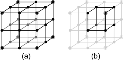
Figure 1: (a) A Unit cell and (b) a subunit of the Taub-NUT crystal. The dots are the positions of negative-charge centers, of which the circled ones are identified periodically. Positive-charge centers, which are not depicted in these figures, must be placed symmetrically with respect to the inversion through any dot.

Each subunit specified by $(\epsilon_{1},\epsilon_{2},\epsilon_{3})$ of the array consists of one negative-charge center with NUT charge $-4mN^{(\epsilon_{1},\epsilon_{2},\epsilon_{3})}$ and $N^{(\epsilon_{1},\epsilon_{2},\epsilon_{3})}$ pairs of positive-charge centers with a common NUT charge $2m$, which are placed symmetrically with respect to the position of the negative-charge center. The relative positions of the $k$th pair ($k=1,\ldots,,N^{(\epsilon_{1},\epsilon_{2},\epsilon_{3})}$) are $\pm\vec{x}_{k}^{~{}(\epsilon_{1},\epsilon_{2},\epsilon_{3})}$. The potential $V^{(\epsilon_{1},\epsilon_{2},\epsilon_{3})}(\vec{x})$ arises from these centers belonging to the subunit $(\epsilon_{1},\epsilon_{2},\epsilon_{3})$.

We now periodically identify points as

$$(\vec{x},x_{9}) \sim \left(\vec{x}+\sum_{j=1}^{3}m_{j}\vec{y}_{j},x_{9}\right)~{}~{}~{}(m_{j}\in{\bf Z})$$ (3.12)

and also take an orbifold

$$(\vec{x},x_{9}) \sim \left(-\vec{x}+2\sum_{j=1}^{3}(n_{j}+\epsilon_{j})\vec{y}_{j},-x_{9}\right)~{}~{}~{}(n_{j}\in{\bf Z},~{}~{}\epsilon_{j}\in{\{0,{\textstyle\frac{1}{2}}\}}),$$ (3.13)

as we mentioned above. The metric (3.1) with (3.10),(3.11) and (3.3) is invariant under the operations (3.12) and (3.13) and the identifications can consistently be done.

Note that if there were only a single negative-charge center, (3.12) would identify points in spaces with opposite orientations and the quotient would become non-orientable. Also, there would appear orbifold fixed points besides their own locations. This is why we have introduced eight negative-charge centers in the unit cell.

3.2 Convergence condition

The metric (3.1) with (3.10),(3.11) and (3.3) is an infinite, periodic generalization of the Gibbons-Hawking metric. In this section we consider in what circumstances the potential $V$ converges. If the positive and negative centers are in generic positions, the potential (3.11) falls like $1/|\vec{x}|^{3}$ since it can be written as a sum of second order differences, and therefore the summation over a three-dimensional lattice diverges logarithmically. However, the exception to this is where the leading order term of the multipole expansion of

$$\sum_{\epsilon_{1},\epsilon_{2},\epsilon_{3}\in\{0,\frac{1}{2}\}}V^{(\epsilon_{1},\epsilon_{2},\epsilon_{3})}(\vec{x})$$ (3.14)

vanishes, that is, the positive- and negative-charge centers are arranged in a unit cell in such a way that the leading difference operator of the multipole expansion is proportional to the discrete Laplace operator.

The simplest example of a convergent potential is the case where the lattice is a cubic lattice

$$\vec{y}_{j}=2a\vec{n}_{j}~{}~{}~{}(j=1,2,3),$$ (3.15)

$$\vec{n}_{1}\equiv(1,0,0),~{}\vec{n}_{2}\equiv(0,1,0),~{}\vec{n}_{3}\equiv(0,0,1),$$ (3.16)

and all $V^{(\epsilon_{1},\epsilon_{2},\epsilon_{3})}(\vec{x})$’s are obtained as translations of an identical potential:

$$V^{(\epsilon_{1},\epsilon_{2},\epsilon_{3})}(\vec{x}) = V_{ReO_{3}}(\vec{x}-{\textstyle\sum_{j=1}^{3}\epsilon_{j}\vec{y}_{j}},\delta),$$ (3.17)

$$V_{ReO_{3}}(\vec{x},\delta) \equiv 2m\left(-\frac{6}{\left|\vec{x}\right|}+\sum_{j=1}^{3}\left(\frac{1}{|\vec{x}-\delta a\vec{n}_{j}|}+\frac{1}{|\vec{x}+\delta a\vec{n}_{j}|}\right)\right),$$ (3.18)

where $a$ is half the period of the array and $0<\delta\leq 1$ is a parameter (Figure 2 (a-1), (a-2)).

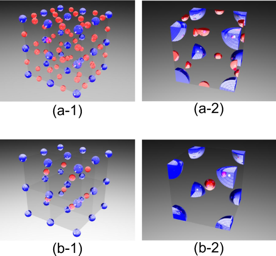
Figure 2: Examples of convergent configurations. The unit cells of (a-1) the $ReO_{3}$-type and (b-1) the $CsCl$-type crystals are depicted, and (a-2), (b-2) are their sub-units, respectively. The blue spheres show the positions of the negative-charge (“Atiyah-Hitchin”) centers, whereas the red ones are the positive-charge (“Taub-NUT”) centers.

Indeed, we can rewrite (3.18) as

$$2m\left(-\frac{6}{\left|\vec{x}\right|}+\sum_{j=1}^{3}\left(\frac{1}{|\vec{x}-\delta a\vec{n}_{j}|}+\frac{1}{|\vec{x}+\delta a\vec{n}_{j}|}\right)\right)$$ (3.19)

$$= 2m\sum_{j=1}^{3}\left(\left(\frac{1}{|\vec{x}+\delta a\vec{n}_{j}|}-\frac{1}{\left|\vec{x}\right|}\right)-\left(\frac{1}{\left|\vec{x}\right|}-\frac{1}{|\vec{x}-\delta a\vec{n}_{j}|}\right)\right)$$

$$= 2m\delta^{2}a^{2}\sum_{j=1}^{3}(\vec{n}_{j}\cdot\vec{\nabla})^{2}\frac{1}{|\vec{x}|}+O(a^{4})$$

$$= 2m\delta^{2}a^{2}\Delta\frac{1}{|\vec{x}|}+O(a^{4}),$$

where $\Delta$ is the flat space Laplacian. The first term vanishes, and on dimensional grounds the rest falls like $|\vec{x}|^{-5}$ at least. Therefore the summation over the lattice converges.

Another simple example of a convergent potential is the case in which the lattice is again cubic and a subunit has four (pairs of) Taub-NUT’s per single Atiyah-Hitchin (Figure 2 (b-1), (b-2)):

$$V^{(\epsilon_{1},\epsilon_{2},\epsilon_{3})}(\vec{x}) = V_{CsCl}(\vec{x}-{\textstyle\sum_{j=1}^{3}\epsilon_{j}\vec{y}_{j}},\delta),$$ (3.20)

$$V_{CsCl}(\vec{x},\delta) \equiv 2m\left(-\frac{8}{\left|\vec{x}\right|}+\sum_{\xi_{1},\xi_{2},\xi_{3}=\pm 1}\frac{1}{\left|\vec{x}-\delta a\sum_{j=1}^{3}\xi_{j}\vec{n}_{j}\right|}\right).$$ (3.21)

More generally, if one requires that for each subunit $(\epsilon_{1},\epsilon_{2},\epsilon_{3})$ the leading-order term of $V^{(\epsilon_{1},\epsilon_{2},\epsilon_{3})}(\vec{x})$ in the large-$|\vec{x}|$ expansion vanishes, the condition for the relative positions of the Taub-NUT centers is that the $3\times N^{(\epsilon_{1},\epsilon_{2},\epsilon_{3})}$-matrix

$$X^{(\epsilon_{1},\epsilon_{2},\epsilon_{3})} \equiv \left(\vec{x}_{1}^{(\epsilon_{1},\epsilon_{2},\epsilon_{3})},\vec{x}_{2}^{(\epsilon_{1},\epsilon_{2},\epsilon_{3})},\ldots,\vec{x}_{N^{(\epsilon_{1},\epsilon_{2},\epsilon_{3})}}^{(\epsilon_{1},\epsilon_{2},\epsilon_{3})}\right)$$ (3.22)

should satisfy

$$X^{(\epsilon_{1},\epsilon_{2},\epsilon_{3})}{X^{(\epsilon_{1},\epsilon_{2},\epsilon_{3})}}^{T} = kI_{3}$$ (3.23)

for some constant $k$, where $I_{3}$ is the $3\times 3$ identity matrix. It is easy to see that the two examples above fulfill this condition.

Note that (3.23) is a sufficient condition for $V(\vec{x})$ to converge; it is enough if the sum (3.14) over the unit has the asymptotic fall-off is not slower than $|\vec{x}|^{-3}$, and each $V^{(\epsilon_{1},\epsilon_{2},\epsilon_{3})}(\vec{x})$ need not subunit-wise. Of course, in such a general case the crystal has less discrete symmetries, however.

3.3 Taub-NUT crystal as an approximation of $K_{3}$

The negative-charge metric (2.16) is singular, but adding exponential correction terms the singularity disappears and the metric becomes completely smooth to be the Atiyah-Hitchin metric. These exponential corrections are regarded as coming from certain instantons [19, 20, 15]. In the language of the corresponding gauge theory, this is a strong-coupling effect of the non-abelian ($=SU(2)$) gauge theory at low energies, where the location of the singularity surface corresponds to $\Lambda_{QCD}$. It is reasonable to expect that there will also be such corrections even after the three-dimensional lattice is compactified to be a torus. If this is true, and if these corrections can smooth out the singularity as they do in the non-compact case, then the resulting space must be a $K_{3}$ surface, as it is the only nontrivial smooth compact hyper-Kähler four-manifold. The compactified periodic array can then be regarded as an approximation of a $K_{3}$ surface (which is only valid except near the locations of the negative-charge centers). However, this can only happen if

$$\sum_{\epsilon_{1},\epsilon_{2},\epsilon_{3}\in\{0,\frac{1}{2}\}}N^{(\epsilon_{1},\epsilon_{2},\epsilon_{3})} = 16$$ (3.24)

in a unit cell since the Euler number of $K_{3}$ is 24. This means that (apparently, including their ${\bf Z}_{2}$ images) there are 32 positive-charge Taub-NUT centers in a unit cell before the ${\bf Z}_{2}$ identification. Note that although the number of negative-charge centers is apparently eight, it must be halved when counting the number of bolts due to the ${\bf Z}_{2}$ identification. (This is the same as the Euler-number counting of the $K_{3}$ orbifold [21], where the number of excised points is not equal to the number of the fixed points itself, but it must be divided by the order of the orbifold.) Therefore, since a single nut adds one to the Euler number while a bolt adds two to it, the total Euler number amounts to

$$1\times 16~{}+~{}2\times\frac{8}{2}~{}=~{}24.$$ (3.25)

In this case, the compactified and orbifolded periodic array is related by a chain of dualities to the $K_{3}$ orientifold, where the sixteen Taub-NUT’s here correspond to the same number of D9-branes.

3.4 Classification of the crystal structure

Crystals are known to be classified by their symmetries. The crystal structure is characterized by the following two aspects: One is the lattice that determines its translational symmetries, and the other is the fundamental structure whose periodical repetitions generated by the lattice yields the whole crystal (Figure 3). Three-dimensional crystals fall into seven classes, the crystal systems, depending the shape of the parallelepiped of the unit cell that the crystal lattice specifies. Four of the seven crystal systems, the monoclinic, orthorhombic, tetragonal and cubic systems, are further divided into several sub-classes, as shown in Table 1. The definitions of the edge lengths and angles of the parallelepiped are shown in Figure 4.

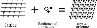
Figure 3: The crystal structure.

	{length, angles}	Bravais lattice
crystal system	{symmetry element}	P	C	I	F
triclinic	$\begin{array}[]{c}\{a\neq b\neq c,\alpha\neq\beta\neq\gamma\}\\ \{\mbox{no symmetry element}\}\end{array}$		-	-	-
monoclinic	$\begin{array}[]{c}\left\{\begin{array}[]{c}a\neq b\neq c\\ \alpha=\gamma=\pi/2,\beta\geq\pi/2\end{array}\right\}\\ \{\mbox{ 1-diad}\}\end{array}$			-	-
orthorhombic	$\begin{array}[]{c}\left\{\begin{array}[]{c}a\neq b\neq c\\ \alpha=\beta=\gamma=\pi/2\end{array}\right\}\\ \{\mbox{mutually orthogonal 3-diad}\}\end{array}$
hexagonal	$\begin{array}[]{c}\left\{\begin{array}[]{c}a=b\neq c\\ \gamma=2\pi/3\end{array}\right\}\\ \{\mbox{1-hexad}\}\end{array}$		-	-	-
trigonal	$\begin{array}[]{c}\left\{\begin{array}[]{c}a=b=c\\ \gamma\neq\pi/3,\pi/2,\cos^{-1}(-{1\over 3})\end{array}\right\}\\ \{\mbox{1-triad}\}\end{array}$		-	-	-
tetragonal	$\begin{array}[]{c}\left\{\begin{array}[]{c}a=b\neq c\\ \alpha=\beta=\gamma=\pi/2\end{array}\right\}\\ \{\mbox{1-tetrad}\}\end{array}$		-		-
cubic	$\begin{array}[]{c}\left\{\begin{array}[]{c}a=b=c\\ \alpha=\beta=\gamma=\pi/2\end{array}\right\}\\ \{\mbox{4-triad}\}\end{array}$		-

Table 1: The Bravais lattices.

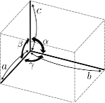
Figure 4: The definitions of the edge lengths and angles in Table 1.

Two crystal lattices belonging to the same crystal system but different sub-classes (that is, two ones in the same row in Table 1) possess the same point group symmetries (that is, the group of symmetry operations that leave at least one lattice point fixed) but different translational symmetries. These, in all, fourteen crystal lattices are known as the Bravais lattices in crystallography. The classification into the fourteen Bravais lattices is further refined into 230 crystal types according to their discrete symmetries called space groups, which are generated by the point group and the group of translational symmetries.

One of the important aspects of such discrete symmetries of a crystal is that they might be used to explain an origin of discrete flavor symmetries [22] in nature (if any), though in the present case in the compactification to six dimensions. Indeed, it has been known for a long time that there are localized [23] 30 hypermultiplets on each symmetric 5-brane (obtained by T-duality in the next section), whose existence is ensured by anomaly cancellation [24, 25], and these hypermultiplets are to be observed as flavors in the warped compactification. It would be interesting to generalize the argument to a similar periodic array of intersecting 5-branes.

Taub-NUT crystals with a highly symmetric structure are very limited. For instance, let us consider cubic lattices with “triads” (that is, symmetry axes of rotations by $120$ degrees) that have 16 positive-charge Taub-NUT’s (Euler number $=24$) as in section 3.3. Then it turns out that the possible type is either of the three shown in Figure 5.

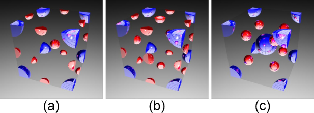
Figure 5: Cubic lattices with triads that have 16 positive-charge Taub-NUT’s. (a) and (b) are of the P type and their subunits are shown there. (c) is of the I type and hence a region larger than a subunit is depicted so that its symmetry may be manifest.

4 T-duality to NS5-brane system

4.1 $O(1,1)$ dual and embedding to heterotic string theory

It is also a well-known fact that the NS5-brane [23, 26] and the Taub-NUT space are related by T-duality [27, 28], which we briefly review here. The NS-NS sector Lagrangian is given in the string frame as

$$2\kappa^{2}{\cal L}_{NSNS} = Ee^{-2\Phi}\left(R+4\partial_{M}\Phi\partial^{M}\Phi-\frac{1}{12}H_{MNP}H^{MNP}\right),$$ (4.1)

where $E$ is the determinant of the vielbein $E^{~{}A}_{M}$, related with the string-frame metric $G_{MN}$ $(M,N=0,\ldots,9)$ as $G_{MN}=E^{~{}A}_{M}E^{~{}B}_{N}\eta_{AB}$. Using the Lorentz invariance, one can cast the vielbein into the form

$$E^{~{}A}_{M} = \left(\begin{array}[]{cc}E^{~{}\alpha}_{\mu}&A_{\mu}\widehat{E}\\ &\\ 0&\widehat{E}\end{array}\right),$$ (4.5)

where $\mu$ ($\alpha$) is a nine-dimensional curved (flat) index. If the metric and all other fields do not depend on $x^{9}$, then decomposing the vielbein as the Lagrangian can be reduced to an $O(1,1)$ sigma model coupled to gravity, an $B$ field, two abelian vector fields and a dilaton, which is invariant under the following transformation [29]:

$${E^{\rm new}}^{~{}\alpha}_{\mu} = E^{~{}\alpha}_{\mu},$$

$${A^{\rm new}}_{\mu} = B_{\mu 9},$$

$${\widehat{E}}^{\rm new} = \widehat{E}^{-1},$$ (4.6)

$${B^{\rm new}}_{\mu\nu} = B_{\mu\nu}-2A_{[\nu}B_{\mu]9},$$

$${B^{\rm new}}_{\mu 9} = A_{\mu},$$

$${\Phi}^{\rm new} = \Phi-\log\widehat{E}.$$

Therefore, starting from a solution of the equations of motion, one can obtain another new solution by applying this transformation to the old one.

We apply the T-duality transformation to the Gibbons-Hawking multi-center metric [8]. If the Gibbons-Hawking metric (3.1) is embedded in eleven dimensions and the $x_{9}$ direction is compactified on $S^{1}$, the metric describes $N$ D6-branes in type IIA theory; this is a string theory analogue of the GPS monopole. Alternatively, we embed (3.1) as a four-dimensional metric in ten dimensions so that the vielbein becomes

$$E_{M}^{~{}A} = \left(\begin{array}[]{ccc}{\bf 1}_{6}&0&0\\ 0&V^{\frac{1}{2}}{\bf 1}_{3}&V^{-\frac{1}{2}}\vec{\omega}\\ 0&0&V^{-\frac{1}{2}}\end{array}\right),$$ (4.10)

while other NS-NS fields are set to zero. Then the $9+1$ decomposition reads

$${E}^{~{}\alpha}_{\mu} = \left(\begin{array}[]{cc}{\bf 1}_{6}&0\\ 0&V^{\frac{1}{2}}{\bf 1}_{3}\end{array}\right),$$ (4.13)

$$A_{\mu} = \left\{\begin{array}[]{ll}0&(\mu=0,\ldots,5),\\ \omega_{x}&(\mu=6),\\ \omega_{y}&(\mu=7),\\ \omega_{z}&(\mu=8),\end{array}\right.$$ (4.18)

$${\widehat{E}} = V^{-\frac{1}{2}},$$ (4.19)

$${B}_{\mu\nu} = 0,$$

$${B}_{\mu 9} = 0,$$

$${\Phi} = 0.$$

Using the transformation rules (4.6), we obtain the T-dual configurations as

$${E^{\rm new}}^{~{}\alpha}_{\mu} = \left(\begin{array}[]{cc}{\bf 1}_{6}&0\\ 0&V^{\frac{1}{2}}{\bf 1}_{3}\end{array}\right),$$ (4.22)

$${A^{\rm new}}_{\mu} = 0,$$

$${\widehat{E}}^{\rm new} = V^{\frac{1}{2}},$$ (4.23)

$${B^{\rm new}}_{\mu\nu} = 0,$$

$${B^{\rm new}}_{\mu 9} = \left\{\begin{array}[]{ll}0&(\mu=0,\ldots,5),\\ \omega_{x}&(\mu=6),\\ \omega_{y}&(\mu=7),\\ \omega_{z}&(\mu=8),\end{array}\right.$$ (4.28)

$${\Phi}^{\rm new} = \frac{1}{2}\log V,$$

or

$$ds_{\rm new}^{2} = \eta_{ij}dx^{i}dx^{j}+V(\vec{x})\delta_{\mu\nu}dx^{\mu}dx^{\nu},$$ (4.29)

$$H^{\rm new}_{\mu\nu 9} = \epsilon^{\rho}_{~{}\mu\nu 9}\partial_{\rho}V(\vec{x}),$$ (4.30)

$$e^{2\Phi^{\rm new}} = V(\vec{x}),$$ (4.31)

where $\epsilon^{\rho}_{~{}\mu\nu 9}$ is normalized to take values $\pm 1$. (4.29)-(4.31) describe $N$ smeared NS5-branes.

It is now obvious that, to obtain the T-dual of the infinite periodic array that we described in section 3, we have only to replace $V$ with (3.10), (3.11) in (4.29)-(4.31), as the T-dual transformation does not depend on the explicit form of $V(\vec{x})$. Thus we obtain a three-dimensional periodic array of, in this case, parallel NS5-branes with one ($x^{9}$) dimension smeared and compactified on a circle. The ${\bf Z}_{2}$ projection (3.13) must also be imposed.

It can also be easily verified that $\Omega^{\rm new}_{\mu\alpha\beta}\pm H^{\rm new}_{\mu\alpha\beta}$, where $\Omega^{\rm new}_{\mu\alpha\beta}$ is the spin connection derived from ${E^{\rm new}}^{~{}\alpha}_{\mu}$, belong to different $SU(2)$ subalgebras of the transverse space holonomy group $SO(4)$. Therefore, the 5-brane system has a hyper-Kähler with torsion geometry, and hence preserves one half the supersymmetries. We can then construct in the standard fashion a supersymmetric heterotic background by identifying some part of the gauge connection to be equal to the generalized spin connection:

$$\Omega^{\rm new}_{\mu\alpha\beta}\pm H^{\rm new}_{\mu\alpha\beta}=(A_{\mu})_{\alpha\beta},$$ (4.32)

where $\alpha,\beta$ on the right hand side are the gauge indices specifying some $SU(2)$ subalgebra of $E_{8}\times E_{8}$ or $SO(32)$.

4.2 T-dual of negative-charge Taub-NUT as heterotic orientifold

The ${\bf Z}_{2}$ identification through every location of the “Atiyah-Hitchin” brane shows that they are orientifold-like objects in heterotic string theory. Another property which supports the identification is their tensions: In the string frame, they have negative ADM energy per unit area as can be easily verified. Of course, this is made possible because they have singularities.

In order to construct a 5-brane system with compact transverse dimensions, we first considered an infinite periodic array of Taub-NUT centers. To make the Gibbons-Hawking potential converge, we were naturally led to introduce negative charge centers as a part of it. Then by T-duality, they turned into branes with negative tension. That is, they need to appear, in this construction, for the transverse space to be compactified. This may be viewed as in accordance with the statement of [4].

Also, in [25, 30], a brane compactification of the $E_{8}\times E_{8}$ heterotic string theory was considered using smeared intersecting 5-branes and the spectrum of fermionic zeromodes was computed. There, some of the intersecting branes were required to have negative tension for a convergent harmonic function of the metric. However, without a microscopic definition of orientifolds in heterotic string, their origin was obscure. The T-dual of (the asymptotic form of) the Atiyah-Hitchin space thus may provide an understanding of such negative tension branes in heterotic string theory (despite the singularity; see next section).

4.3 Discussion: Vortex corrections to the singularity

So far we have considered a system of brane compactification of string theory in the framework of supergravity. In any case, it is not useful when the string coupling is not small, or when the fields vary rapidly compared to the string scale. In this section we discuss the possibility of probing the geometry near the 5-branes by using the sigma-model approach. Of course, heterotic string has no D-brane probes, but one may use them first in type II theories as a systematic means of obtaining a hyper-Kähler geometry (with torsion), and then it may be converted into a heterotic background by the standard embedding.

The three-dimensional $N=4$, $SU(2)$ supersymmetric gauge theory obtained by a dimensional reduction of the four-dimensional $N=2$ gauge theory without hypermultiplets has the Atiyah-Hitchin space as its moduli space [19, 20]. In three dimensions, the $U(1)$ gauge field is dualized to a scalar, so that there are four real scalars whose expectation values parameterize the Coulomb branch moduli space, which must be some hyper-Kähler manifold [31]. To one-loop, the metric is nothing but the negative-charge Taub-NUT that we have used in the Gibbons-Hawking metric. By taking into account the corrections due to monopoles, it was shown that the smooth Atiyah-Hitchin space was singled out from other hyper-Kähler manifolds [19, 20]. Originally, the Atiyah-Hitchin space was discovered [9] as the moduli space of slowly-moving two monopoles in a four-dimensional gauge theory [32]. The appearance of the same moduli space of different gauge theories was explained [33] by considering a D3-NS5-brane system, where the two gauge theories arise as low-energy theories on different branes.

Now suppose that we consider a further dimensional reduction to two dimensions. This is a two-dimensional $(4,4)$ simga model, consisting of a hypermultiplet and a twisted hypermultiplet, both in the adjoint of $SU(2)$. In two dimensions the vector field have no propagating degrees of freedom, and there is no need to dualize anything. The degree of freedom that the three-dimensional dual scalar had is now carried by one of the scalar components of the twisted hypermultiplet. This is essentially the Buscher’s T-duality, and the sigma model is thus expected to describe the T-dual geometry of (in the $SU(2)$ case) the Atiyah-Hitchin space.

This set up was already considered long time ago by Diaconescu and Seiberg [34]. Indeed, in the $SU(2)$ case, they obtained a one-loop (exact) sigma model metric precisely the same as the singular negative-tension brane that we obtained as the T-dual of the negative-charge Taub-NUT. (See also [35].) The relative minus sign in the harmonic function is a reflection of the non-abelian nature of the gauge theory, and in the $U(1)$ case the relative sign is positive, and that corresponds to the ordinary Taub-NUT space. However, unlike in three dimensions where monopoles can exist, there are, at least in the naive sense, no further non-perturbative contribution from vortices in two dimensions on this Coulomb branch; there is no vortices in the reduced two-dimensional theory of the pure $SU(2)$ gauge theory broken to $U(1)$ since $\pi_{1}(SU(2)/U(1))$ is trivial. Still, we note that it has also been known for some time that, in a sense described in [36], the vortex moduli space of the Hitchin system is well-defined and its volume can be computed [36].

Realizing the hyper-Kähler geometry with torsion on the Higgs branch is also interesting. In [37], the smeared 5-brane metric was realized as the Higgs branch moduli space of a $U(1)$ $(4,4)$ sigma model, and it was argued that the world sheet instantons ($=$ vortices) correct the metric into the Poisson re-summed form of the localized 5-brane metric compactified on a circle. It would be interesting if one could generalize this to the negative-tension/Atiyah-Hitchin case. The hyper-Kähler quotient construction for the singular two-monopole moduli space ($=$ the Atiyah-Hitchin space without instanton corrections) is already known [38]. What puzzles us about the result is that, in that case, one needs to start from a flat hyper-Kähler space with an indefinite metric, which would mean that some of the scalars of the sigma model would have to have a wrong-sign kinetic term. The realization on the Higgs branch requires further study.

5 Summary

In this paper we have taken a first step toward realizing warped compactifications using NS5-branes in heterotic string theory. We have first considered the Gibbons-Hawking metric for an infinite periodic array of Taub-NUT’s, and have taken T-duality to obtain a parallel 5-brane system with a compact transverse space having the $SU(2)$ structure, which allowed us to obtain a supersymmetric heterotic 5-brane system via the standard embedding. In order for the Gibbons-Hawking potential to converge, there have been included Taub-NUT centers having a negative NUT charge, which have been identified as the asymptotic forms of the Atiyah-Hitchin metric. This identification has forced us to make a ${\bf Z}_{2}$ projection through the positions of the negative Taub-NUT centers. We have described the convergence condition for the locations of the centers. We have shown that in order for the periodic array to be an approximation of $K_{3}$, the number of the positive charge Taub-NUT’s must be 16 in a unit cell. We have seen some parallels between the periodic array of the Taub-NUT centers and ionic crystals, and structures of the “Taub-NUT crystal” can be similarly classified in terms of the Bravais lattices, of which we have given a brief review.

Since we have used the asymptotic form of the Atiyah-Hitchin metric as a part of the construction, the metric (3.1) with (3.10),(3.11) and (3.3) have singularities near the locations of the negative charges [16, 12], and it only makes sense at distances larger than the charge scale from those charges. Despite the singularities, the compactified/orbifolded infinite periodic array has significance in that (i) it clarifies the origin of negative tension branes in heterotic string theory, and (ii) it basically gives the leading-order behavior of such objects whose corrections from nonperturbative effects might be systematically analyzed by the sigma model approach as we discussed in the text.

Appendix     The Darboux-Halphen system

A.1  The Bianchi IX self-dual metrics

The Bianichi IX metric:

$$ds^{2}=a^{2}b^{2}c^{2}dt^{2}+a^{2}\sigma_{1}^{2}+b^{2}\sigma_{2}^{2}+c^{2}\sigma_{3}^{2}.$$ (A.1)

$a$, $b$ and $c$ are functions of $t$ only. $\sigma_{i}$’s $(i=1,2,3)$ are the Maurer-Cartan 1-forms of $SU(2)$ given by

$$\sigma_{1} = -\sin\psi d\theta+\sin\theta\cos\psi d\phi,$$

$$\sigma_{2} = \cos\psi d\theta+\sin\theta\sin\psi d\phi,$$ (A.2)

$$\sigma_{3} = d\psi+\cos\theta d\phi.$$

If one requires that the spin connection $\omega_{\mu\alpha\beta}$ is self-dual

$$\omega_{\mu\alpha\beta} = +\frac{1}{2}\epsilon_{\alpha\beta}^{~{}~{}~{}\gamma\delta}\omega_{\mu\gamma\delta},$$ (A.3)

then $a$, $b$ and $c$ must satisfy

$$\frac{\dot{a}}{abc} = +\frac{a^{2}-b^{2}-c^{2}}{2bc},$$

$$\frac{\dot{b}}{abc} = +\frac{b^{2}-c^{2}-a^{2}}{2ca},$$ (A.4)

$$\frac{\dot{c}}{abc} = +\frac{c^{2}-a^{2}-b^{2}}{2ab},$$

where  $\dot{}=\frac{d}{dt}$. These conditions are satisfied by the Eguchi-Hanson metric written in the form (A.1). More generally, if one requires that the Riemann curvature tensor is self-dual:

$$R_{\mu\nu\alpha\beta} = +\frac{1}{2}\epsilon_{\alpha\beta}^{~{}~{}~{}\gamma\delta}R_{\mu\nu\gamma\delta},$$ (A.5)

the conditions are [16]

$$\frac{\dot{a}}{abc} = +\frac{a^{2}-b^{2}-c^{2}}{2bc}+\lambda_{a},$$

$$\frac{\dot{b}}{abc} = +\frac{b^{2}-c^{2}-a^{2}}{2ca}+\lambda_{b},$$ (A.6)

$$\frac{\dot{c}}{abc} = +\frac{c^{2}-a^{2}-b^{2}}{2ab}+\lambda_{c}.$$

with

$$\lambda_{a}=\lambda_{b}\lambda_{c},~{}\lambda_{b}=\lambda_{c}\lambda_{a},~{}\lambda_{c}=\lambda_{a}\lambda_{b}.$$ (A.7)

Since (A.7) is invariant under the sign flips

$$a \mapsto +a,$$

$$b \mapsto -b,$$

$$c \mapsto -c,$$

$$\lambda_{a} \mapsto +\lambda_{a},$$

$$\lambda_{b} \mapsto -\lambda_{b},$$

$$\lambda_{c} \mapsto -\lambda_{c}$$ (A.8)

and analogous cyclic generalizations, the consistent values of $\lambda_{i}$’s are essentially $(\lambda_{a},\lambda_{b},\lambda_{c})=(0,0,0)$ or $(1,1,1)$ only. The latter choice corresponds to the cases of the Taub-NUT and the Atiyah-Hitchin spaces.

In the original Atiyah-Hitchin paper [9], the overall signs of all the three equations are flipped, which correspond to an anti-self-dual curvature in our convention. See below for more detail on the Atiyah-Hitchin metric in the original literature.

A.2  The Darboux-Halphen system

This review is based on [14]. As was shown in [9], by a change of variables

$$w_{1}=bc,~{}w_{2}=ca,~{}w_{3}=ab,$$ (A.9)

the equations (A.6) with $\lambda_{a}=\lambda_{b}=\lambda_{c}=1$ reduce to

$$\dot{w}_{1}+\dot{w}_{2}=2w_{1}w_{2},$$

$$\dot{w}_{2}+\dot{w}_{3}=2w_{2}w_{3},$$ (A.10)

$$\dot{w}_{3}+\dot{w}_{1}=2w_{3}w_{1},$$

which is known as the Darboux-Halphen system. As we mentioned in section 2,

$$w_{j}(t) = 2\frac{d}{dt}\log\vartheta_{j+1}(0,i\alpha t)~{}~{}~{}(j=1,2,3),$$ (A.11)

($\alpha>0$) is a solution [14, 15]. This can be shown by using the composition formula of the theta functions and the fact that the theta functions fulfill the heat equation.

The original Atiyah-Hitchin solution can be written in this form as

$$w^{AH}_{j}(\eta) = -2\frac{d}{d\eta}\log\vartheta_{j+1}(0,-i\pi\eta)~{}~{}~{}(j=1,2,3),$$ (A.12)

while the solution obtained by Gibbons-Manton [16] is

$$w^{GM}_{j}(\eta) = -2\frac{d}{d\eta}\log\vartheta_{j+1}(0,-2i\pi\eta)~{}~{}~{}(j=1,2,3).$$ (A.13)

As we remarked at the end of the last subsection, (A.12) has extra minus signs since they satisfy the anti-self-dual equations (see (A.14)). Comparisons of the solutions are made in the next section.

A.3  Comparison with solutions in the literature

In this section we derive eqs.(A.12) and (A.13).

A.3.1  Atiyah-Hitchin’s original solution

Let us first consider (A.12). In [9], a set of solutions are given to the Darboux-Halphen system

$$w^{\prime}_{1}+w^{\prime}_{2} = -2w_{1}w_{2},$$

$$w^{\prime}_{2}+w^{\prime}_{3} = -2w_{2}w_{3},$$ (A.14)

$$w^{\prime}_{3}+w^{\prime}_{1} = -2w_{3}w_{1},$$

which corresponds to $a$, $b$ and $c$ satisfying

$$\frac{a^{\prime}}{abc} = -\frac{a^{2}-b^{2}-c^{2}}{2bc}-1,$$

$$\frac{b^{\prime}}{abc} = -\frac{b^{2}-c^{2}-a^{2}}{2ca}-1,$$ (A.15)

$$\frac{c^{\prime}}{abc} = -\frac{c^{2}-a^{2}-b^{2}}{2ab}-1,$$

where the prime ^′ denotes $\frac{d}{d\eta}$. The metric is assumed to have the form (A.1) with the ‘radial’ coordinate $\eta$ replaced instead of $t$. The relations between $w_{j}$’s and $a,b,c$ are (A.9). The solutions are given in terms of the coordinate $\beta$ such that

$$\frac{d\beta}{d\eta} = u^{2},$$ (A.16)

where $u=u(\beta)$ is a function of $\beta$ satisfying

$$\frac{d^{2}u}{d\beta^{2}}+\frac{u^{2}}{4\sin^{2}\beta}=0.$$ (A.17)

A solution to (A.17) is explicitly

$$u(\beta) = (2\sin\beta)^{\frac{1}{2}}K(\sin\frac{\beta}{2}),$$ (A.18)

where

$$K(k) = \int_{0}^{\frac{\pi}{2}}\frac{d\phi}{(1-k^{2}\sin^{2}\phi)^{\frac{1}{2}}}$$ (A.19)

is the complete elliptic integral of the first kind. According to [9], we set

$$w_{2}^{AH} = -u\frac{du}{d\beta}+\frac{u^{2}}{2}\cot\beta,$$

$$w_{3}^{AH} = -u\frac{du}{d\beta}+\frac{u^{2}}{2}\frac{1}{\sin\beta},$$ (A.20)

$$w_{1}^{AH} = -u\frac{du}{d\beta}-\frac{u^{2}}{2}\frac{1}{\sin\beta}.$$

Using (A.18), we have

$$w_{2}^{AH} = -\frac{d}{d\eta}\log K(\sin\frac{\beta}{2}),$$

$$w_{3}^{AH} = -\frac{d}{d\eta}\log\left(\sin\frac{\beta}{2}~{}K(\sin\frac{\beta}{2})\right),$$ (A.21)

$$w_{1}^{AH} = -\frac{d}{d\eta}\log\left(\cos\frac{\beta}{2}~{}K(\sin\frac{\beta}{2})\right).$$

The elliptic theta functions and the elliptic integrals are known to be related as

$$K(k) = \frac{\pi}{2}\vartheta_{3}(0,\tau(k))^{2},$$

$$\sqrt{1-k^{2}}K(k) = \frac{\pi}{2}\vartheta_{4}(0,\tau(k))^{2},$$ (A.22)

$$kK(k) = \frac{\pi}{2}\vartheta_{2}(0,\tau(k))^{2},$$

where the modulus $\tau(k)$ is given by

$$\tau(k)=i\frac{K(\sqrt{1-k^{2}})}{K(k)}.$$ (A.23)

Let us consider $w_{2}^{AH}$. Using these equations, we can further rewrite the expression of $w_{2}^{AH}$ as

$$w_{2}^{AH} = -2\frac{d}{d\eta}\log\vartheta_{3}\left(0,i\frac{K(\cos\frac{\beta}{2})}{K(\sin\frac{\beta}{2})}\right).$$ (A.24)

Using the differential relations among the elliptic functions one can show the relation [14]

$$\frac{d}{d\beta}\tau({\textstyle\sin\frac{\beta}{2}}) = \frac{-i\pi}{2\sin\beta~{}K(\sin\frac{\beta}{2})^{2}}.$$ (A.25)

The right hand side is equal to $\frac{-i\pi}{u(\beta)^{2}}$. Comparing (A.25) with (A.16), we find

$$\frac{d\tau({\textstyle\sin\frac{\beta}{2}})}{d\beta}=-i\pi\frac{d\eta}{d\beta}.$$ (A.26)

If we choose the arbitrary integration constant to be $0$, we have

$$\tau({\textstyle\sin\frac{\beta}{2}}) = -\pi i\eta,$$ (A.27)

and

$$w_{2}^{AH} = -2\frac{d}{d\eta}\log\vartheta_{3}(0,-i\pi\eta).$$ (A.28)

Expressions for $w_{3}^{AH}$ and $w_{1}^{AH}$ can be obtained similarly.

A remark is in order here. Since the imaginary part of the elliptic modulus of must be positive, (A.27) implies that $\eta$ takes its value from $-\infty$ to $0$, which is puzzling if it is regarded as a radial coordinate. Since the system of equations (A.14) is invariant under the simultaneous sign flips $w_{j}\mapsto-w_{j}$ and $\eta\mapsto-\eta$, one might wonder if

$$w_{j}^{AH} \stackrel{{\scriptstyle?}}{{=}} -2\frac{d}{d\eta}\log\vartheta_{j+1}(0,+i\pi\eta)$$ (A.29)

also work. They do not, however, because, although (A.29) still solves (A.14), $a^{2}$, $b^{2}$ and $c^{2}$ derived from (A.29) with (A.9) turn out to be negative. This problem can be cured by either changing the relations (A.9) to ones with minus sign: $w_{1}=-bc,$ etc., or replacing (A.14) with the self-dual equations (A.10) without minus signs on the right hand sides; in any case one is forced to modify some of the assumptions made in [9]. We have numerically checked that (A.12) (and not (A.29)) is correct by Mathematica.

While, of course, these complications are not essential, we adopted (A.10) instead of (A.14) in the text for a simpler notation with less minus signs. Note that, unlike $\eta$, the coordinate $t$ in (A.11) takes its value from $0$ to $+\infty$.

A.3.2  Gibbons-Manton’s solution

In [16], the radial coordinate was chosen so that the Bianchi IX metric took the following form:

$$ds^{2} = \frac{b^{2}}{\tilde{r}^{2}}d\tilde{r}^{2}+a^{2}\sigma_{1}^{2}+b^{2}\sigma_{2}^{2}+c^{2}\sigma_{3}^{2}.$$ (A.30)

$a$, $b$ and $c$ which solve

$$-\frac{\tilde{r}}{b}\frac{da}{d\tilde{r}} = -\frac{a^{2}-b^{2}-c^{2}}{2bc}-1,$$

$$-\frac{\tilde{r}}{b}\frac{db}{d\tilde{r}} = -\frac{b^{2}-c^{2}-a^{2}}{2ca}-1,$$ (A.31)

$$-\frac{\tilde{r}}{b}\frac{dc}{d\tilde{r}} = -\frac{c^{2}-a^{2}-b^{2}}{2ab}-1$$

give an anti-self-dual metric. The solution was similarly given in terms of $w_{j}=w^{GM}_{j}$ ($j=1,2,3$) (A.9) as

$$w_{2}^{GM} = -\tilde{r}\sin\beta\frac{d\tilde{r}}{d\beta},$$

$$w_{3}^{GM} = -\tilde{r}\sin\beta\frac{d\tilde{r}}{d\beta}+\frac{\tilde{r}^{2}}{2}(1-\cos\beta),$$ (A.32)

$$w_{1}^{GM} = -\tilde{r}\sin\beta\frac{d\tilde{r}}{d\beta}-\frac{\tilde{r}^{2}}{2}(1-\cos\beta)$$

with

$$\tilde{r} = 2K\left(\sin\frac{\beta}{2}\right).$$ (A.33)

To derive (A.13), we change variables so that the metric takes the form (A.1):

$$abc\;d\tilde{\eta}=-\frac{b}{\tilde{r}}d\tilde{r}.$$ (A.34)

$\tilde{\eta}$ is the new radial coordinate. Then (A.33) implies that

$$\frac{d\tilde{\eta}}{d\beta} = \frac{1}{2u(\beta)^{2}},$$ (A.35)

where $u(\beta)$ is the function (A.18). On the other hand, $w^{GM}_{2}$ can be similarly written as

$$w^{GM}_{2} = -\frac{d}{d\tilde{\eta}}\log K\left(\sin\frac{\beta}{2}\right)$$ (A.36)

$$= -2\frac{d}{d\tilde{\eta}}\log\vartheta_{3}\left(0,i\frac{K(\cos\frac{\beta}{2})}{K(\sin\frac{\beta}{2})}\right).$$ (A.37)

Comparing (A.25) with (A.35), we have in this case

$$\tau\left(\sin\frac{\beta}{2}\right) = -2\pi i\tilde{\eta},$$ (A.38)

and therefore

$$w_{2}^{GM} = -2\frac{d}{d\tilde{\eta}}\log\vartheta_{3}(0,-2i\pi\tilde{\eta}).$$ (A.39)

The proofs for $w_{3}^{GM}$ and $w_{1}^{GM}$ are also straightforward.

We have shown that the value of $\alpha$ (A.11) for Gibbons-Manton’s solution is $2\pi$. Plugging $\alpha=2\pi$ into (2.16), we find agreement with the asymptotic metric obtained in [16].

References

-
[1]
G. Gibbons, ”Aspects of Supergravity Theories”, in Aguilla, del F., Azcarrage,
A. and Ibanez, L. eds., Supersymmetry, Supergravity and Related Topics,
World Scientific (1985).
B. de Wit, D. J. Smit and N. D. Hari Dass, Nucl. Phys. B 283, 165 (1987).
J. M. Maldacena and C. Nunez, Int. J. Mod. Phys. A 16, 822 (2001) [arXiv:hep-th/0007018]. -
[2]
L. Randall and R. Sundrum,
Phys. Rev. Lett. 83 (1999) 3370
[arXiv:hep-ph/9905221].
L. Randall and R. Sundrum, Phys. Rev. Lett. 83 (1999) 4690 [arXiv:hep-th/9906064]. - [3] H. L. Verlinde, Nucl. Phys. B 580, 264 (2000) [arXiv:hep-th/9906182].
- [4] S. B. Giddings, S. Kachru and J. Polchinski, Phys. Rev. D 66, 106006 (2002) [arXiv:hep-th/0105097].
- [5] S. Kachru, R. Kallosh, A. D. Linde and S. P. Trivedi, Phys. Rev. D 68, 046005 (2003) [arXiv:hep-th/0301240].
- [6] A. Hanany and B. Kol, JHEP 0006, 013 (2000) [arXiv:hep-th/0003025].
-
[7]
B. S. Acharya, F. Benini and R. Valandro,
JHEP 0702 (2007) 018
[arXiv:hep-th/0607223].
T. Banks and K. van den Broek, JHEP 0703 (2007) 068 [arXiv:hep-th/0611185]. - [8] G. W. Gibbons and S. W. Hawking, Phys. Lett. B 78, 430 (1978).
- [9] M. F. Atiyah and N. J. Hitchin, “The Geometry And Dynamics Of Magnetic Monopoles. M. B. Porter Lectures.” Princeton University Press (1988).
- [10] M. Cvetic, G. W. Gibbons, H. Lu and C. N. Pope, Annals Phys. 310, 265 (2004) [arXiv:hep-th/0111096].
- [11] K. Rutlidge, “Infinite-Centre Gibbons-Hawking Metrics, Applied to Gravitational Instantons and Monopoles.” Doctoral thesis, Durham University (2010). Available at Durham E-Theses Online: http://etheses.dur.ac.uk/383/
- [12] A. Sen, JHEP 9709, 001 (1997) [arXiv:hep-th/9707123].
- [13] S. J. . Gates, C. M. Hull and M. Rocek, Nucl. Phys. B 248, 157 (1984).
- [14] Y. Ohyama, Osaka Journal of Mathematics 32(2), 431-450 (1995).
- [15] A. Hanany and B. Pioline, JHEP 0007, 001 (2000) [arXiv:hep-th/0005160].
- [16] G. W. Gibbons and N. S. Manton, Nucl. Phys. B 274, 183 (1986).
- [17] E. J. Weinberg and P. Yi, Phys. Rept. 438, 65 (2007) [arXiv:hep-th/0609055].
- [18] T. Eguchi, P. B. Gilkey and A. J. Hanson, Phys. Rept. 66, 213 (1980).
- [19] N. Seiberg and E. Witten, arXiv:hep-th/9607163.
- [20] N. Dorey, V. V. Khoze, M. P. Mattis, D. Tong and S. Vandoren, Nucl. Phys. B 502, 59 (1997) [arXiv:hep-th/9703228].
- [21] M. A. Walton, Phys. Rev. D 37, 377 (1988).
- [22] H. Ishimori, T. Kobayashi, H. Ohki, Y. Shimizu, H. Okada and M. Tanimoto, Prog. Theor. Phys. Suppl. 183, 1 (2010) [arXiv:1003.3552 [hep-th]] and references therein.
-
[23]
C. G. . Callan, J. A. Harvey and A. Strominger,
Nucl. Phys. B 359, 611 (1991).
C. G. . Callan, J. A. Harvey and A. Strominger, Nucl. Phys. B 367, 60 (1991). -
[24]
J. M. Izquierdo and P. K. Townsend,
Nucl. Phys. B 414 (1994) 93
[arXiv:hep-th/9307050].
J. D. Blum and J. A. Harvey, Nucl. Phys. B 416 (1994) 119 [arXiv:hep-th/9310035].
J. Mourad, Nucl. Phys. B 512 (1998) 199 [arXiv:hep-th/9709012].
H. Imazato, S. Mizoguchi and M. Yata, Mod. Phys. Lett. A 26 (2011) 1453 [arXiv:1010.1640 [hep-th]]. -
[25]
T. Kimura and S. Mizoguchi,
JHEP 1004 (2010) 028
[arXiv:0912.1334 [hep-th]].
- [26] S. J. Rey, Phys. Rev. D 43, 526 (1991).
- [27] R. Gregory, J. A. Harvey and G. W. Moore, Adv. Theor. Math. Phys. 1, 283 (1997) [arXiv:hep-th/9708086].
- [28] B. Andreas, G. Curio and D. Lust, JHEP 9810, 022 (1998) [arXiv:hep-th/9807008].
-
[29]
J. Maharana and J. H. Schwarz,
Nucl. Phys. B 390, 3 (1993)
[arXiv:hep-th/9207016].
A. Sen, Nucl. Phys. B 404, 109 (1993) [arXiv:hep-th/9207053]. - [30] T. Kimura and S. Mizoguchi, Class. Quant. Grav. 27, 185023 (2010) [arXiv:0905.2185 [hep-th]].
- [31] L. Alvarez-Gaume and D. Z. Freedman, Commun. Math. Phys. 80, 443 (1981).
- [32] N. S. Manton, Phys. Lett. B 110, 54 (1982).
- [33] A. Hanany and E. Witten, Nucl. Phys. B 492, 152 (1997) [arXiv:hep-th/9611230].
- [34] D. E. Diaconescu and N. Seiberg, JHEP 9707 (1997) 001 [arXiv:hep-th/9707158].
- [35] A. V. Smilga, “Low dimensional sisters of Seiberg-Witten effective theory,” arXiv:hep-th/0403294.
- [36] G. W. Moore, N. Nekrasov and S. Shatashvili, Commun. Math. Phys. 209, 97 (2000) [arXiv:hep-th/9712241].
- [37] D. Tong, JHEP 0207, 013 (2002) [arXiv:hep-th/0204186].
- [38] G. W. Gibbons and P. Rychenkova, Commun. Math. Phys. 186, 585 (1997) [arXiv:hep-th/9608085].