A simple linear response closure approximation for slow dynamics of a multiscale system with linear coupling

Abstract.

Many applications of contemporary science involve multiscale dynamics, which are typically characterized by the time and space scale separation of patterns of motion, with fewer slowly evolving variables and much larger set of faster evolving variables. This time-space scale separation causes direct numerical simulation of the evolution of the dynamics to be computationally expensive, due both to the large number of variables and the necessity to choose a small discretization time step in order to resolve the fast components of dynamics. In this work we propose a simple method of determining the closed model for slow variables alone, which requires only a single computation of appropriate statistics for the fast dynamics with a certain fixed state of the slow variables. The method is based on the first-order Taylor expansion of the averaged coupling term with respect to the slow variables, which can be computed using the linear fluctuation-dissipation theorem. We show that, with simple linear coupling in both slow and fast variables, this method produces quite comparable statistics to what is exhibited by a complete two-scale model. The main advantage of the method is that it applies even when the statistics of the full multiscale model cannot be simulated due to computational complexity, which makes it practical for real-world large scale applications.

1. Introduction

Multiscale dynamics are common in applications of contemporary science, such as geophysical science and climate change prediction [15, 16, 9, 24]. Multiscale dynamics are typically characterized by the time and space scale separation of patterns of motion, with (typically) fewer slowly evolving variables and much larger set of faster evolving variables. This time-space scale separation causes direct numerical simulation of the evolution of the dynamics be computationally expensive, due both to the large number of variables and the necessity to choose a small discretization time step in order to resolve the fast components of dynamics.

In the climate change science the situation is further complicated by the fact that climate is characterized by the long-term statistics of the slow variables, which, under small changes of parameters (such as the solar radiation forcing, greenhouse gas content, etc) change over even longer time scale than the motion of the slow variables themselves. In this situation, where long-term statistics of the slow motion patterns need to be captured, the direct forward time integration of the most comprehensive global circulation models (GCM) is subject to enormous computational expense.

As a more computationally feasible alternative to direct forward time integration of the complete multiscale model, it has long been recognized that, if a closed simplified model for the slow variables alone is available, one could use this closed slow-variable model instead to simulate the statistics of the slow variables. Numerous closure schemes were developed for multiscale dynamical systems [10, 13, 20, 23, 21, 22], which are all based on the averaging principle over the fast variables [25, 32, 33]. Some of the methods (such as those in [20, 23, 21, 22]) replace the fast nonlinear dynamics with suitable stochastic processes [34] or conditional Markov chains [10], while others [13] provide direct closure by suitable tabulation and curve fitting. However, it seems that all these approaches require either extensive computations to produce a closed model (for example,[10, 13] require multiple simulations of fast variables alone with different fixed states of slow variables), or somewhat ad hoc determination of closure coefficients by matching areas under the time correlation functions [20, 23, 21, 22].

In this work we propose a simple method of determining the closed model for slow variables alone, which requires only a single computation of appropriate statistics for the fast dynamics with a certain fixed state of the slow variables. The method is based on the first-order Taylor expansion of the averaged coupling term with respect to the slow variables, which, as we show, can be computed using the linear fluctuation-dissipation theorem [1, 2, 3, 4, 6, 5, 7, 8, 19, 26]. We show through the computations with the appropriately rescaled two-scale Lorenz 96 model [4] that, with simple linear coupling in both slow and fast variables, this method produces quite comparable statistics to what is exhibited by the slow variables of the complete two-scale Lorenz model. The main advantage of the method is its simplicity and easiness of implementation, partly due to the fact that the fast dynamics need not be explicitly known (that is, the fast dynamics can be provided as a “black-box” algorithm), and the parameters of the closed model for the slow variables are determined from the appropriate statistics of the fast variables for a given fixed state of the slow variables. Additionally, the method can be applied even when the statistics for slow variables of the full multiscale model are not available due to computational expense.

The manuscript is structured as follows. In Section 2 we outline the theoretical grounds for the algorithm. In Section 3 we describe the two-scale Lorenz model [13, 17, 18], appropriately rescaled so that the means and variances of both the fast and slow variables are near zero and one, respectively [4]. Section 4 contains the results of numerical experiments with both the two-scale Lorenz model and the reduced set of equations for slow variables only, comparing various statistics of the time series. Section 5 summarizes the results of this work.

2. The linear response closure approximation

Consider a two-scale system of differential equations of the form

(2.1) $$\frac{\mathrm{d}\boldsymbol{x}}{\mathrm{d}t}=\boldsymbol{F}(\boldsymbol{x},\boldsymbol{y}),\qquad\frac{\mathrm{d}\boldsymbol{y}}{\mathrm{d}t}=\boldsymbol{G}(\boldsymbol{x},\boldsymbol{y}),$$

where $\boldsymbol{x}=\boldsymbol{x}(t)\in\mathbb{R}^{N_{x}}$ are the slow variables, $\boldsymbol{y}=\boldsymbol{y}(t)\in\mathbb{R}^{N_{y}}$ are the fast variables, and $\boldsymbol{F}$ and $\boldsymbol{G}$ are $N_{x}$ and $N_{y}$ vector-valued functions of $\boldsymbol{x}$ and $\boldsymbol{y}$, respectively. Here and below, we assume that the fast variables $\boldsymbol{y}$ are “unresolved”, that is, the computation of the dynamics for $\boldsymbol{y}$ requires such a small time discretization step, that the direct computation of (2.1) for long time intervals is practically infeasible. We also assume that the dynamics for $\boldsymbol{y}$ are fast enough for the system in (2.1) to be approximated by the averaged dynamics for $\boldsymbol{x}$, given by

(2.2) $$\frac{\mathrm{d}\boldsymbol{x}}{\mathrm{d}t}=\langle\boldsymbol{F}\rangle(\boldsymbol{x}),\qquad\langle\boldsymbol{F}\rangle(\boldsymbol{x})=\int_{\mathbb{R}^{N_{y}}}\boldsymbol{F}(\boldsymbol{x},\boldsymbol{z})\,\mathrm{d}\mu_{\boldsymbol{x}}(\boldsymbol{z}),$$

for finite times (for a more detailed description of the averaging formalism, see [2, 4, 25, 32, 33]). Above, $\mu_{\boldsymbol{x}}$ is the invariant probability measure of the limiting fast dynamics given by

(2.3) $$\frac{\mathrm{d}\boldsymbol{z}}{\mathrm{d}\tau}=\boldsymbol{G}(\boldsymbol{x},\boldsymbol{z}),$$

where the solution is given by the flow $\boldsymbol{z}(\tau)=\phi_{\boldsymbol{x}}^{\tau}\boldsymbol{z}_{0}$, while $\boldsymbol{x}$ is a fixed constant parameter for (2.3) and, consequently, $\mu_{\boldsymbol{x}}$. Below we assume that $\langle\boldsymbol{F}\rangle(\boldsymbol{x})$ varies smoothly with respect to $\boldsymbol{x}$ (it is known that for stochastically driven systems this property is generic, and for deterministic dynamics this happens when $\mu_{\boldsymbol{x}}$ is an SRB measure [12, 28, 29, 27, 35]). Under the ergodicity assumption for $\mu_{\boldsymbol{x}}$, one can replace the measure average with time average:

(2.4) $$\langle\boldsymbol{F}\rangle(\boldsymbol{x})=\lim_{r\to\infty}\frac{1}{r}\int_{0}^{r}\boldsymbol{F}(\boldsymbol{x},\boldsymbol{z}(\tau))\,\mathrm{d}\tau,$$

where $\boldsymbol{z}(\tau)$ is a long-term trajectory of (2.3).

While suitable multiscale methods exist (see [11] and references therein) where the computation of the average in (2.4) is performed relatively rarely, even that might not be computationally feasible in complex multiscale systems with many fast variables. For the purpose of this work, here we assume that the computation of (2.3) is practically feasible only for a single choice of the constant parameter $\boldsymbol{x}=\boldsymbol{x}^{*}$, where $\boldsymbol{x}^{*}$ is a suitable point, in the vicinity of which the motion occurs, such as the mean state of the original dynamics in (2.1), or a nearby state. A poor man’s approach in this case is to compute the approximate average with respect to $\mu_{\boldsymbol{x}^{*}}$, which is a zero order approximation:

(2.5) $$\langle\boldsymbol{F}\rangle(\boldsymbol{x})=\int_{\mathbb{R}^{N_{y}}}\boldsymbol{F}(\boldsymbol{x},\boldsymbol{z})\,\mathrm{d}\mu_{\boldsymbol{x}^{*}}(\boldsymbol{z})+\mathcal{O}(\|\boldsymbol{x}-\boldsymbol{x}^{*}\|).$$

Here, one has to compute the time average in (2.4) only once, for the time series of (2.3) corresponding to $\boldsymbol{x}=\boldsymbol{x}^{*}$. However, as recently found in [4], this approximation may fail to capture the chaotic properties of the slow variables in (2.1). Here we propose the following first order correction:

(2.6) $$\begin{split}\langle\boldsymbol{F}\rangle(\boldsymbol{x})&=\int_{\mathbb{R}^{N_{y}}}\boldsymbol{F}(\boldsymbol{x},\boldsymbol{z})\,\mathrm{d}\mu_{\boldsymbol{x}^{*}}(\boldsymbol{z})+\\ +&\left[\int_{\mathbb{R}^{N_{y}}}\boldsymbol{F}(\boldsymbol{x},\boldsymbol{z})\,\mathrm{d}\mu_{\boldsymbol{x}^{*}}^{\prime}(\boldsymbol{z})\right](\boldsymbol{x}-\boldsymbol{x}^{*})+\mathcal{O}(\|\boldsymbol{x}-\boldsymbol{x}^{*}\|^{2}),\end{split}$$

where $\mu_{\boldsymbol{x}^{*}}^{\prime}$ is the derivative of $\mu_{\boldsymbol{x}}$ with respect to $\boldsymbol{x}$, computed at the point $\boldsymbol{x}=\boldsymbol{x}^{*}$. It is shown in [4] that the average of $\boldsymbol{F}$ with respect to $\mu_{\boldsymbol{x}^{*}}^{\prime}$ can be computed as the corresponding infinite time linear response to infinitesimal perturbation of $\boldsymbol{x}$ (for details on the linear response theory, see [1, 2, 3, 4, 6, 5, 7, 8, 19, 26] and references therein):

(2.7) $$\int_{\mathbb{R}^{N_{y}}}\boldsymbol{F}(\boldsymbol{x},\boldsymbol{z})\,\mathrm{d}\mu_{\boldsymbol{x}^{*}}^{\prime}(\boldsymbol{z})=\int_{0}^{\infty}\int_{\mathbb{R}^{N_{y}}}\frac{\partial\boldsymbol{F}}{\partial\boldsymbol{y}}(\boldsymbol{x},\phi_{\boldsymbol{x}^{*}}^{s}\boldsymbol{z})\boldsymbol{T}_{\boldsymbol{x}^{*},\boldsymbol{z}}^{s}\frac{\partial\boldsymbol{G}}{\partial\boldsymbol{x}}(\boldsymbol{x}^{*},\boldsymbol{z})\,\mathrm{d}\mu_{\boldsymbol{x}^{*}}(\boldsymbol{z})\,\mathrm{d}s,$$

where $\partial\boldsymbol{F}/\partial\boldsymbol{y}$ is the Jacobian with respect to the second argument of $\boldsymbol{F}$, and $\boldsymbol{T}_{\boldsymbol{x}^{*},\boldsymbol{z}}^{\tau}$ is the tangent map of (2.3):

(2.8) $$\boldsymbol{T}_{\boldsymbol{x}^{*},\boldsymbol{z}}^{\tau}=\frac{\partial}{\partial\boldsymbol{z}}\phi_{\boldsymbol{x}^{*}}^{\tau}\boldsymbol{z}.$$

Under the assumption of ergodicity of $\mu_{\boldsymbol{x}^{*}}$, (2.7) can be written as the integral of the time autocorrelation function, which is computed along a single long-time trajectory $\boldsymbol{z}^{*}(\tau)$ of (2.3) with $\boldsymbol{x}=\boldsymbol{x}^{*}$:

(2.9) $$\begin{split}\int_{\mathbb{R}^{N_{y}}}&\boldsymbol{F}(\boldsymbol{x},\boldsymbol{z})\,\mathrm{d}\mu_{\boldsymbol{x}^{*}}^{\prime}(\boldsymbol{z})=\\ =&\int_{0}^{\infty}\left[\lim_{r\to\infty}\int_{0}^{r}\frac{\partial\boldsymbol{F}}{\partial\boldsymbol{y}}(\boldsymbol{x},\boldsymbol{z}^{*}(\tau+s))\boldsymbol{T}_{z^{*}(\tau)}^{s}\frac{\partial\boldsymbol{G}}{\partial\boldsymbol{x}}(\boldsymbol{x}^{*},\boldsymbol{z}^{*}(\tau))\,\mathrm{d}\tau\right]\,\mathrm{d}s,\end{split}$$

which is also done only once along the same long-term trajectory of (2.3), as for the time average in (2.5) (for practical purposes, it can be assumed that the time autocorrelation function decays sufficiently fast to replace the improper integral from zero to infinity with a proper integral up to a sufficiently long time). While formally valid, the above formula can be unsuitable for practical computation due to the fact that usually the limiting fast dynamics in (2.3) are strongly chaotic and mixing with large positive Lyapunov exponents. The presence of large positive Lyapunov exponents causes numerical instability in the computation of the tangent map $\boldsymbol{T}$ of (2.3) for long response times, and, as a result, the infinite-time linear response in (2.9) cannot be computed. Below we consider the special setting for (2.1) with linear coupling (which is common in geophysical sciences), and use the quasi-Gaussian linear response approximation [1, 2, 3, 6, 5, 7, 8, 19] for the practical computation of (2.9).

2.1. Special case with linear coupling

Here we consider the special setting of (2.1) with linear coupling between $\boldsymbol{x}$ and $\boldsymbol{y}$:

(2.10) $$\boldsymbol{F}(\boldsymbol{x},\boldsymbol{y})=\boldsymbol{f}(\boldsymbol{x})+\boldsymbol{L}_{y}\boldsymbol{y},\qquad\boldsymbol{G}(\boldsymbol{x},\boldsymbol{y})=\boldsymbol{g}(\boldsymbol{y})+\boldsymbol{L}_{x}\boldsymbol{x},$$

where $\boldsymbol{f}$ and $\boldsymbol{g}$ are nonlinear vector functions of $\boldsymbol{x}$ and $\boldsymbol{y}$, respectively, and $\boldsymbol{L}_{x}$ and $\boldsymbol{L}_{y}$ are constant matrices of suitable sizes. For this simplified setting, observe that $\partial\boldsymbol{G}/\partial\boldsymbol{x}=\boldsymbol{L}_{x}$, $\partial\boldsymbol{F}/\partial\boldsymbol{y}=\boldsymbol{L}_{y}$, and, therefore, the approximate averaged system is given by

(2.11a) $$\frac{\mathrm{d}\boldsymbol{x}}{\mathrm{d}t}=\boldsymbol{f}(\boldsymbol{x})+\boldsymbol{L}_{y}\boldsymbol{\bar{z}}^{*}+\boldsymbol{L}_{y}\boldsymbol{R}^{*}\boldsymbol{L}_{x}(\boldsymbol{x}-\boldsymbol{x}^{*}),$$

(2.11b) $$\boldsymbol{\bar{z}}^{*}=\lim_{r\to\infty}\frac{1}{r}\int_{0}^{r}\boldsymbol{z}^{*}(\tau)\,\mathrm{d}\tau,$$

(2.11c) $$\boldsymbol{R}^{*}=\int_{0}^{\infty}\left[\lim_{r\to\infty}\frac{1}{r}\int_{0}^{r}\boldsymbol{T}_{\boldsymbol{z}^{*}(\tau)}^{s}\,\mathrm{d}\tau\right]\,\mathrm{d}s,$$

where $\boldsymbol{z}(t)$ is the solution of the fast limiting system

(2.12) $$\frac{\mathrm{d}\boldsymbol{z}}{\mathrm{d}t}=\boldsymbol{g}(\boldsymbol{z})+\boldsymbol{L}_{x}\boldsymbol{x}$$

with $\boldsymbol{x}$ specified as a constant parameter, and $\boldsymbol{z}^{*}(t)$ corresponds to $\boldsymbol{x}=\boldsymbol{x}^{*}$. The formula in (2.11c) is usually unsuitable for direct numerical computation due to rapidly growing Lyapunov exponents at fast scales. Instead, one can use the quasi-Gaussian linear response approximation, where (2.11c) becomes the integral of the time autocorrelation function under the assumption of the Gaussian invariant measure for (2.12). With linear coupling, the measure-averaged linear response formula (2.7) becomes

(2.13) $$\int_{\mathbb{R}^{N_{y}}}\boldsymbol{F}(\boldsymbol{x},\boldsymbol{z})\,\mathrm{d}\mu_{\boldsymbol{x}^{*}}^{\prime}(\boldsymbol{z})=\boldsymbol{L}_{y}\left(\int_{0}^{\infty}\int_{\mathbb{R}^{N_{y}}}\boldsymbol{T}_{\boldsymbol{x}^{*},\boldsymbol{z}}^{s}\,\mathrm{d}\mu_{\boldsymbol{x}^{*}}(\boldsymbol{z})\,\mathrm{d}s\right)\boldsymbol{L}_{x}.$$

Now, the Gaussian probability density is given by

(2.14) $$p_{G}^{*}(\boldsymbol{z})=(2\pi)^{-\frac{N_{y}}{2}}\det\boldsymbol{\Sigma}^{*-\frac{1}{2}}\exp\left(-\frac{1}{2}(\boldsymbol{z}-\boldsymbol{\bar{z}}^{*})^{T}\boldsymbol{\Sigma}^{*-1}(\boldsymbol{z}-\boldsymbol{\bar{z}}^{*})\right),$$

where $\boldsymbol{\Sigma}^{*}$ is the long-time covariance matrix of (2.12), computed at the point $\boldsymbol{x}^{*}$:

(2.15) $$\boldsymbol{\Sigma}^{*}=\lim_{r\to\infty}\frac{1}{r}\int_{0}^{r}(\boldsymbol{z}^{*}(\tau)-\boldsymbol{\bar{z}}^{*})(\boldsymbol{z}^{*}(\tau)-\boldsymbol{\bar{z}}^{*})^{T}\,\mathrm{d}\tau.$$

Recalling that $\boldsymbol{T}_{\boldsymbol{x}^{*},\boldsymbol{z}}^{s}=\partial\phi_{\boldsymbol{x}^{*}}^{s}\boldsymbol{z}/\partial\boldsymbol{z}$ and replacing $\,\mathrm{d}\mu_{\boldsymbol{x}^{*}}(\boldsymbol{z})=p_{G}^{*}(\boldsymbol{z})\,\mathrm{d}\boldsymbol{z}$, we obtain, after integration by parts over $\boldsymbol{z}$,

(2.16) $$\int_{\mathbb{R}^{N_{y}}}\boldsymbol{F}(\boldsymbol{x},\boldsymbol{z})\,\mathrm{d}\mu_{\boldsymbol{x}^{*}}^{\prime}(\boldsymbol{z})=-\boldsymbol{L}_{y}\left(\int_{0}^{\infty}\int_{\mathbb{R}^{N_{y}}}\phi_{\boldsymbol{x}^{*}}^{s}\boldsymbol{z}\frac{\partial p_{G}^{*}(\boldsymbol{z})}{\partial\boldsymbol{z}}\,\mathrm{d}\boldsymbol{z}\,\mathrm{d}s\right)\boldsymbol{L}_{x}.$$

Computing the derivative of (2.14) with respect to $\boldsymbol{z}$, we obtain

(2.17) $$\int_{\mathbb{R}^{N_{y}}}\boldsymbol{F}(\boldsymbol{x},\boldsymbol{z})\,\mathrm{d}\mu_{\boldsymbol{x}^{*}}^{\prime}(\boldsymbol{z})=\boldsymbol{L}_{y}\left(\int_{0}^{\infty}\int_{\mathbb{R}^{N_{y}}}\phi_{\boldsymbol{x}^{*}}^{s}\boldsymbol{z}(\boldsymbol{z}-\boldsymbol{\bar{z}}^{*})^{T}p_{G}^{*}(\boldsymbol{z})\,\mathrm{d}\boldsymbol{z}\,\mathrm{d}s\right)\boldsymbol{\Sigma}^{*-1}\boldsymbol{L}_{x}.$$

Switching back to time-averaging, we obtain

(2.18) $$\begin{split}\int_{\mathbb{R}^{N_{y}}}\boldsymbol{F}(\boldsymbol{x},\boldsymbol{z})&\,\mathrm{d}\mu_{\boldsymbol{x}^{*}}^{\prime}(\boldsymbol{z})=\\ =\boldsymbol{L}_{y}&\int_{0}^{\infty}\left[\lim_{r\to\infty}\frac{1}{r}\int_{0}^{r}\boldsymbol{z}^{*}(\tau+s)(\boldsymbol{z}^{*}(\tau)-\boldsymbol{\bar{z}}^{*})^{T}\,\mathrm{d}\tau\right]\,\mathrm{d}s\;\boldsymbol{\Sigma}^{*-1}\boldsymbol{L}_{x},\end{split}$$

and, therefore, $\boldsymbol{R}^{*}$ in (2.11a) can now be computed as

(2.19) $$\boldsymbol{R}^{*}=\int_{0}^{\infty}\left[\lim_{r\to\infty}\frac{1}{r}\int_{0}^{r}\boldsymbol{z}^{*}(\tau+s)(\boldsymbol{z}^{*}(\tau)-\boldsymbol{\bar{z}}^{*})^{T}\,\mathrm{d}\tau\right]\,\mathrm{d}s\;\boldsymbol{\Sigma}^{*-1}.$$

For details, see [1, 2, 3, 6, 5, 7, 8, 19]).

For even better precision of the linear response computation, one can also use the blended linear response approximation [6, 5, 7, 8], however, in this work we do not implement it, as it is shown that for the model and regimes considered, the quasi-Gaussian approximation is already quite precise.

Even with the linear coupling, the function $\boldsymbol{\bar{z}}(\boldsymbol{x})$ (the dependence of the mean state of (2.12) on $\boldsymbol{x}$) is not generally linear. Thus, the validity of the linear approximation in (2.11a) depends on the influence (or lack thereof) of the nonlinearity of the function $\boldsymbol{\bar{z}}(\boldsymbol{x})$. While rigorous estimates of the validity of the linear approximation in (2.11a) can hardly be provided in general case, here, instead, we try to justify it by comparing the fast limiting system in (2.12) to the Ornstein-Uhlenbeck process [31]. Consider an Ornstein-Uhlenbeck process of the form

(2.20) $$\frac{\mathrm{d}\boldsymbol{z}}{\mathrm{d}\tau}=-\boldsymbol{\Gamma}(\boldsymbol{z}-\boldsymbol{m})+\boldsymbol{L}_{x}\boldsymbol{x}+\boldsymbol{\sigma}\frac{\mathrm{d}\boldsymbol{W}_{\tau}}{\mathrm{d}\tau},$$

where $\boldsymbol{m}$ is a constant $N_{y}$-vector, $\boldsymbol{\Gamma}$ is a constant $N_{y}\times N_{y}$ positive-definite matrix, $\boldsymbol{W}_{t}$ is a $K$-dimensional Wiener process, $\boldsymbol{\sigma}$ is a constant $N_{y}\times K$ matrix, and $\boldsymbol{x}$ is, as in (2.12), is a constant parameter. Then, it is easy to see that the difference between the statistical mean states of (2.20) corresponding to $\boldsymbol{x}$ and $\boldsymbol{x}^{*}$ is

(2.21) $$\boldsymbol{\bar{z}}_{OU}-\boldsymbol{\bar{z}}_{OU}^{*}=\boldsymbol{\Gamma}^{-1}\boldsymbol{L}_{x}(\boldsymbol{x}-\boldsymbol{x}^{*}),$$

which is valid for $(\boldsymbol{x}-\boldsymbol{x}^{*})$ of an arbitrary norm. At the same time, by the regression theorem [26], the time correlation function of (2.20) with $\boldsymbol{x}=\boldsymbol{x}^{*}$ is given by

(2.22) $$\langle\boldsymbol{z}_{OU}^{*}(t+s)(\boldsymbol{z}_{OU}^{*}(t)-\boldsymbol{\bar{z}}_{OU}^{*})^{T}\rangle=\exp(-s\boldsymbol{\Gamma})\boldsymbol{\Sigma}_{OU}^{*},$$

where $\boldsymbol{\Sigma}_{OU}^{*}$ is the covariance matrix of the Ornstein-Uhlenbeck process in (2.20) for $\boldsymbol{x}=\boldsymbol{x}^{*}$. Thus, according to (2.19), the infinite-time linear response operator for (2.20) is computed as

(2.23) $$\boldsymbol{R}_{OU}^{*}=\int_{0}^{\infty}\exp(-s\boldsymbol{\Gamma})\,\mathrm{d}s=\boldsymbol{\Gamma}^{-1}.$$

By comparing (2.23) with (2.21), one can see that, for the Ornstein-Uhlenbeck process, the quasi-Gaussian linear response formula in (2.19) is exact for an arbitrarily large perturbation $(\boldsymbol{x}-\boldsymbol{x}^{*})$. Hence, if the nonlinear process in (2.12) behaves statistically similarly to the Ornstein-Uhlenbeck process in (2.20), the averaged system in (2.11a) can be expected to behave statistically similarly to the slow part of (2.10). Below we numerically test the approximation for slow variables in the special setting with linear coupling using the two-scale Lorenz model [1, 2, 4, 10, 13, 17].

3. The two-scale Lorenz model

Here we choose the two-scale forced damped Lorenz model [1, 2, 4, 10, 13, 17] for the computational study of the dynamical properties of a two-scale slow-fast process with generic features of climate-weather systems, such as the presence of linearly unstable waves, strong nonlinearity, forcing, dissipation, chaos and mixing. The two-scale forced damped Lorenz model is given by

(3.1a) $$\dot{x}_{i}=x_{i-1}(x_{i+1}-x_{i-2})-x_{i}+F_{x}-\frac{\lambda_{y}}{J}\sum_{j=1}^{J}y_{i,j},$$

(3.1b) $$\dot{y}_{i,j}=\frac{1}{\varepsilon}\left[y_{i,j+1}(y_{i,j-1}-y_{i,j+2})-y_{i,j}+F_{y}\right]+\frac{\lambda_{x}}{\varepsilon}x_{i},$$

where $1\leq i\leq N_{x}$, $1\leq j\leq J$. The following notations are adopted above:

• $\boldsymbol{x}$ is the set of the slow variables of size $N_{x}$. The following periodic boundary conditions hold for $\boldsymbol{x}$: $x_{i+N_{x}}=x_{i}$;

• $\boldsymbol{y}$ is the set of the fast variables of size $N_{y}=N_{x}J$ where $J$ is a positive integer. The following boundary conditions hold for $\boldsymbol{y}$: $y_{i+N_{x},j}=y_{i,j}$ and $y_{i,j+J}=y_{i+1,j}$;

• $F_{x}$ and $F_{y}$ are the constant forcing parameters;

• $\lambda_{x}$ and $\lambda_{y}$ are the coupling parameters;

• $\varepsilon$ is the time scale separation parameter.

Originally in [10, 13, 17] there was no constant forcing $F$ term in the equation for $\boldsymbol{x}$-variables in (3.1), however, in its absence the behavior of the $\boldsymbol{y}$-variables is strongly dissipative [1, 2]. Here, as in [2], we add a constant forcing $F_{y}$ in the right-hand side of the second equation in (3.1) to induce the strongly chaotic behavior of the $\boldsymbol{y}$-variables with large positive Lyapunov exponents.

3.1. Rescaled Lorenz model

In the Lorenz model (3.1), $F_{x}$ and $F_{y}$ regulate the chaos and mixing of the $\boldsymbol{x}$ and $\boldsymbol{y}$ variables, respectively [1, 2, 4]. However, the mean state and mean energy are also affected by the changes in forcing, which affects the mean and energy trends in coupling for the fixed coupling parameters. To adjust the effect of coupling independently of forcing, here we rescale the Lorenz model as in [19]. Consider the uncoupled Lorenz model

(3.2) $$\frac{\mathrm{d}}{\mathrm{d}t}x_{i}=x_{i-1}(x_{i+1}-x_{i-2})-x_{i}+F$$

with the same periodic boundary conditions as above [18]. Observe that the long term statistical mean state $\bar{x}$ and the standard deviation $\beta$ in (3.2) are the same for all $x_{i}$ due to the translational invariance. Now, we rescale $\boldsymbol{x}$ and $t$ as

(3.3) $$x_{i}=\bar{x}+\beta\hat{x}_{i},\quad t=\frac{\tau}{\beta},$$

where the new variables $\boldsymbol{\hat{x}}$ have zero mean state and unit standard deviation. In the rescaled variables, the Lorenz model becomes

(3.4) $$\frac{\mathrm{d}}{\mathrm{d}\tau}\hat{x}_{i}=\hat{x}_{i-1}(\hat{x}_{i+1}-\hat{x}_{i-2})+\frac{1}{\beta}\left[\bar{x}(\hat{x}_{i+1}-\hat{x}_{i-2})-\hat{x}_{i}\right]+\frac{F-\bar{x}}{\beta^{2}},$$

where $\bar{x}$ and $\beta$ are, of course, the functions of $F$. In addition to setting the mean state and variance of $\hat{x}_{i}$ to zero and one, respectively, due to the time rescaling the autocorrelation functions of $\boldsymbol{z}$ acquire roughly identical time scaling for any $F$ (for details, see [19]). Here, we similarly rescale the two-scale Lorenz model from (3.1):

(3.5a) $$\dot{x}_{i}=x_{i-1}(x_{i+1}-x_{i-2})+\frac{1}{\beta_{x}}\left(\bar{x}(x_{i+1}-x_{i-2})-x_{i}\right)+\frac{F_{x}-\bar{x}}{\beta_{x}^{2}}-\frac{\lambda_{y}}{J}\sum_{j=1}^{J}y_{i,j},$$

(3.5b) $$\begin{split}\dot{y}_{i,j}=\frac{1}{\varepsilon}\bigg{[}y_{i,j+1}(y_{i,j-1}-y_{i,j+2})+\frac{1}{\beta_{y}}\left(\bar{y}(y_{i,j-1}-y_{i,j+2})-y_{i,j}\right)+\\ +\frac{F_{y}-\bar{y}}{\beta_{y}^{2}}\bigg{]}+\frac{\lambda_{x}}{\varepsilon}x_{i},\end{split}$$

where $\bar{x}$, $\bar{y}$, $\beta_{x}$ and $\beta_{y}$ are the long term means and standard deviations of the corresponding uncoupled system in (3.2) with either $F_{x}$ or $F_{y}$ set as a constant forcing. In the rescaled Lorenz model (3.5), the values of $F_{x}$ and $F_{y}$ do not significantly affect the mean state, mean energy and the time scale for both the slow variables $\boldsymbol{x}$ and fast variables $\boldsymbol{y}$, and mostly regulate the mixing and non-Gaussianity of the probability distributions of the long-term time series.

The Lorenz model (3.5) represents the setting with linear coupling as in (2.10), with $\boldsymbol{f}$, $\boldsymbol{g}$, $\boldsymbol{L}_{x}$ and $\boldsymbol{L}_{y}$ given by

(3.6a) $$f_{i}(\boldsymbol{x})=x_{i-1}(x_{i+1}-x_{i-2})+\frac{1}{\beta_{x}}\left(\bar{x}(x_{i+1}-x_{i-2})-x_{i}\right)+\frac{F_{x}-\bar{x}}{\beta_{x}^{2}},$$

(3.6b) $$\begin{split}g_{i,j}(\boldsymbol{y})=\frac{1}{\varepsilon}\bigg{[}y_{i,j+1}(y_{i,j-1}-y_{i,j+2})+\frac{1}{\beta_{y}}\left(\bar{y}(y_{i,j-1}-y_{i,j+2})-y_{i,j}\right)+\\ +\frac{F_{y}-\bar{y}}{\beta_{y}^{2}}\bigg{]},\end{split}$$

(3.6c) $$\boldsymbol{L}_{x}=\frac{\lambda_{x}}{\varepsilon}\boldsymbol{L}^{T},\qquad\boldsymbol{L}_{y}=-\frac{\lambda_{y}}{J}\boldsymbol{L},\qquad\boldsymbol{L}_{i,(j,k)}=\delta_{ij}.$$

Now, one can immediately see that for the Lorenz model in (3.5), the limiting system in (2.3) is given by

(3.7) $$\frac{\mathrm{d}\boldsymbol{z}}{\mathrm{d}\tau}=\boldsymbol{g}(\boldsymbol{z})+\frac{\lambda_{x}}{\varepsilon}\boldsymbol{L}^{T}\boldsymbol{x},$$

while the approximate averaged system around the point $\boldsymbol{x}^{*}$ is given by

(3.8) $$\frac{\mathrm{d}\boldsymbol{x}}{\mathrm{d}t}=\boldsymbol{f}(\boldsymbol{x})-\frac{\lambda_{y}}{J}\boldsymbol{L}\boldsymbol{\bar{z}}^{*}-\frac{\lambda_{x}\lambda_{y}}{\varepsilon J}\boldsymbol{L}\boldsymbol{R}^{*}\boldsymbol{L}^{T}(\boldsymbol{x}-\boldsymbol{x}^{*}).$$

Above, the parameter $\varepsilon$ in the denominator suggests that the first-order correction term is of order $\varepsilon^{-1}$, which is misleading, because $\boldsymbol{R}^{*}$ scales proportionally to $\varepsilon$ (since it is the integral of the time autocorrelation function with rate of decay proportional to $\varepsilon^{-1}$). For simplicity of computation, for the Lorenz model we rescale the fast limiting dynamics by $\varepsilon$ to bring the time scale to order 1 since the scaling parameter $\varepsilon$ is known explicitly, which yields

(3.9) $$\frac{\mathrm{d}\boldsymbol{z}}{\mathrm{d}\tau}=\varepsilon\boldsymbol{g}(\boldsymbol{z})+\lambda_{x}\boldsymbol{L}^{T}\boldsymbol{x},$$

for the fast limiting dynamics for fixed $\boldsymbol{x}$, while for the averaged dynamics we obtain

(3.10) $$\frac{\mathrm{d}\boldsymbol{x}}{\mathrm{d}t}=\boldsymbol{f}(\boldsymbol{x})-\frac{\lambda_{y}}{J}\boldsymbol{L}\boldsymbol{\bar{z}}^{*}-\frac{\lambda_{x}\lambda_{y}}{J}\boldsymbol{L}\boldsymbol{R}^{*}\boldsymbol{L}^{T}(\boldsymbol{x}-\boldsymbol{x}^{*}),$$

where $\boldsymbol{R}^{*}$ is computed from the time series of (3.9) using the quasi-Gaussian approximation in (2.19).

4. Numerical experiments

Here we present a numerical study of the proposed approximation for slow dynamics, applied to the rescaled Lorenz model in (3.5). We compare the statistical properties of the slow variables for the three following systems:

1. The complete rescaled Lorenz system from (3.5);

2. The approximation for slow dynamics alone from (3.10);

3. The poor man’s version of (3.10) with the first-order correction term $\boldsymbol{R}^{*}$ set to zero (further referred to as the “zero-order” system).

The fixed parameter $\boldsymbol{x}^{*}$ for the computation of $\boldsymbol{R}^{*}$ was set to the long-term mean state $\boldsymbol{\bar{x}}$ of (3.5) (in practical situations, a rough estimate could be used). The quasi-Gaussian approximation in (2.19) is used to compute the first order correction term $\boldsymbol{R}^{*}$. While it is practically impossible to compute the improper integrals in (2.19) for infinite upper limit, in practice we use sufficiently long (but finite) limits of integration. In particular, for all computational results presented below, the correction term $\boldsymbol{R}^{*}$ is computed numerically as

(4.1) $$\boldsymbol{R}^{*}=\frac{1}{T_{av}}\int_{0}^{T_{corr}}\int_{0}^{T_{av}}\boldsymbol{z}^{*}(\tau+s)(\boldsymbol{z}^{*}(\tau)-\boldsymbol{\bar{z}}^{*})^{T}\,\mathrm{d}\tau\,\mathrm{d}s\;\boldsymbol{\Sigma}^{*-1},$$

where the averaging time window $T_{av}$ equals 10000 time units, while the correlation time window $T_{corr}$ equals 50 time units (it was observed that the time autocorrelation function in (4.1) decays essentially to zero within the 50 time-unit window for all studied regimes). The mean state $\boldsymbol{\bar{z}}^{*}$ and the covariance matrix $\boldsymbol{\Sigma}^{*}$ are also computed by time-averaging with the same averaging window of 10000 time units.

Due to translational invariance of the studied models, the statistics are invariant with respect to the index shift for the variables $x_{i}$. For diagnostics, we monitor the following long-term statistical quantities of $x_{i}$:

1. The probability density functions (PDF), computed by bin-counting. A PDF gives the most complete information about the one-point statistics of $x_{i}$, as it shows the statistical distribution of $x_{i}$ in the phase space.

2. The time autocorrelation functions $\langle x_{i}(t)x_{i}(t+s)\rangle$, where the time average is over $t$, normalized by the variance $\langle x_{i}^{2}\rangle$ (so that it always starts with 1).

3. The time cross-correlation functions $\langle x_{i}(t)x_{i+1}(t+s)\rangle$, also normalized by the variance $\langle x_{i}^{2}\rangle$.

4. The energy autocorrelation function

   $$K(s)=\frac{\langle x_{i}^{2}(t)x_{i}^{2}(t+s)\rangle}{\langle x_{i}^{2}\rangle^{2}+2\langle x_{i}(t)x_{i}(t+s)\rangle^{2}}.$$

   This energy autocorrelation function measures the non-Gaussianity of the process (it is identically 1 for all $s$ if the process is Gaussian, such as the Ornstein-Uhlenbeck process). For details, see [22].

The success (or failure) of the proposed approximation of the slow dynamics depends on several factors. First, as the quasi-Gaussian linear response formula is used for the computation of $\boldsymbol{R}^{*}$, the precision will be affected by the non-Gaussianity of the fast dynamics. Second, it depends how linearly the mean state $\boldsymbol{\bar{z}}$ for the fast variables depends on the slow variables $\boldsymbol{x}$. Here we observe the limitations of the proposed approximation by studying a variety of dynamical regimes of the rescaled Lorenz model in (3.5). The following dynamical regimes are studied:

• $N_{x}=20$, $J=4$ (so that $N_{y}=80$). Thus, the number of the fast variables is four times greater than the number of the slow variables.

• $\varepsilon=0.01$. The time scale separation of two orders of magnitude is consistent with typical real-world geophysical processes (for example, the annual and diurnal cycles of the Earth’s atmosphere).

• $\lambda_{x}=\lambda_{y}=0.3,0.4$. These values of coupling are chosen so that they are neither too weak, nor too strong (although 0.3 is weaker, and 0.4 is stronger). Recall that the standard deviations of both $x_{i}$ and $y_{i,j}$ variables are approximately 1, and, thus, the contribution to the right-hand side from coupled variables is weaker than the self-contribution, but still of the same order.

• $F_{x}=6,16$. The slow forcing $F_{x}$ adjusts the chaos and mixing properties of the slow variables, and in this work it is set to a weakly chaotic regime $F_{x}=6$, and strongly chaotic regime $F_{x}=16$.

• $F_{y}=8,12$. The fast forcing adjusts the chaos and mixing properties of the fast variables. Here the value of $F_{y}$ is chosen so that the fast variables are either moderately chaotic for $F_{y}=8$, or more strongly chaotic for $F_{y}=12$.

In Figure 4.1 we show the probability density functions and time autocorrelation functions for the limiting fast dynamics in (3.9), with the parameters $N_{x}=20$, $N_{y}=80$, $F_{x}=6$, $\lambda_{x}=\lambda_{y}=0.3$, and two values of the fast forcing: $F_{y}=8$ and $F_{y}=12$. Observe that the PDFs are not Gaussian (although close to it), and have nonzero skewness. The time autocorrelation functions decay slower for $F_{y}=8$ and faster for $F_{y}=12$, indicating slower and faster mixing, respectively. In other regimes, these PDFs and autocorrelation functions look very similar to what is presented in Figure 4.1.

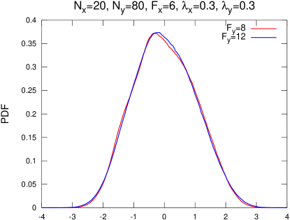
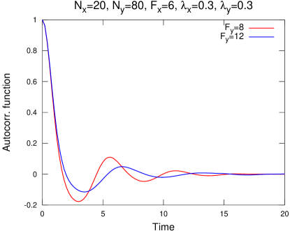
Figure 4.1. The probability density functions and time autocorrelation functions of the limiting fast dynamics in (3.9) for $F_{x}=6$, and $\lambda_{x}=\lambda_{y}=0.3$.

Another point we would like to emphasize before presenting the results of the computational study, is that the matrices $\boldsymbol{R}^{*}$ and, consequently, $\boldsymbol{L}\boldsymbol{R}\boldsymbol{L}^{T}$ in (3.10) are not diagonal. In Figure 4.2 we display both $\boldsymbol{R}^{*}$ and $\boldsymbol{L}\boldsymbol{R}\boldsymbol{L}^{T}$ for the dynamical regime with $F_{x}=6$, $F_{y}=8$, and $\lambda_{x}=\lambda_{y}=0.4$ (only the central columns of $\boldsymbol{R}^{*}$ and $\boldsymbol{L}\boldsymbol{R}\boldsymbol{L}^{T}$ are displayed with diagonal elements corresponding to zero horizontal coordinates of the plots, as both matrices are translation-invariant). Observe that there are significant off-diagonal entries in both matrices. Both $\boldsymbol{R}^{*}$ and $\boldsymbol{L}\boldsymbol{R}\boldsymbol{L}^{T}$ are positive-definite in the presented regime (the lowest eigenvalues of their symmetric parts are $6.314\cdot 10^{-2}$ and $0.8814$, respectively), and, as a result, the linear correction term in (3.10) causes damping effect on the reduced dynamics (for more details about chaotic properties of reduced dynamics, see [4]). For other regimes, the matrices are similar to the presented regime (that is, substantial off-diagonal entries are present), and we do not display those here.

Figure 4.2. The matrices $\boldsymbol{R}^{*}$ (left) and $\boldsymbol{L}\boldsymbol{R}^{*}\boldsymbol{L}^{T}$ (right) of the reduced dynamics in (3.10) for $F_{x}=6$, $F_{y}=8$, and $\lambda_{x}=\lambda_{y}=0.4$. Only a single column of each matrix is displayed with its diagonal element corresponding to zero horizontal coordinate, as the matrices are translation-invariant.

4.1. Probability density functions of the slow dynamics

In Figures 4.3 and 4.4 we show the probability density functions of the slow dynamics for the full two-scale Lorenz model, the reduced closed model for the slow variables alone in (3.10), and its poor man’s zero order version without the linear correction term. Observe that for the more weakly coupled regimes with $\lambda_{x}=\lambda_{y}=0.3$ the PDFs look rather similar, however, it can be seen that the reduced model with the correction term reproduces the PDFs much closer to those of the full two-scale Lorenz model, than the zero-order model. In the more strongly coupled regime with $\lambda_{x}=\lambda_{y}=0.4$ the situation tilts even more in favor of the reduced model with linear correction term in (3.10): observe that for the weakly chaotic regime with $F_{x}=6$ the PDFs of the full two-scale Lorenz model have three sharp peaks, indicating strong non-Gaussianity. The reduced model in (3.10) reproduces these peaks, while its zero-order version fails.

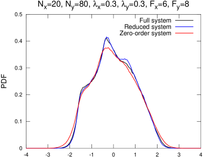
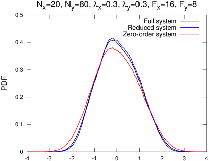
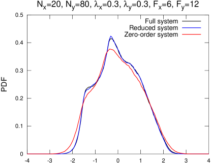
Figure 4.3. PDFs, $\lambda_{x}=\lambda_{y}=0.3$.

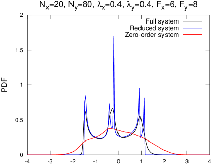
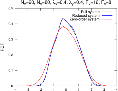
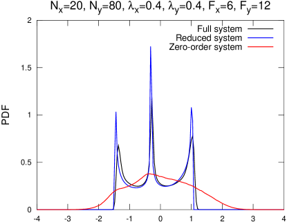
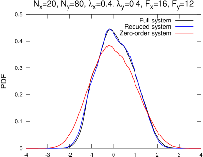
Figure 4.4. PDFs, $\lambda_{x}=\lambda_{y}=0.4$.

In addition, in Table 4.1 we show the $L_{2}$-errors in PDFs between the full two-scale Lorenz model and the two reduced models. Observe that, generally, the reduced system with the linear correction term in (3.10) produces more precise results than its poor man’s version without the correction term.

$\lambda_{x,y}=0.3$, $F_{y}=8$ $\lambda_{x,y}=0.3$, $F_{y}=12$ Red. Z.O. $F_{x}=6$ $5.036\cdot 10^{-3}$ $1.165\cdot 10^{-2}$ $F_{x}=16$ $5.593\cdot 10^{-3}$ $1.469\cdot 10^{-2}$ Red. Z.O. $F_{x}=6$ $2.581\cdot 10^{-3}$ $1.576\cdot 10^{-2}$ $F_{x}=16$ $2.71\cdot 10^{-3}$ $1.818\cdot 10^{-2}$

$\lambda_{x,y}=0.4$, $F_{y}=8$ $\lambda_{x,y}=0.4$, $F_{y}=12$ Red. Z.O. $F_{x}=6$ $0.1022$ $8.857\cdot 10^{-2}$ $F_{x}=16$ $3.725\cdot 10^{-3}$ $2.703\cdot 10^{-2}$ Red. Z.O. $F_{x}=6$ $9.28\cdot 10^{-2}$ $0.1113$ $F_{x}=16$ $5.885\cdot 10^{-3}$ $3.209\cdot 10^{-2}$

Table 4.1. $L_{2}$-errors between the PDFs of the slow variables of the full two-scale Lorenz model and the two reduced models. Notations: “Red.” stands for “Reduced” (that is, (3.10)), and “Z.O.” stands for “Zero-order”, the poor man’s version of (3.10).

4.2. Time autocorrelation functions of the slow dynamics

In Figures 4.5 and 4.6 we show the time autocorrelation functions of the slow dynamics for the full two-scale Lorenz model, the reduced closed model for the slow variables alone in (3.10), and its poor man’s zero order version without the linear correction term. Observe that for the more weakly coupled regimes with $\lambda_{x}=\lambda_{y}=0.3$ the time autocorrelation functions look similar, yet the reduced model with the correction term reproduces the time autocorrelation functions more precisely than the zero-order model. In the more strongly coupled regime with $\lambda_{x}=\lambda_{y}=0.4$ the difference between the reduced model in (3.10) and its poor man’s zero-order version is even more drastic: observe that for the weakly chaotic regime with $F_{x}=6$ the time autocorrelation functions of the full two-scale Lorenz model do not exhibit decay (indicating very weak mixing), and the reduced model in (3.10) reproduces the autocorrelation functions of the full two-scale Lorenz model rather well, while its zero-order version fails.

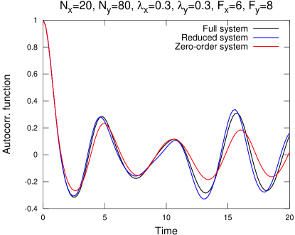
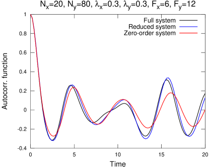
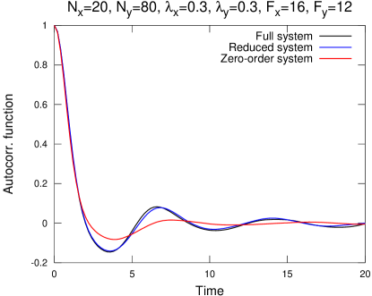
Figure 4.5. Time autocorrelation functions, $\lambda_{x}=\lambda_{y}=0.3$.

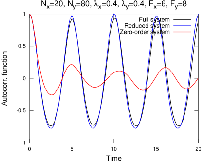
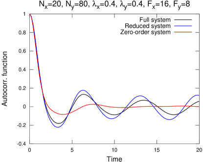
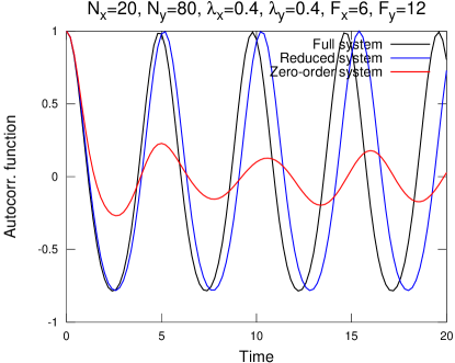
Figure 4.6. Time autocorrelation functions, $\lambda_{x}=\lambda_{y}=0.4$.

In addition, in Table 4.2 we show the $L_{2}$-errors in time autocorrelation functions (for the correlation time interval of 20 time units, as in Figures 4.5 and 4.6) between the full two-scale Lorenz model and the two reduced models. Observe that, generally, the reduced system with the linear correction term in (3.10) produces more precise results than its poor man’s version without the correction term.

$\lambda_{x,y}=0.3$, $F_{y}=8$ $\lambda_{x,y}=0.3$, $F_{y}=12$ Av. Z.O. $F_{x}=6$ $5.841\cdot 10^{-2}$ $0.1211$ $F_{x}=16$ $4.079\cdot 10^{-2}$ $5.342\cdot 10^{-2}$ Av. Z.O. $F_{x}=6$ $6.539\cdot 10^{-2}$ $0.1572$ $F_{x}=16$ $1.559\cdot 10^{-2}$ $7.396\cdot 10^{-2}$

$\lambda_{x,y}=0.4$, $F_{y}=8$ $\lambda_{x,y}=0.4$, $F_{y}=12$ Av. Z.O. $F_{x}=6$ $5.538\cdot 10^{-2}$ $0.3677$ $F_{x}=16$ $8.534\cdot 10^{-2}$ $0.1355$ Av. Z.O. $F_{x}=6$ $0.2981$ $0.3986$ $F_{x}=16$ $4.835\cdot 10^{-2}$ $0.1482$

Table 4.2. $L_{2}$-errors between the time autocorrelation functions of the slow variables of the full two-scale Lorenz model and the two reduced models. Notations: “Red.” stands for “Reduced” (that is, (3.10)), and “Z.O.” stands for “Zero-order”, the poor man’s version of (3.10).

4.3. Time cross-correlation functions

In Figures 4.7 and 4.8 we show the time cross-correlation functions of the slow dynamics for the full two-scale Lorenz model, the reduced closed model for the slow variables alone in (3.10), and its poor man’s zero order version without the linear correction term. Observe that for the more weakly coupled regimes with $\lambda_{x}=\lambda_{y}=0.3$ the time cross-correlation functions look similar, however, it is seen that the reduced model with the correction term reproduces the time cross-correlation functions more precisely than the zero-order model. In the more strongly coupled regime with $\lambda_{x}=\lambda_{y}=0.4$, the reduced model in (3.10) becomes much more precise than its poor man’s zero-order version: here, for the weakly chaotic regime with $F_{x}=6$ the time cross-correlation functions of the full two-scale Lorenz model do not exhibit decay (indicating very weak mixing), and the reduced model in (3.10) reproduces the cross-correlation functions of the full two-scale Lorenz model rather well, while its zero-order version fails.

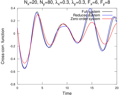
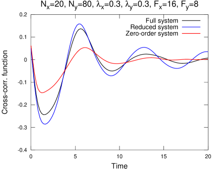
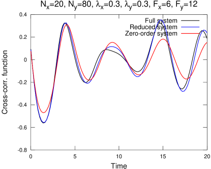
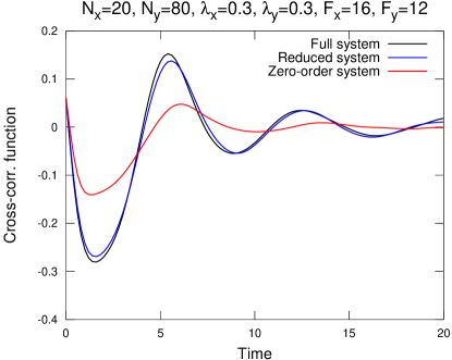
Figure 4.7. Time cross-correlation functions, $\lambda_{x}=\lambda_{y}=0.3$.

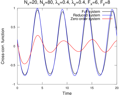
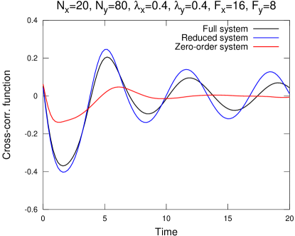
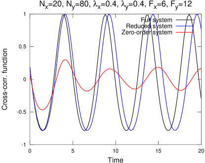
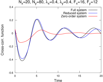
Figure 4.8. Time cross-correlation functions, $\lambda_{x}=\lambda_{y}=0.4$.

In addition, in Table 4.3 we show the $L_{2}$-errors in time cross-correlation functions (for the correlation time interval of 20 time units, as in Figures 4.7 and 4.8) between the full two-scale Lorenz model and the two reduced models. Observe that, generally, the reduced system with the linear correction term in (3.10) produces more precise results than its poor man’s version without the correction term.

$\lambda_{x,y}=0.3$, $F_{y}=8$ $\lambda_{x,y}=0.3$, $F_{y}=12$ Av. Z.O. $F_{x}=6$ $6.825\cdot 10^{-2}$ $0.1437$ $F_{x}=16$ $0.1094$ $0.2134$ Av. Z.O. $F_{x}=6$ $6.838\cdot 10^{-2}$ $0.1799$ $F_{x}=16$ $3.687\cdot 10^{-2}$ $0.2548$

$\lambda_{x,y}=0.4$, $F_{y}=8$ $\lambda_{x,y}=0.4$, $F_{y}=12$ Av. Z.O. $F_{x}=6$ $5.313\cdot 10^{-2}$ $0.3666$ $F_{x}=16$ $0.1258$ $0.3232$ Av. Z.O. $F_{x}=6$ $0.3137$ $0.3942$ $F_{x}=16$ $6.953\cdot 10^{-2}$ $0.3321$

Table 4.3. $L_{2}$-errors between the time cross-correlation functions of the slow variables of the full two-scale Lorenz model and the two reduced models. Notations: “Red.” stands for “Reduced” (that is, (3.10)), and “Z.O.” stands for “Zero-order”, the poor man’s version of (3.10).

4.4. Energy autocorrelation functions

In Figures 4.9 and 4.10 we show the energy autocorrelation functions of the slow dynamics for the full two-scale Lorenz model, the reduced closed model for the slow variables alone in (3.10), and its poor man’s zero order version without the linear correction term. Observe that for the more weakly coupled regimes with $\lambda_{x}=\lambda_{y}=0.3$ the energy autocorrelation functions look similar, although the reduced model with the correction term reproduces the energy autocorrelation functions more precisely than the zero-order model. In the more strongly coupled regime with $\lambda_{x}=\lambda_{y}=0.4$, the reduced model in (3.10) is much more precise than its poor man’s zero-order version: here, for the weakly chaotic regime with $F_{x}=6$ the energy autocorrelation functions of the full two-scale Lorenz model is significantly sub-Gaussian, and the reduced model in (3.10) reproduces the sub-Gaussianity of the energy autocorrelation functions of the full two-scale Lorenz model rather well, while its zero-order version fails.

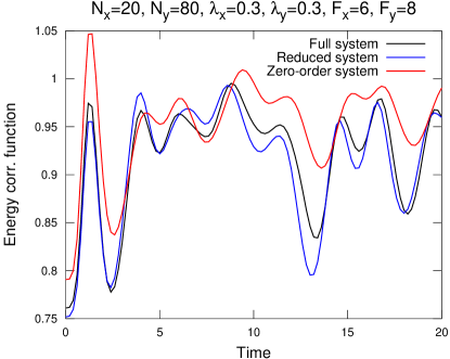
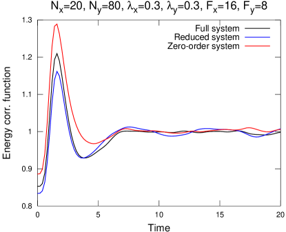
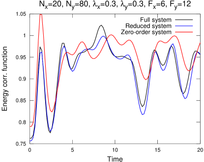
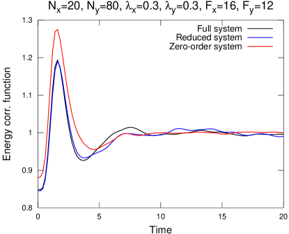
Figure 4.9. Energy autocorrelation functions, $\lambda_{x}=\lambda_{y}=0.3$.

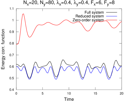
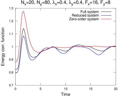
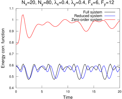
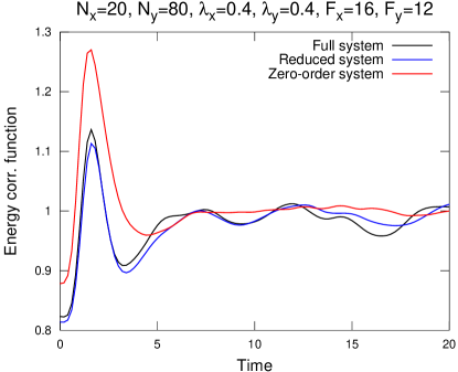
Figure 4.10. Energy autocorrelation functions, $\lambda_{x}=\lambda_{y}=0.4$.

In addition, in Table 4.4 we show the $L_{2}$-errors in energy autocorrelation functions (for the correlation time interval of 20 time units, as in Figures 4.9 and 4.10) between the full two-scale Lorenz model and the two reduced models. Observe that, generally, the reduced system with the linear correction term in (3.10) produces more precise results than its poor man’s version without the correction term.

$\lambda_{x,y}=0.3$, $F_{y}=8$ $\lambda_{x,y}=0.3$, $F_{y}=12$ Av. Z.O. $F_{x}=6$ $8.911\cdot 10^{-3}$ $2.027\cdot 10^{-2}$ $F_{x}=16$ $6.885\cdot 10^{-3}$ $1.434\cdot 10^{-2}$ Av. Z.O. $F_{x}=6$ $6.783\cdot 10^{-3}$ $2.131\cdot 10^{-2}$ $F_{x}=16$ $4.154\cdot 10^{-3}$ $1.455\cdot 10^{-2}$

$\lambda_{x,y}=0.4$, $F_{y}=8$ $\lambda_{x,y}=0.4$, $F_{y}=12$ Av. Z.O. $F_{x}=6$ $2.66\cdot 10^{-2}$ $0.2779$ $F_{x}=16$ $9.746\cdot 10^{-3}$ $2.284\cdot 10^{-2}$ Av. Z.O. $F_{x}=6$ $3.499\cdot 10^{-2}$ $0.3125$ $F_{x}=16$ $5.49\cdot 10^{-3}$ $2.414\cdot 10^{-2}$

Table 4.4. $L_{2}$-errors between the energy autocorrelation functions of the slow variables of the full two-scale Lorenz model and the two reduced models. Notations: “Red.” stands for “Reduced” (that is, (3.10)), and “Z.O.” stands for “Zero-order”, the poor man’s version of (3.10).

5. Summary

In this work we develop a simple method of constructing the closed reduced model for slow variables of a multiscale model with linear coupling, which requires only a single computation of the mean state and the time autocorrelation function for the fast dynamics with a fixed state of the slow variables, which is located in the region where the slow dynamics evolve (here, the mean state of the slow dynamics is used). The method is based on the first-order Taylor expansion of the averaged coupling term with respect to the slow variables, which is computed using the linear fluctuation-dissipation theorem. We demonstrate through the computations with the appropriately rescaled two-scale Lorenz 96 model [4] that, with simple linear coupling in both slow and fast variables, the developed reduced model produces quite comparable statistics to what is exhibited by the complete two-scale Lorenz model. Below we outline the main advantages of the new method:

• The reduced model is simple. It requires only the mean state, covariance and the time autocorrelation function for the fast variables, computed for a single fixed state of the slow variables. Since only the statistics of the time series of the fast dynamics are needed, the structure of the right-hand side of the equations for the fast variables need not be known explicitly – this part of dynamics can be provided as a “black box”. Also, the structure of the nonlinear $\boldsymbol{x}$-dependent part of the right-hand side of the equations for the slow variables need not be known to construct the approximation, and existing computational routines can be used for it. The only correction in the forward time-stepping routine is the linear correction term.

• The reduced model is a priori. It lacks parameters which have to be adjusted a posteriori to “fit” the statistical properties of the full multiscale dynamics. In fact, statistical properties of the full multiscale dynamics need not be known to construct the reduced model (although certain statistics of the fast variables with an appropriate fixed slow state need to be computed).

• The reduced model is parsimonious. It requires only a simple linear correction to achieve consistently better performance than that of a corresponding zero-order model.

• The reduced model is practical. It can be implemented even when the statistics for the slow variables of the complete multiscale dynamics cannot be obtained due to its computational complexity (although a rough estimate of the mean state, or a nearby state is needed), which makes the approach potentially suitable for comprehensive global circulation models in geophysics. Additionally, existing zero-order models (such as the T21 barotropic model [7, 14, 30]) can be retrofitted with the linear correction term.

In the future work, the author intends to collaborate with geophysicists to create more realistic reduced models for geophysical dynamics, including retrofitting existing closed models for slow dynamics with the linear correction term.

References

- [1] R. Abramov. Short-time linear response with reduced-rank tangent map. Chin. Ann. Math., 30B(5):447–462, 2009.
- [2] R. Abramov. Approximate linear response for slow variables of deterministic or stochastic dynamics with time scale separation. J. Comput. Phys., 229(20):7739–7746, 2010.
- [3] R. Abramov. Improved linear response for stochastically driven systems. Front. Math. China, 2011. submitted.
- [4] R. Abramov. Suppression of chaos at slow variables by rapidly mixing fast dynamics through linear energy-preserving coupling. Comm. Math. Sci., 2011. submitted.
- [5] R. Abramov and A.J. Majda. Blended response algorithms for linear fluctuation-dissipation for complex nonlinear dynamical systems. Nonlinearity, 20:2793–2821, 2007.
- [6] R. Abramov and A.J. Majda. New approximations and tests of linear fluctuation-response for chaotic nonlinear forced-dissipative dynamical systems. J. Nonlin. Sci., 18(3):303–341, 2008.
- [7] R. Abramov and A.J. Majda. New algorithms for low frequency climate response. J. Atmos. Sci., 66:286–309, 2009.
- [8] R. Abramov and A.J. Majda. Low frequency climate response of quasigeostrophic wind-driven ocean circulation. J. Phys. Oceanogr., 2011. submitted.
- [9] R. Buizza, M. Miller, and T. Palmer. Stochastic representation of model uncertainty in the ECMWF Ensemble Prediction System. Q. J. R. Meteor. Soc., 125:2887–2908, 1999.
- [10] D. Crommelin and E. Vanden-Eijnden. Subgrid scale parameterization with conditional Markov chains. J. Atmos. Sci., 65:2661–2675, 2008.
- [11] W. E and X. Li. Some recent progress in multiscale modeling. In S. Attinger and P. Koumoutsakos, editors, Multiscale Modelling and Simulation, volume 39 of LNCSE. Springer, 2004.
- [12] J. Eckmann and D. Ruelle. Ergodic theory of chaos and strange attractors. Rev. Mod. Phys., 57(3):617–656, 1985.
- [13] I. Fatkullin and E. Vanden-Eijnden. A computational strategy for multiscale systems with applications to Lorenz 96 model. J. Comp. Phys., 200:605–638, 2004.
- [14] C. Franzke. Dynamics of low-frequency variability: Barotropic mode. J. Atmos. Sci., 59:2909–2897, 2002.
- [15] C. Franzke, A.J. Majda, and E. Vanden-Eijnden. Low-order stochastic model reduction for a realistic barotropic model climate. J. Atmos. Sci., 62:1722–1745, 2005.
- [16] K. Hasselmann. Stochastic climate models, part I, theory. Tellus, 28:473–485, 1976.
- [17] E. Lorenz. Predictability: A problem partly solved. In Proceedings of the Seminar on Predictability, Shinfield Park, Reading, England, 1996. ECMWF.
- [18] E. Lorenz and K. Emanuel. Optimal sites for supplementary weather observations. J. Atmos. Sci., 55:399–414, 1998.
- [19] A.J. Majda, R. Abramov, and M. Grote. Information Theory and Stochastics for Multiscale Nonlinear Systems, volume 25 of CRM Monograph Series of Centre de Recherches Mathématiques, Université de Montréal. American Mathematical Society, 2005. ISBN 0-8218-3843-1.
- [20] A.J. Majda, I. Timofeyev, and E. Vanden-Eijnden. Models for stochastic climate prediction. Proc. Natl. Acad. Sci., 96:14687–14691, 1999.
- [21] A.J. Majda, I. Timofeyev, and E. Vanden-Eijnden. A mathematical framework for stochastic climate models. Comm. Pure Appl. Math., 54:891–974, 2001.
- [22] A.J. Majda, I. Timofeyev, and E. Vanden-Eijnden. A priori tests of a stochastic mode reduction strategy. Physica D, 170:206–252, 2002.
- [23] A.J. Majda, I. Timofeyev, and E. Vanden-Eijnden. Systematic strategies for stochastic mode reduction in climate. J. Atmos. Sci., 60:1705–1722, 2003.
- [24] T. Palmer. A nonlinear dynamical perspective on model error: A proposal for nonlocal stochastic-dynamic parameterization in weather and climate prediction models. Q. J. R. Meteor. Soc., 127:279–304, 2001.
- [25] G. Papanicolaou. Introduction to the asymptotic analysis of stochastic equations. In R. DiPrima, editor, Modern modeling of continuum phenomena, volume 16 of Lectures in Applied Mathematics. American Mathematical Society, 1977.
- [26] F. Risken. The Fokker-Planck Equation. Springer-Verlag, New York, second edition, 1988.
- [27] D. Ruelle. A measure associated with Axiom A attractors. Amer. J. Math., 98:619–654, 1976.
- [28] D. Ruelle. Differentiation of SRB states. Comm. Math. Phys., 187:227–241, 1997.
- [29] D. Ruelle. General linear response formula in statistical mechanics, and the fluctuation-dissipation theorem far from equilibrium. Phys. Lett. A, 245:220–224, 1998.
- [30] F. Selten. An efficient description of the dynamics of barotropic flow. J. Atmos. Sci., 52:915–936, 1995.
- [31] G. Uhlenbeck and L. Ornstein. On the theory of the Brownian motion. Phys. Rev., 36:823–841, 1930.
- [32] E. Vanden-Eijnden. Numerical techniques for multiscale dynamical systems with stochastic effects. Comm. Math. Sci., 1:385–391, 2003.
- [33] V. Volosov. Averaging in systems of ordinary differential equations. Russian Math. Surveys, 17:1–126, 1962.
- [34] D. Wilks. Effects of stochastic parameterizations in the Lorenz ’96 system. Q. J. R. Meteorol. Soc., 131:389–407, 2005.
- [35] L.-S. Young. What are SRB measures, and which dynamical systems have them? J. Stat. Phys., 108(5-6):733–754, 2002.