Observational consequences of the Standard Model Higgs inflation variants

Abstract

We consider the possibility to observationally differentiate the Standard Model (SM) Higgs driven inflation with non-minimal coupling to gravity from other variants of SM Higgs inflation based on the scalar field theories with non-canonical kinetic term such as Galileon-like kinetic term and kinetic term with non-minimal derivative coupling to the Einstein tensor.
In order to ensure consistent results, we study the SM Higgs inflation variants by using the same method, computing the full dynamics of the background and perturbations of the Higgs field during inflation at quantum level.
Assuming that all the SM Higgs inflation variants are consistent theories, we use the MCMC technique to derive constraints on the inflationnoary parameters and the Higgs boson mass from their fit to WMAP7+SN+BAO data set. We conclude that a combination of a Higgs mass measurement by the LHC and accurate determination by the PLANCK satellite of the spectral index of curvature perturbations and tensor-to-scalar ratio will enable to distinguish among these models. We also show that the consistency relations of the SM Higgs inflation variants are distinct enough to differentiate the models.

1 Introduction

There has been much interest recently in models of inflation in which the Standard Model (SM) Higgs boson non-minimally coupled to the Ricci scalar can give rise to inflation without the need for additional degrees of freedom to the SM [1, 2, 3, 4, 5]. This scenario is based on the observation that the problem of the very small value of the Higgs quadratic coupling required by the Cosmic Microwave Background (CMB) anisotropy data can be solved if the Higgs inflaton has a large non-minimally coupling with gravity [6]. The resultant Higgs inflaton effective potential in the inflationary domain is effectively flat and can result in successful inflation for values of non-minimally coupling constant $\zeta\sim 10^{4}$ ($\zeta$-inflation), allowing for cosmological values for Higgs boson mass in a window in which the electroweak vacuum is stable and therefore sensitive to the field fluctuations during the early stages of the universe [7].
Limits of validity of $\zeta$-inflation have been recently debated by several authors. Specifically, Barbon & Espinosa (2009) argued that the large coupling of Higgs inflaton to the Ricci scalar makes this model invalid beyond the ultraviolet cutoff scale $\Lambda_{\zeta}\simeq M_{P}/\zeta$ (hereafter $M_{P}=2.4\times 10^{18}$ GeV is the reduced Planck mass) which is below the Higgs field expectation value at $\cal N$ e-foldings during inflation, $\phi\simeq\sqrt{N}M_{P}/\sqrt{\zeta}$. As consequence, at the ultraviolet cutoff scale $\Lambda_{\zeta}$ at least one of the cross-sections of different scattering processes hits the unitarity bound [9]. The fact that the quantum corrections due to the strong coupling to gravity makes the perturbative analysis to break down at energy scales above $\Lambda_{\zeta}$ was interpreted as a signature of a new physics, implying higher dimensional operators at energies above $\Lambda_{\zeta}$. Few authors addressed the issue of $\zeta$-inflation naturalness with respect to perturbativity and unitarity violation in Jordan and Einstein frames [10, 11, 12, 13]. They show that the apparent breakdown of the theory in the Jordan frame does not imply new physics, but a failure of the perturbation theory in the Jordan frame as a calculation method. These works demonstrate that, for inflation based on a single scalar field with large non-minimal coupling, the quantum corrections at high energy scales are small, making the perturbative analysis valid and consequently there is no a breakdown of unitarity at the energy scale $\Lambda_{\zeta}$.
Recent works [14, 15, 16] revisit the issue of self-consistency of $\zeta$-inflation model emphasizing that the scale of unitarity violation depends on the size of the Higgs background field. They found the cutoff scale $\Lambda_{\zeta}$ higher than the relevant dynamical scales throughout the whole history of the universe, including the inflationary epoch and reheating, indicating that the theory does not violate unitarity at any time.
Although the above conclusion theoretically may allow to work within the regime of validity of the effective theory for inflationary calculations, other variants of Higgs inflation within the SM have been proposed. These models are based on scalar field theories with non-canonical kinetic term [17] and are motivated by some particle physics models of inflation such us the Dirac-Born-Infed inflation [18, 19].

A model with non-minimal derivative couplings was proposed in [20, 21, 22] in context of inflationary cosmology, and recently, the inflation driven by a scalar field with a Higgs potential and non-minimal kinetic couplings to itself and to the curvature was proposed in [23, 24]. In the new model of Higgs inflation (E-inflation) an enhanced kinetic term in the Lagrangian propagating no more degrees of freedom than the minimally coupled scalar field in General Relativity (GR) is obtained by considering non-minimal derivative coupling of the SM Higgs boson to the Einstein tensor [25]. The power counting analysis indicates that the scale at which the unitarity bound is violated in this model is $\Lambda(H)\simeq(2H^{2}\kappa)^{1/3}$, where $H$ is the Hubble expansion during inflation. Requiring the unitarity constraint $H\ll\Lambda$ to be satisfied, it is shown that the non-minimal derivative coupling allows a Higgs boson self-coupling value $\lambda$ within the limits expected from the collider experiments while the cosmological perturbations in this model are consistent with present cosmological data [26, 27].

The Galileon models of inflation (G-inflation) are constructed by introducing a scalar field with a self-interaction whose Lagrangian is invariant under Galileon symmetry $\partial_{\mu}\phi\rightarrow\partial_{\mu}\phi+b_{\mu}$, which maintains the equation of motion of the scalar field as a second-order differential equation, preventing the theory from exhibiting new degrees of freedom and avoiding ghost or instability problems [28, 29, 30]. Recently, an inflation model in which inflation is driven by the SM Higgs scalar field with a Galileon-like kinetic term has been proposed [31]. The dynamics of background and perturbations of G-inflaton show new features brought by the modified kinetic term in the Lagrangian, when compared with the standard slow-roll inflation, such as: violation of the standard consistency relation [31, 32], violation of the Null Energy Condition [33], generation of isocurvature perturbations and large primordial non-Gaussianity [34, 35, 36, 37].

In this paper we analyze to possibility to distinguish among the SM Higgs inflation variants by using the existing cosmological and astrophysical measurements. We will adopt a similar philosophy as in [38], considering that the SM Higgs inflation variants are consistent theories and therefore should be subject to rigorous tests against experimental data.
Cosmological constraints on the SM Higgs driven $\zeta$-inflation have been discussed by a number of authors [2, 3, 4]. These constraints are based on mapping between the Renormalization Group (RG) flow equations and the spectral index of the curvature perturbations obtained by the WMAP team, parametrized in terms of the number of ${\it e}$-foldings till the end of inflation. In a recent paper [39] we studied the implications of the full dynamics of background and perturbations of the Higgs field during $\zeta$-inflation at quantum level and derive constaints on the inflationary parameters and the Higgs boson mass from the analysis of WMAP 7-year CMB measurements complemented with astrophysical distance measurements [45, 46].
Our goal in this paper is to refine the computation for $\zeta$-inflation by considering in the analysis the improved RG flow equations, accounting at the same time for the possible uncertainties in the theoretical determination of the reheating temperature. We also make a similar analysis for G-inflation and E-inflation models and derive constraints on the inflationary parameters and Higgs boson mass from their fit to the same data set, ensuring in this way that the differences in the predictions of the observables are due to the differences in the underlying theories of the SM Higgs inflation and therefore can be used to distinguish among them.

The paper is organized as follows. In Section 2 we introduce the there models of the SM Higgs inflation that we consider: $\zeta$-inflation [1], G-inflation [31] and E-inflation [25, 26]. In Section 3 we compute the RG improved Higgs field potential and in Section 4 we present our main results. In Section 5 we draw our conclusions.
Throughout the paper we consider an homogeneous and isotropic flat background described by the Friedmann-Robertson-Walker (FRW) metric:

$${\rm d}s^{2}=g_{\mu,\nu}\,{\rm d}x_{\mu}\,{\rm d}x^{\nu}=-{\rm d}t^{2}+a^{2}(t){\rm d}x^{2}\,,$$ (1.1)

where $a$ is the cosmological scale factor, $\kappa^{2}\equiv 8\pi M_{pl}^{-2}$ (where $M_{pl}\simeq 1.22\times 10^{19}$ GeV is the Planck mass), overdots denotes the time derivatives and ${}_{,X}\equiv\partial/\partial{X}$.
We also remind that the canonical tree-level action describing the SM Higgs inflation is given by:

$$S_{0}=\int{{\rm d}^{4}\,x}\sqrt{-g}\,\left[\frac{1}{2\kappa^{2}}{\bf R}+{\cal L}_{SM}\right]\,,$$ (1.2)

where ${\bf R}$ is the Ricci scalar and ${\cal L}_{SM}$ is the tree-level SM Higgs Lagrangian:

$${\cal L}_{SM}=g^{\mu\nu}{\cal D}_{\mu}{\cal H}^{\dagger}{\cal D}_{\nu}{\cal H}-\lambda\left({\cal H}^{\dagger}{\cal H}-v^{2}\right)^{2}\,.$$ (1.3)

In the above expression ${\cal H}$ is the Higgs boson doublet, ${\cal D}_{\mu}$ is the covariant derivative with respect to $SU(2)\times SU(1)$ and $v$ is the vacuum expectation value (vev) of the Higgs broken phase of the SM. Rotating the Higgs doublet such that ${\cal H}^{T}=(1/\sqrt{2})(0,v+\phi)$ and assuming that $\phi$ is much greather than vev during inflation we have:

$${\cal L}_{SM}=P(\phi,X)=X-V(\phi)\,,\hskip 28.45274ptX=-\frac{1}{2}g^{\mu\nu}\partial_{\mu}\partial_{\nu}\phi\,,\hskip 28.45274ptV(\phi)=\frac{\lambda}{4}\phi^{4}\,,$$ (1.4)

where $\lambda$ is the tree-level Higgs self coupling and $V(\phi)$ is the corresponding Higgs potential.

2 Models: background equations and cosmological perturbations

In this section we derive the background equations of motion of the scalar field and present the power spectra of scalar and tensor perturbations derived in the framework of linear cosmological perturbation theory for the SM Higgs inflation models that we consider. A review of chaotic inflation formalism in modified gravitational theories can be found in [40].

2.1 Higgs driven $\zeta$-inflation

The general action for these models in the Jordan frame is given by [41, 40]:

$$S_{J}\equiv\int d^{4}x\sqrt{-g}\left[U(\phi){\bf R}-\frac{1}{2}G(\phi)(\nabla\phi)^{2}-V(\phi)\right]\,,$$ (2.1)

where $U(\phi)$ is a general coefficient of the Ricci scalar, R, giving rise to the non-minimal coupling, $G(\phi)$ is the general coefficient of kinetic energy and $V(\phi)$ is the general potential.
The generalized $U(\phi)$R gravity theory in Equation (2.1) includes diverse cases of coupling. For generally coupled scalar field $U=(\gamma+\kappa^{2}\zeta\phi^{2})$, $G(\phi)=1$ and $\gamma$ and $\zeta$ are constants. The non-minimally coupled scalar field is the case with $\gamma=1$ while the conformal coupled scalar field is the case with $\gamma=1$ and $\zeta=1/6$. The conformal transformation for the action given in Equation (2.1) can be achieved by defining the Einstein frame line element:

$${\rm d}{\hat{s}}^{2}=\Omega\left(-{\rm d}{\hat{t}}^{2}+\hat{a}^{2}({\hat{t}}){\rm d}x^{2}\right)\,,\hskip 14.22636pt\Omega=2\kappa^{2}U(\phi)\,,\hskip 14.22636ptU(\phi)=(1+\kappa^{2}\zeta\phi^{2})\,,$$ (2.2)

where the quantities in the Einstein frame are marked by caret. From the above equations we get:

$${\rm d}\hat{a}=\sqrt{\Omega}\,{\rm d}a\,,\hskip 28.45274pt{\rm d}\hat{t}=\sqrt{\Omega}\,{\rm d}t\,,$$ (2.3)

and scalar potential $\hat{V}(\hat{\phi})$ in the Einstein frame is given by:

$$\hat{V}(\hat{\phi})=\frac{1}{4\kappa^{4}}\frac{V(\phi)}{U^{2}(\phi)}\,.$$ (2.4)

The non-minimal coupling to the gravitational field introduces a modification of the Higgs field propagator by a suppresion factor $s(\hat{\phi})$ defined as [4, 49]:

$$s(\hat{\phi})^{-2}=\left(\frac{{\rm d}\hat{\phi}}{{\rm d}\phi}\right)^{2}=\frac{1}{2\kappa^{2}}\frac{G(\phi)U(\phi)+3U^{2}(\phi)_{,\phi}}{U^{2}(\phi)}\,,$$ (2.5)

that made the kinetic energy in the Einstein frame canonical with respect to the the new scalar field ${\hat{\phi}}$.
Background equations. The Friedmann equation in the Einstein frame reads as [42, 44]:

$$\hat{H}^{2}=\frac{\kappa^{2}}{3}\left[\left(\frac{{\rm d}\hat{\phi}}{{\rm d}\hat{t}}\right)^{2}+\hat{V}(\hat{\phi})\right]\,,\\$$ (2.6)

where:

$$\hat{H}\equiv\frac{1}{\hat{a}}\frac{{\rm d}\hat{a}}{{\rm d}\hat{t}} = \frac{1}{\sqrt{\Omega}}\left[H+\frac{1}{2\Omega}\frac{{\rm d}\Omega}{{\rm d}t}\right]\,,$$ (2.7)

$$\frac{{\rm d}\hat{\phi}}{{\rm d}\hat{t}} = \left(\frac{{\rm d}\hat{\phi}}{{\rm d}\phi}\right)\left(\frac{{\rm d}t}{{\rm d}\hat{t}}\right)\dot{\phi}$$ (2.8)

Equations (2.7) and (2.8) are enough to compute the background field evolution in the Einstein frame once the field equations in the Jordan frame are known.
The Jordan-frame field equations from action (2.1) are obtained as [43]:

$$H^{2}=\frac{\kappa^{2}}{3\,(1+\kappa^{2}\zeta\phi^{2})}\left[V(\phi)+\frac{1}{2}\dot{\phi}^{2}-6\,\zeta H\phi\dot{\phi}\right]\,,$$ (2.9)

$$\ddot{\phi}+3H\dot{\phi}+\left(\frac{\kappa^{2}\zeta\phi^{2}(1+6\zeta)}{1+\kappa^{2}\zeta\phi^{2}(1+6\zeta)}\right)\frac{\dot{\phi}^{2}}{\phi}=\frac{\kappa^{2}\zeta\phi V(\phi)-(1+\kappa^{2}\zeta\phi^{2})V_{,\,\phi}(\phi)}{1+\kappa^{2}\zeta\phi^{2}(1+6\zeta)}\,,$$ (2.10)

that in the slow-roll approximation ( $|\dot{\phi}/\phi|\ll H$ and $|\dot{\phi}^{2}|\ll V(\phi)$ ) can be written as:

$$H^{2} \simeq \frac{\kappa^{2}}{3(1+\kappa^{2}\zeta\phi^{2})}V(\phi)\,,$$ (2.11)

$$3H\dot{\phi} \simeq \frac{\kappa^{2}\zeta\phi V(\phi)-(1+\kappa^{2}\zeta\phi^{2})V_{,\,\phi}(\phi)}{1+\kappa^{2}\zeta\phi^{2}(1+6\zeta)}\,.$$ (2.12)

Cosmological perturbations. Introducing the following quantities

$$\hat{Q_{S}}=\left(\frac{{\rm d}\hat{\phi}/{\rm d}\hat{t}}{\hat{H}}\right)^{2}\,,\hskip 28.45274pt\hat{\epsilon}=-\frac{{\dot{\hat{H}}}}{\hat{H}^{2}}\,,\hskip 28.45274pt\hat{\delta}_{S}=\frac{{\dot{\hat{Q}}}_{S}}{2\hat{H}\hat{Q}_{S}}\,,$$

$${\hat{\gamma}_{S}}=\frac{(1+{\hat{\delta}}_{S})(2+{\hat{\delta}}_{S})+{\hat{\epsilon}})}{(1+{\hat{\epsilon}})^{2}}\,,\hskip 28.45274pt{\hat{\nu}}_{S}=\sqrt{{\hat{\gamma}}_{S}+1/4}\,,$$ (2.13)

the power spectrum of the curvature perturbations in the Einstein frame is given by [43, 44]:

$${\cal P}_{\cal R}=\frac{1}{{\hat{Q}}_{S}}\left(\frac{{\hat{H}}}{2\pi}\right)^{2}\left(\frac{1}{{\hat{a}}{\hat{H}}|\tau|}\right)^{2}\left(\frac{\Gamma({\hat{\gamma}}_{S})}{\Gamma(3/2)}\right)^{2}\left(\frac{k|\tau|}{2}\right)^{3-2{\hat{\nu}}_{S}}\,.$$ (2.14)

where $\tau=-1/[(1+{\hat{\epsilon}}{\hat{a}}{\hat{H}}]$ is the conformal time.
The spectral index of the curvature perturbations obtained as usual as $n_{S}\equiv 1+d\,{\rm ln}{\cal P}_{S}(k)/d\,{\rm ln}k$ is:

$$n_{S}-1=3-2{\hat{\nu}}_{S}=3-\sqrt{4{\hat{\gamma}}_{S}+1}\,.$$ (2.15)

The power spectrum of the tensor perturbations in the Einstein frame is obtained from Equation (2.14) making the following replacements:

$${\hat{Q}}_{S}\rightarrow{\hat{Q}}_{T}=1\,,\hskip 14.22636pt{\hat{\gamma}}_{S}\rightarrow{\hat{\gamma}}_{T}=\frac{(1+{\hat{\delta}}_{T})(2+{\hat{\delta}}_{T})+{\hat{\epsilon}})}{(1+{\hat{\epsilon}})^{2}}\,,\hskip 14.22636pt\hat{\delta}_{S}\rightarrow{\hat{\delta}_{T}}=\frac{{\dot{\hat{Q}}}_{T}}{2\hat{H}\hat{Q}_{T}}=0\,.$$ (2.16)

The spectral index of the tensor perturbations $n_{T}$ and the tensor-to-scalar ratio $R$ are then given by:

$$n_{T}=3-\sqrt{4{\hat{\gamma}}_{T}+1}\,\hskip 28.45274ptR=8\frac{{\hat{Q}}_{S}}{{\hat{Q}}_{T}}\left(\frac{\Gamma({\hat{\gamma}}_{T})}{\Gamma({\hat{\gamma}}_{S})}\right)^{2}\,.$$ (2.17)

2.2 Higgs driven G-inflation

In this section we consider that inflation is driven by the SM Higgs potential with a kinetic term modified by a function $G(\phi,X)$ such that the standard part of the Lagrangian given in Equation (1.4) remains much larger than the Galileon interaction term, taking the form [31]:

$${\cal L}_{G}(\phi,X)=P(\phi,X)-G(\phi,X)\Box\phi\,,\hskip 8.5359pt{\rm where}\hskip 8.5359pt|P(X,\phi)|\simeq V(\phi)\gg|G(X,\phi)\Box\phi|\,.$$ (2.18)

Background equations. The energy density and pressure of the homogeneous and isotropic background field described by the FRW metric are [32, 37]:

$$\rho = 2P_{,X}X-P+6G_{,X}H\dot{\phi}X-G_{,\phi}X\,,$$ (2.19)

$$p = P-(G_{,\phi}+G_{,X}\ddot{\phi})X\,,$$ (2.20)

where $H=\dot{a}/a$ is the Hubble parameter. The gravitational field equations are then given by:

$$3\kappa^{2}H^{2}=\rho\,,\hskip 28.45274pt-\kappa^{2}\left(2H^{2}+2\dot{H}\right)=p\,,$$ (2.21)

and the scalar field equation of motion reads as:

$$P_{,X}(\ddot{\phi}+3H\dot{\phi})+2P_{XX}X\ddot{\phi}+2P_{,X\phi}X-P_{,\phi}-2G_{,X\phi}X(\ddot{\phi}-3H\dot{\phi})$$ (2.22)

$$+6G_{,X}[(HX)+3H^{2}X]-2G_{,\phi\phi}X+6G_{,XX}HX\dot{X}=0\,.$$

Since we are interesting in fluctuations generated during inflation, we assume a background for which the quantities $|\ddot{\phi}/(H\dot{\phi})|$ and $|G_{,\phi}\dot{\phi}/(GH)|$ are much smaller than unity. Under these assumptions, the first slow-roll parameter can be written as [34]:

$$\epsilon\equiv-\frac{\dot{H}}{H^{2}}=\frac{XP_{,X}+3G_{,X}H\dot{\phi}X}{\kappa^{2}H^{2}}\ll 1\,,$$ (2.23)

and the sound speed of scalar perturbations is given by:

$$c^{2}_{s}\equiv\frac{\partial_{X}\,p}{\partial_{X}\,\rho}=\frac{\cal F}{\cal G}\,,$$ (2.24)

where:

$${\cal F} = P_{,X}+4\dot{\phi}H\,G_{,X}\,,$$ (2.25)

$${\cal G} = P_{,X}+2XP_{,XX}+6H\dot{\phi}(G_{,X}+XG_{,XX})\,.$$ (2.26)

Cosmological perturbations. The CMB temperature anisotropy directly relates to the statistical properties of the primordial curvature perturbations ${\cal R}$ on large scales:

$${\cal R}=-\frac{H}{\dot{\phi}}Q\,,$$ (2.27)

where $\phi$ is the background value of the field and $Q$ is the perturbation in the unitary gauge, $\phi({\bf x},t)=\phi(t)$, with $\delta\phi=0$. The second order action in this gauge at leading order in the slow-roll approximation reads as:

$$S_{2}=\frac{1}{2\pi^{2}}\int{\rm d}{\tau}{\rm d}^{3}x\frac{a^{3}}{2c^{2}_{s}}(P_{,X}+4{\dot{\phi}}HG_{\,X})\left[{\dot{Q}}^{2}-\frac{c^{2}_{s}}{a^{2}}\partial^{i}Q\partial_{i}Q\right]\,,$$ (2.28)

where $\tau$ is the conformal time. One should note that in the case of G-inflation the unitary gauge does not coincide with the comoving gauge [31] as in the case of K-inflation for which the scalar field Lagrangian is $L_{\phi}=P(X,\phi)$ [47]. Consequently, there are two independent solutions of the perturbation equation resulting from the second order action (2.28). Introducing the following parameters

$$\nu\equiv\frac{G_{,X}{\dot{\phi}}X}{\kappa^{2}H}\,,\hskip 28.45274pt{\tilde{\epsilon}}\equiv\epsilon+\nu\,,$$ (2.29)

the power spectra for $Q$ and ${\cal R}$ are obtained as [34]:

$$P_{Q}=\frac{X}{4\pi^{2}M^{2}_{pl}c_{s}\tilde{\epsilon}}\,,\hskip 42.67912ptP_{\cal R}=\frac{1}{8\pi^{2}M^{2}_{pl}}\frac{H^{2}}{c_{s}\tilde{\epsilon}}\,,$$ (2.30)

which are evaluated at the time of sound horizon exit $c_{s}k=aH$. Defining the additional slow-roll parameters:

$$\tilde{\eta}\equiv\frac{\dot{\tilde{\epsilon}}}{\tilde{\epsilon}H}\,,\hskip 28.45274pts\equiv\frac{\dot{c_{s}}}{c_{s}H}\,,$$ (2.31)

the spectral index of the curvature perturbations is obtained as:

$$n_{s}-1=\frac{{\rm d}P_{\cal R}(k)}{{\rm d\,ln}k}=-2\epsilon-\tilde{\eta}-s\,.$$ (2.32)

The power spectrum and the spectral index of tensor perturbations are given as usual in the form:

$$P_{T}=\frac{2H^{2}}{\pi^{2}M^{2}_{pl}}\,,\hskip 28.45274ptn_{T}=-2\epsilon\,.$$ (2.33)

Thus, the tensor-to-scalar ratio $R$ is:

$$R\equiv\frac{P_{T}}{P_{\cal R}}=-8c_{s}(n_{T}-2\nu)\,,$$ (2.34)

that highlights the difference between G-inflation model and K-inflation model for which $R=-8c_{s}n_{T}$.

Hereafter we will consider Higgs potential driven G-inflation corresponding to the following setup [32]:

$$G(\phi,X)=-g(\phi)X\,,\hskip 42.67912ptg(\phi)=\frac{\phi}{w^{4}}\,,$$ (2.35)

where $w$ is a mass parameter assumed to be positive. Under the slow-roll conditions, the energy density is dominated by the potential energy and the standard part of the kinetic term in the Lagrangian given in equation (2.18) takes the form $|P(\phi,X)|\simeq V(\phi)$. The speed of sound corresponding to this setup is $c^{2}_{s}\simeq 2/3$ and the Friedmann equation and the equation of motion of the scalar field read as:

$$H^{2}\simeq\frac{\kappa^{2}}{12}\lambda\phi^{2}\,,\hskip 42.67912pt{\dot{\phi}^{3}}\simeq-\frac{2}{3}\frac{\kappa^{2}H}{g(\phi)}\epsilon\,.$$ (2.36)

2.3 Higgs driven E-inflation

In the recently proposed SM Higgs inflation model (E-inflation) with non-minimal derivative coupling to gravity [25], the tree-level SM Higgs Lagrangian takes the form:

$${\cal L}_{E}(X,\phi)=-\frac{1}{2}\left(g^{\mu\nu}-w^{2}G^{\mu\nu}\right)\partial_{\mu}\phi\partial_{\nu}\phi-V(\phi)\,,\hskip 14.22636ptG^{\mu\nu}=R^{\mu\nu}-\frac{\bf R}{2}g^{\mu\nu}\,,$$ (2.37)

where ${\bf R}$ is the Ricci scalar, $G^{\mu\nu}$ is the Einstein tensor, $w$ is a mass parameter and $V(\phi)$ is the Higgs potential.
Background equations. The Friedmann equation and the field equation of motion are given by:

$$H^{2}=\frac{\kappa^{2}}{6}\left[\dot{\phi}^{2}(1+9H^{2}w^{2})+\frac{\lambda}{2}\phi^{4}\right]\,,\hskip 14.22636pt\partial_{t}\left[a^{3}\dot{\phi}(1+3H^{2}w^{2})\right]=-a^{3}\lambda\phi^{3}\,.$$ (2.38)

Asking the solutions to obey the following constraints:

$$\epsilon\equiv-\frac{\dot{H}}{H^{2}}\ll 1\,,\hskip 14.22636pt9H^{2}w^{2}\dot{\phi}^{2}\ll\frac{\lambda}{2}\phi^{4}\,,\hskip 14.22636ptH\gg\frac{1}{3w}\,,\hskip 14.22636pt|\ddot{\phi}|\ll 3H|\dot{\phi}|\,,$$ (2.39)

Equations (2.38) can be written as:

$$H^{2}\simeq\frac{k^{2}}{12}\lambda\phi^{4}\,,\hskip 42.67912pt\dot{\phi}\simeq-\frac{4}{3Hw^{2}\kappa^{2}\phi}\,.$$ (2.40)

Cosmological perturbations. The power spectrum of the curvature perturbations evaluated at the time of sound horizon exit $c_{s}k=aH$ is obtained as solution of the perturbation equation resulting from the canonically normalized second order action [26]:

$${P}_{\cal R}=\frac{\kappa^{2}H^{2}}{4\pi^{2}}\frac{1}{12w^{2}\kappa^{2}\dot{\phi}^{2}}\left(1+\frac{19}{2}w^{2}\kappa^{2}\dot{\phi^{2}}\right)\,,$$ (2.41)

where the sound speed of the curvature perturbations is

$$0<c^{2}_{s}=\frac{3-13w^{2}\kappa^{2}{\dot{\phi}}^{2}}{3+18w^{2}\kappa^{2}{\dot{\phi}}^{2}}<1\,.$$ (2.42)

Introducing the first two slow-roll parameters:

$$\epsilon \equiv -\frac{\dot{H}}{H^{2}}=\frac{3}{2}\kappa^{2}w^{2}\dot{\phi}^{2}\hskip 14.22636pt\,,$$ (2.43)

$$\eta \equiv -\frac{\ddot{\phi}}{H\dot{\phi}}=-\frac{9}{4}\kappa^{2}w^{2}\dot{\phi}^{2}=-\frac{3}{2}\epsilon\,,$$ (2.44)

to leading order in slow-roll approximation ${P}_{\cal R}$ can then be written as:

$${P}_{\cal R}=\frac{\kappa^{2}H^{2}}{4\pi^{2}}\frac{1}{8\epsilon}\,,$$ (2.45)

and the spectral index of the curvature perturbations is

$$n_{S}-1=\frac{{\rm d\,ln}{\cal P}_{\cal R}}{{\rm d\,ln}k}=2\frac{{\rm d\,ln}H}{{\rm d\,ln}k}-\frac{{\rm d\,ln}\epsilon}{{\rm d\,ln}k}\,,$$ (2.46)

and by using Equations (2.43) and (2.44) can be written as:

$$n_{S}=1-2\epsilon-2\eta=1-5\epsilon\,.$$ (2.47)

The power spectrum of the tensor perturbations is obtained as:

$$P_{T}=\frac{\kappa^{2}H^{2}}{4\pi^{2}\Omega^{2}c^{3}_{g}}\,,$$ (2.48)

where $\Omega$ and the sound speed of the gravitational waves $c_{g}$ are:

$$\Omega^{2}=1-\frac{1}{2}w^{2}\kappa^{2}\dot{\phi}^{2}\,,\hskip 14.22636ptc^{2}_{g}\simeq 1+w^{2}\kappa^{2}\dot{\phi}^{2}\,.$$ (2.49)

To the leading order in $w^{2}\kappa^{2}\dot{\phi}^{2}$ we have $\Omega\simeq 1$ and $c_{g}\simeq 1$. The spectral index of the tensor perturbations is

$$n_{T}=\frac{{\rm d\,ln}{P}_{T}}{{\rm d\,ln}k}=-2\epsilon\,,$$ (2.50)

and the tensor-to-scalar ratio $R$ is given by:

$$R=\frac{{P}_{T}}{{P}_{\cal R}}=12w^{2}\kappa^{2}\dot{\phi}^{2}=8\epsilon\,.$$ (2.51)

3 Quantum corrections to the Higgs potential

The quantum corrections due to the interaction effects of the SM particles with Higgs boson through quantum loops modify Higgs scalar potential from classical expression in both Jordan and Einstein frames, taking the RG forms:

$$V(t)=\frac{\lambda(t)}{4}\phi(t)^{4}\,,\hskip 14.22636pt\hat{V}(t) = \frac{1}{16\kappa^{4}}\,\frac{\lambda(t)\phi^{4}(t)}{(1+\kappa^{2}\xi(t)\phi^{2}(t))^{2}}\,,\hskip 14.22636ptt={\rm ln}\left(\frac{\phi}{m_{Top}}\right)\,,$$ (3.1)

where the scaling variable $t$ normalizes the Higgs field and all the running couplings to the top quark mass scale $m_{Top}=171.3$ GeV [48]. We compute the various $t$-dependent running constants by integrating the RG $\beta$-functions as compiled in the Appendix. For each case, the $t$-dependent running constants are obtained as:

$$Y(t)=\int^{t}_{t=0}\frac{\beta_{Y}(t^{\prime})}{1+\gamma(t^{\prime})}\,{\rm d}t^{\prime}\,,\hskip 28.45274ptY=\{g,g^{\prime},g_{s},y_{t},\lambda,\zeta\}\,,$$ (3.2)

where $\gamma$ is the Higgs field anomalous dimension given by Equation (6.11) from Appendix.
At $t=0$, which corresponds to the top quark mass scale $m_{Top}$, the Higgs quadratic coupling $\lambda(0)$ and the top Yukawa coupling $y_{t}(0)$ are determined by the corresponding pole masses and the vacuum expectation value ${\it v}=246.22$ GeV as:

$$\lambda(0)=\frac{m^{2}_{H}}{2{\it v}^{2}}\left[1+2\Delta_{H}(m_{H})\right]\,,\hskip 42.67912pty_{t}(0)=\frac{\sqrt{2}m_{T}}{\it v}\left[1+\Delta_{T}(m_{T})\right]\,,$$ (3.3)

where $\Delta_{H}(m_{H})$ and $\Delta_{T}(m_{T})$ are the corrections to Higgs and top quark mass respectively, computed following the scheme from the Appendix of Espinosa et al.(2008). The initial values of the gauge coupling constants at $t=0$ are given by:

$$\frac{g^{2}(0)}{4\pi}=0.03344\,,\hskip 28.45274pt\frac{g^{\prime 2}(0)}{4\pi}=0.01027\,,\hskip 28.45274pt\frac{g^{2}_{s}(0)}{4\pi}=0.1071\,.$$ (3.4)

The couplings $g$ and $g^{\prime}$ are obtained by integrating RG flow equations from their values at $M_{Z}$, while $g_{s}$ is calculated numerically [49]. The value of non-minimally coupling constant $\zeta$ at the beginning of inflation is determined such that the calculated value of the amplitude of the curvature density perturbations agrees with the measured value [50].

4 RESULTS

4.1 The CMB Angular Power Spectra

We obtain the CMB temperature anisotropy and polarization power spectra by integrating the coupled Friedmann equation and equation of motion of the scalar field with respect to the conformal time corresponding to the SM Higgs inflation variants, as presented in the previous section. We take wavenumbers in the range $5\times 10^{-6}-5$ Mpc^-1 needed by CAMB Boltzmann code [51, 52] to numerically derive the CMB angular power spectra and a Hubble radius crossing scale $k_{*}=c_{s}k=0.002$Mpc^-1 and impose that the electroweak vacuum expectation value ${\it v}=$246.22 GeV is the true minimum of the Higgs potential at any energy scale ($\lambda(t)>$0).

The value of the Higgs scalar field at the beginning of inflation $\phi_{\cal N}$ determines the value of the scaling parameter $t={\rm ln}(\phi_{\cal N}/m_{Top})$ at this time.
For the case of $\zeta$-inflation the value of $\phi_{\cal N}$ relates to the quantum scale of inflation $\phi_{I}$ and to the duration of inflation expressed in units of e-folding number ${\cal N}$ through [2]:

$$\frac{\varphi^{2}_{*}}{\varphi_{I}} = e^{x}-1\,,\hskip 42.67912pt\varphi_{I}=\frac{64\pi^{2}M^{2}_{pl}}{\xi{\bf A_{I}}}\,,\hskip 42.67912ptx\equiv\frac{{\it N}{\bf A_{I}}}{48\pi^{2}}\,,$$ (4.1)

$${\bf A_{I}} = \frac{3}{8\lambda}\left(2g^{4}+(g^{2}+g^{\prime 2})^{2}-16y_{t}^{4}\right)-6\lambda\,,$$ (4.2)

where the inflationary anomalous scaling parameter ${\bf A_{I}}$ involves a special combination of quantum corrected coupling constants [6, 49].
The value of the field at the end of G-inflation is obtained from Equations (2.23) and (2.35) asking the solution to obey the condition $\epsilon=1$ at the end of G-inflation:

$$\phi_{end}=2^{3/4}\lambda^{-1/8}\kappa w^{1/2}\,.$$ (4.3)

The number of $e$-folds till the end of G-inflation is then given by:

$${\cal N}=\int^{\phi_{end}}_{\phi_{\cal N}}\frac{H}{{\dot{\phi}}}{\rm d}\phi=\frac{1}{16}\frac{\lambda^{1/2}}{\kappa^{2}w^{2}}\phi^{4}-\frac{1}{2}\,,$$ (4.4)

from which the value of the field evaluated ${\cal N}$ $e$-folds before the end of G-inflation is:

$$\phi_{\cal N}=(16{\cal N}+8)^{1/4}\lambda^{-1/8}\kappa w^{1/2}\,.$$ (4.5)

In a similar way, the value of the field at the end of E-inflation is obtained from Equations (2.40) and (2.43) by asking the solution to obey the condition $\epsilon=1$ at the end of E-inflation:

$$\phi^{6}_{end}=\frac{32}{w^{2}\kappa^{4}\lambda}\,,$$ (4.6)

From the evaluation of the number of e-foldings $\cal N$ during E-inflation:

$${\cal N}=\int^{\phi_{end}}_{\phi_{\cal N}}\frac{H}{\dot{\phi}}{\rm d}\phi=\frac{1}{96}\lambda w^{2}\kappa^{4}\left(\phi^{6}_{\cal N}-\phi^{6}_{end}\right)\,,$$ (4.7)

we obtain the value of the field at ${\cal N}$ e-folds before the end of E-inflation as:

$$\phi^{6}_{{\cal N}}=\frac{32}{w^{2}\kappa^{4}\lambda}\left(3{\cal N}+1\right)\,.$$ (4.8)

As the inflationary observables are evaluated at the epoch of horizon-crossing quantified by the number of e-foldings $\cal N$ before the end of the inflation at which our present Hubble scale equalled the Hubble scale during inflation, the uncertainties in the determination of $\cal N$ translates into theoretical errors in determination of the inflationary observables [53, 54]. Assuming that the ratio of the entropy per comoving interval today to that after reheating is negligible, the main uncertainty in the determination of $\cal N$ is given by the uncertainty in the determination of the reheating temperature $T_{r}$ after inflation.
The dynamics of the Higgs field during G-inflation show that the effect of Galileon-like interaction during reheating is very small and can be safely ignored because $g=\phi/w^{4}$ ($\phi\ll w)$ term is suppressed around the minimum of the potential [32].
In the case of E-inflation the constraint $wH\gg 1$ suppresses the canonically normalized field $\phi\sim(wH)^{-1}$ that becomes ineffective during reheating.
Recent studies of the reheating after $\zeta$-inflation estimates $T_{r}$ in the range [5, 55]:

$$3.4\times 10^{13}\,{\rm GeV}<T_{r}<\left(\frac{\lambda}{0.25})\right)^{1/4}\,1.1\times 10^{14}\,{\rm GeV}\,,$$ (4.9)

that translates into a negligible variation of the number of e-foldings with the Higgs mass ($\Delta N\sim 0.1$). The number of e-foldings at Hubble radius crossing scale $k_{*}$ is related to $T_{r}$ through [38]:

$${\cal N}={\rm ln}\left[\left(\frac{\rho_{R}}{\rho_{end}}\right)^{1/3}\left(\frac{g_{0}T^{3}_{0}}{g_{*}T^{3}_{r}}\right)^{1/3}H\lambda\right]\,,$$ (4.10)

where $g_{*}\simeq 106.5$ for the SM, $g_{0}\simeq 2$ and $T_{0}$ is the present value of the photon temperature. Taking the variation range of $T_{r}$ given in Equation (4.9) and ${\cal N}=$ 59 ${\it e}$-foldings at $k_{*}$, in the view of WMAP7+SN+BAO normalization at this scale, we obtain $57.8\leq{\cal N}\leq 60.2$ for the number of ${\it e}$-foldings at which $k_{*}$ exits the horizon.
Throughout, we will consider ${\cal N}$ varying in the above range for all SM Higgs inflation variants. In this way we conservatively included the same error $\Delta{\cal N}\simeq 1.17$ to account for possible uncertainties in the theoretical estimate of $T_{r}$.
For each wavenumber $k$ our code integrates the $\beta$-functions of the $t$-dependent running constant couplings in the observational inflationary window imposing that $k$ grows monotonically to the wavenumber $k_{*}$, eliminating at the same time those models violating the condition for inflation $\epsilon\equiv-{\dot{H}}/H^{2}\leq 1$.

4.2 Markov Chain Monte Carlo (MCMC) Analysis

We use MCMC technique to reconstruct the Higgs field potential and to derive constraints on the inflationary observables and the Higgs boson mass from the following datasets.
The WMAP 7-year data [45, 46] complemented with geometric probes from the Type Ia supernovae (SN) distance-redshift relation and the baryon acoustic oscillations (BAO). The SN distance-redshift relation has been studied in detail in the recent unified analysis of the published heterogeneous SN data sets - the Union Compilation08 [56, 57]. The BAO in the distribution of galaxies are extracted from Two Degree Field Galaxy Redshift Survey (2DFGRS) the Sloan Digital Sky Surveys Data Release 7 [58]. The CMB, SN and BAO data (WMAP7+SN+BAO) are combined by multiplying the likelihoods. We use these measurements especially because we are testing models deviating from the standard Friedmann expansion. These datasets properly enables us to account for any shift of the CMB angular diameter distance and of the expansion rate of the universe.
The likelihood probabilities are evaluated by using the public packages CosmoMC and CAMB [52, 51] modified to include the formalisms for the SM Higgs driven G-inflation and E-inflation as described in the previous sections.
The fiducial model is the $\Lambda$CDM standard cosmological model described by a set of parameters receiving uniform priors. For the case of G-inflation and E-inflation we used the following set of parameters:

$$\left\{\Omega_{b}h^{2}\,,\,\,\Omega_{c}h^{2}\,,\,\,\theta_{s}\,,\,\,\tau\,,\,\,m_{Higgs}\,,\,\,w\,,\,\,{\cal N}\right\}\,,$$

where: $\Omega_{b}h^{2}$ is the physical baryon density, $\Omega_{c}h^{2}$ is the physical dark matter density, $\theta_{s}$ is the ratio of the sound horizon distance to the angular diameter distance, $\tau$ is the reionization optical depth, $m_{Higgs}$ is the Higgs boson pole mass, $w$ is the mass parameter and $\cal N$ is the number of e-foldings at the Hubble radius crossing.
For the case of $\zeta$-inflation we used the same set of input parameters except for the mass parameter $w$. For this case we use as input the amplitude of the curvature perturbations $A^{2}_{S}\sim\lambda/\zeta^{2}$ that fix the value of the non-minimally coupling constant $\zeta$ at $k_{*}$ for a given value of the Higgs boson mass.
For each inflation model we run 64 Monte Carlo Markov chains, imposing for each case the Gelman & Rubin convergence criterion [59].

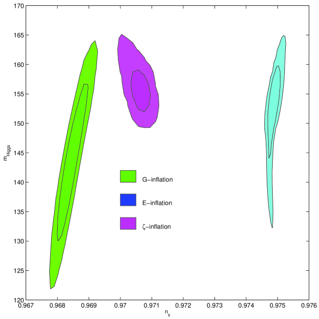
Figure 1: Two-dimensional marginalized joint probability distributions (68% and 95% CL) showing the dependence of the spectral index of the curvature perturbations $n_{S}$ on the Higgs inflaton mass $m_{Higgs}$ as obtained from the fit of the SM Higgs inflation variants with $m_{Top}$=171.3 GeV and ${\it v}$=246.22 GeV to the WMAP7+SN+BAO data set. All parameters are computed at the Hubble crossing scale $k_{*}$=0.002Mpc^-1.

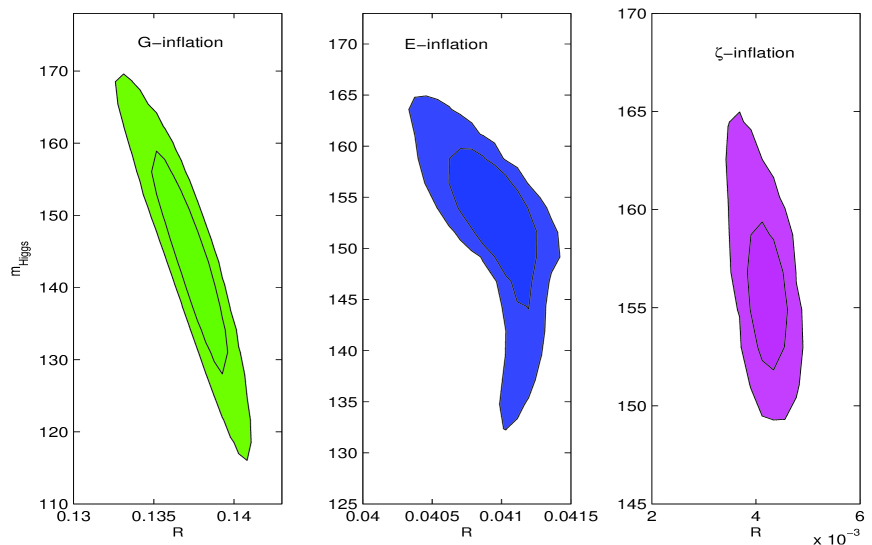
Figure 2: Two-dimensional marginalized joint probability distributions (68% and 95% CL) showing the dependence of the tensor-to-scalar ratio $R$ on the Higgs inflaton mass $m_{Higgs}$ as obtained from the fit of the SM Higgs inflation variants with $m_{Top}$=171.3 GeV and ${\it v}$=246.22 GeV to the WMAP7+SN+BAO data set. All parameters are computed at the Hubble crossing scale $k_{*}$=0.002Mpc^-1.

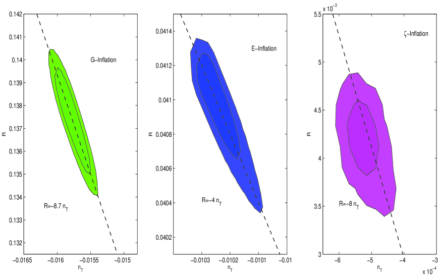
Figure 3: Two-dimensional marginalized joint probability distributions (68 % and 95% CL) showing the degeneracy between the spectral index of tensor perturbations $n_{T}$ and the tensor-to-scalar ratio $R$ obtained from the fit of SM Higgs inflation models with $m_{Top}$=171.3 GeV and ${\it v}$=246.22 GeV to the WMAP7+SN+BAO dataset. For each case the dashed line shows the theoretical consistency relation. All parameters are computed at the Hubble crossing scale $k_{*}$=0.002Mpc^-1.

Figure 1 and Figure 2 show the dependence of the spectral index of the curvature perturbations and of the tensor-to-scalar ratio respectively on the Higgs boson mass, as obtained from the fit of the SM Higgs inflation variants to the WMAP7+SN+BAO data set. Table 1 presents the mean values and the lower and upper intervals of the input and derived parameters as obtained from their posterior distributions corresponding to each model.

We find that the confidence regions of $n_{S}$ and $m_{Higgs}$ for G-inflation and E-inflation models are correlated as $A^{2}_{S}\sim\lambda$ increases for heavier Higgs boson. For $\zeta$-inflation model we find the same confidence regions anticorelated. Since for this case we fixed the non-minimal coupling constant $\xi$ such that the amplitude of the curvature perturbations $A^{2}_{S}\sim\lambda/\xi^{2}$ is at the observed value, this anticorrelation reflects the fact that in the inflationary domain the running of $\zeta$ dominates over the running of $\lambda$. Figure 1 clearly shows that at 2-$\sigma$ level the variation ranges of $n_{S}$ obtained for SM Higgs inflation variants do not overlap. However, to discriminate among different models the measurement of the Higgs boson mass and an improved detection of $n_{S}$ are required.
The connection between the physics of inflation and the low energy physics expected to be proved by the collider experiments depends on the choice of UV-completion of each theory. For $\zeta$-inflation and $E$-inflation this introduces an uncertainty in the determination of Higgs inflaton mass [14, 60]. For the case of G-inflation it has recently been argued that the choice of the Lagrangian in the form $L=G(X,\phi)\phi$ leads to second order equations of motion for any choice of $G(X,\phi)$ and therefore to unitarity evolution as quantum field theory [61].
Therefore, if PLANCK satellite, designed to measure $n_{S}$ to 2-$\sigma$ accuracy of $4\times 10^{-4}$, will find $n_{S}$ smaller then 0.97, while LHC will find a Higgs mass significantly smaller then 151 GeV, the $\zeta$-inflation and $E$-inflation models would be ruled out. On the other hand, if PLANCK will find $n_{S}$ higher then 0.97 while LHC will find the Higgs mass significantly higher then 151 GeV the G-inflation model would be ruled out. One should note that the actual value of $n_{S}$ measured by the WMAP team at 68% CL is $n_{S}=0.968\pm 0.012$ [45].

Figure 2 presents the equivalent dependences for $R$. The joint confidence regions of $R$ and $m_{Higgs}$ are uncorrelated for all SM Higgs inflation variants. These can be attributed to a smaller contribution of the tensor modes to the primordial density perturbations when the Higgs mass is increased. We also find a striking difference among the predicted intervals for $R$ by different models. While in the case of $E$-inflation and $\zeta$-inflation the predicted values for $R$ are very low, the G-inflation model predicts $R$ values large enough to be detected by the PLANCK satellite. Also for this case we conclude that the measurement by LHC of the Higgs boson mass and the detection by PLANCK of the tensorial modes are required to discriminate among the SM Higgs inflation variants. If PLANCK will detect a value of $R\sim 0.1$ while LHC will find a Higgs mass significantly smaller then 151 GeV, the $\zeta$-inflation and $E$-inflation models would be ruled out.

Figure 3 presents the dependence of the tensor-to-scalar ratio on the spectral index of tensor perturbations (the consistency relation) as obtained from the fit of the SM Higgs inflation variants to the WMAP7+SN+BAO data set. Figure 4 clearly shows that the consistency relations are unique enough to distinguish the SM Higgs inflation variants.

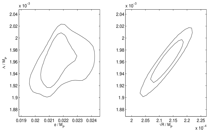
Figure 4: Two-dimensional marginalized joint probability distributions (68% and 95% CL) showing the dependence of the scale at which unitarity is violated $\Lambda$ on the value of the background field $\phi$ (left) and on the comoving curvature perturbations ${\cal R}$ (right) as obtained from the fit of the E-inflation model with $m_{Top}$=171.3 GeV and ${\it v}$=246.22 GeV to the WMAP7+SN+BAO data set. All parameters are computed at the Hubble crossing scale $k_{*}$=0.002Mpc^-1.

Finally, we address the question of the violation of perturbative unitarity for E-inflation model. Figure 4 presents the dependence of the scale at which unitarity is violated in this model, $\Lambda\simeq(2H^{2}\kappa)^{1/3}$, on the value of the background field $\phi$ and on the comoving curvature perturbations ${\cal R}\simeq 12H^{2}$, as obtained from the MCMC analisys. We find that $\Lambda$ is smaller than both $\sqrt{R}$ and $\phi$ during E-inflation, confirming that this model suffers from unitarity problems [27], contrary to the original claims [26].

Table 1: Mean values and the lower and upper intervals (at 68% CL) of parameters obtained from the fit of the SM Higgs inflation variants with $m_{Top}$=171.3 GeV and ${\it v}$=246.22 GeV to the WMAP7+SN+BAO data set. All parameters are computed at the Hubble radius crossing $k_{*}$=0.002 Mpc^-1.

Model	$\zeta$-inflation	G-inflation	E-Inflation
Parameter
$100\Omega_{b}h^{2}$	2.257${}_{2.206}^{2.308}$	2.272${}_{2.247}^{2.296}$	2.254${}_{2.294}^{2.315}$
$\Omega_{c}h^{2}$	0.114${}_{0.111}^{0.117}$	0.117${}_{0.113}^{0.123}$	0.118${}_{0.114}^{0.121}$
$\tau$	0.086${}_{0.073}^{0.093}$	0.094${}_{0.083}^{0.109}$	0.091${}_{0.081}^{0.109}$
$\theta_{s}$	1.037${}_{1.035}^{1.039}$	1.039${}_{1.038}^{1.041}$	1.040${}_{1.039}^{1.044}$
$m_{Higgs}$(GeV)	155.37${}_{151.52}^{159.22}$	143.83${}_{134.87}^{152.98}$	151.578${}_{147.76}^{156.46}$
$\zeta\times 10^{-4}$	3.147${}_{2.638}^{3.656}$	…	…
$w/M_{P}$	…	6.58${}_{6.22}^{6.93}$ $\times 10^{-6}$	4.369${}_{4.194}^{4.522}\times 10^{8}$
${\cal N}$	$58.88^{59.64}_{58.26}$	$59.01_{58.13}^{59.79}$	$58.87_{57.86}^{59.68}$
${\rm ln}[10^{10}A^{2}_{S}]$	3.161${}_{3.129}^{3.193}$	3.177${}_{3.154}^{3.203}$	3.151${}_{3.124}^{3.188}$
$n_{S}$	0.972${}_{0.9716}^{0.9722}$	0.968${}_{0.9597}^{0.9690}$	0.975${}_{0.9741}^{0.9795}$
$n_{T}\times 10^{2}$	-0.0442${}_{-0.0463}^{-0.0421}$	-1.575${}_{-1.592}^{-1.560}$	-1.023${}_{-1.028}^{-1.018}$
R	0.0036${}_{0.0027}^{0.0045}$	0.137${}_{0.134}^{0.140}$	0.041${}_{0.0387}^{0.0421}$

5 CONCLUSIONS

Although the SM Higgs inflaton non-minimally coupled to gravity can account for inflation ($\zeta$-inflation), other variants of Higgs inflation within the SM based on scalar field theories with non-canonical kinetic term such as Galileon-like kinetic term (G-inflation) and kinetic term with non-minimal derivative coupling to the Einstein tensor (E-inflation) have been proposed. In this paper we have analyzed the possibility to distinguish $\zeta$-inflation, G-inflation and E-inflation models through their predictions for $n_{S}$ and $R$ as a function of $m_{Higgs}$ as well as through their predictions for the consistency relations.
In order to ensure consistent results, we have studied the SM Higgs inflation variants considering the full dynamics of the background and perturbations of the Higgs field during inflation and compute the RG improved Higgs potential by including the two-loop $\beta$-functions for the SU(2) $\times$ SU(1) gauge couplings, the SU(3) strong coupling, the top Yukawa coupling, the Higgs quadratic coupling and the Higgs field anomalous dimension. Assuming that all SM Higgs inflation variants are consistent theories, we use the MCMC technique to derive constraints on the inflationary parameters and the Higgs boson mass from their fit to WMAP7+SN+BAO data set. We show that the SM Higgs inflation variants lead to significant constraints on $n_{s}$, $R$ and $m_{Higgs}$.
From the analysis of the confidence regions in $n_{S}$-$m_{Higgs}$ plane we conclude that in order to discriminate the SM Higgs inflation variants by using these parameters the measurement by LHC of $m_{Higgs}$ and an improved detection of $n_{S}$ are required. If PLANCK satellite, designed to measure $n_{S}$ to an accuracy of $4\times 10^{-4}$, will find $n_{S}$ smaller then 0.97, while LHC will find a Higgs mass significantly smaller then 151 GeV, the $\zeta$-inflation and $E$-inflation models would be ruled out.
We also find a striking difference for the predicted values for $R$ by different models. While for $E$-inflation and $\zeta$-inflation the predicted values for $R$ are low, the G-inflation model predicts $R$ values enough large to be detected by the PLANCK satellite. We conclude that if PLANCK will detect a value of $R\sim 0.1$ while LHC will find a Higgs mass significantly smaller then 151 GeV, the $\zeta$-inflation and $E$-inflation models would be ruled out.
We also show that the consistency relations are distinct enough to differentiate the SM Higgs inflation variants.

6 Appendix

In this appendix we collect the SM renormalization group $\beta$-functions at renormalization energy scale $t={\rm ln}(\phi/m_{Top})$ beyond the top quark mass $m_{TOP}$.
All $\beta$-functions and the Higgs field anomalous dimension $\gamma$ include the Higgs field suppression factor $s(t)$ that for the case of $\zeta$-inflation is given by [4, 38]:

$$s(t)=\frac{1+\zeta(t)\phi^{2}(t)}{1+(6\zeta(t)+1)\zeta(t)\phi^{2}(t)}\,.$$ (6.1)

For the case of G-inflation and E-inflation we take $s(t)=1$.

The two-loop $\beta$-functions for gauge couplings $g_{i}=\{g^{\prime},g,g_{s}\}$ are [7]:

$$\beta_{g_{i}} = \kappa g_{i}^{3}b_{i}+\kappa^{2}g_{i}^{3}\left[\sum_{j=1}^{3}B_{ij}g_{j}^{2}-s(t)d_{i}^{t}y_{t}^{2}\right],$$ (6.2)

where $\kappa=1/16\pi^{2}$ and

$$b=((40+s(t))/6,-(20-s(t))/6,-7),\quad B = \left(\begin{array}[]{ccc}199/18&9/2&44/3\\ 3/2&35/6&12\\ 11/6&9/2&-26\end{array}\right),$$ (6.6)

$$d^{t}=(17/6,3/2,2).$$ (6.7)

For the top Yukawa coupling $y_{t}$, the two-loop $\beta$-function is given by [4]:

$$\beta_{y_{t}} =\kappa\,y_{t}\left[-\frac{9}{4}g^{2}-\frac{17}{12}g^{\prime 2}-8g^{2}_{s}+\frac{9}{2}s(t)y_{t}^{2}\right]+\kappa^{2}y_{t}\Bigg{[}-\frac{23}{4}g^{4}-\frac{3}{4}g^{2}g^{\prime 2}+\frac{1187}{216}g^{\prime 4}+9g^{2}g_{s}^{2}$$

$$+ \frac{19}{9}g^{\prime 2}g_{s}^{2}-108g_{s}^{4}+\left(\frac{225}{16}g^{2}+\frac{131}{16}g^{\prime 2}+36g_{s}^{2}\right)s(t)y_{t}^{2}+6\left(-2s^{2}(t)y_{t}^{4}-2s^{3}(t)y_{t}^{2}\lambda+s^{2}(t)\lambda^{2}\right)\Bigg{]}\,.$$

The two-loop $\beta$-function for the Higgs coupling $\lambda$ is [4, 38]:

$$\beta_{\lambda} = \kappa\left[(18s^{2}(t)+6)\lambda^{2}-6y_{t}^{4}+\frac{3}{8}\left(2g^{4}+\left(g^{2}+g^{\prime 2}\right)^{2}\right)+\left(-9g^{2}-3g^{\prime 2}+12y_{t}^{2}\right)\lambda\right]$$ (6.9)

$$+ \kappa^{2}\Bigg{[}\frac{1}{48}\left(915g^{6}-289g^{4}g^{\prime 2}-559g^{2}g^{\prime 4}-379g^{\prime 6}\right)+30s(t)y_{t}^{6}-y_{t}^{4}\left(\frac{8g^{\prime 2}}{3}+32g_{s}^{2}+3s(t)\lambda\right)$$

$$+ \lambda\left(-\frac{73}{8}g^{4}+\frac{39}{4}g^{2}g^{\prime 2}+\frac{629}{24}s(t)g^{\prime 4}+108s^{2}(t)g^{2}\lambda+36s^{2}(t)g^{\prime 2}\lambda-312s^{4}(t)\lambda^{2}\right)$$

$$+ y_{t}^{2}\left(-\frac{9}{4}g^{4}+\frac{21}{2}g^{2}g^{\prime 2}-\frac{19}{4}g^{\prime 4}+\lambda\left(\frac{45}{2}g^{2}+\frac{85}{6}g^{\prime 2}+80g_{s}^{2}-144s^{2}(t)\lambda\right)\right)\Bigg{]}.$$

The $\beta$-function for non-minimal coupling $\zeta$ is given by [38]:

$$\beta_{\zeta}=\kappa\left(\zeta+\frac{1}{6}\right)\left(6(1+s(t))\lambda+6y^{2}_{t}-\frac{3}{2}g^{\prime 2}-\frac{9}{2}g^{2}\right)\,.$$ (6.10)

Finally, the two-loop Higgs field anomalous dimension $\gamma$ is given by [4]:

$$\gamma = -\kappa\left[\frac{9g^{2}}{4}+\frac{3g^{\prime 2}}{4}-3y_{t}^{2}\right]-\kappa^{2}\left[\frac{271}{32}g^{4}-\frac{9}{16}g^{2}g^{\prime 2}-\frac{431}{96}s(t)g^{\prime 4}\right]$$ (6.11)

$$+ \kappa^{2}\left[-\left(\frac{45}{8}g^{2}+\frac{85}{24}g^{\prime 2}+20g_{s}^{2}\right)y_{t}^{2}+\frac{27}{4}s(t)y_{t}^{4}-6s^{3}(t)\lambda^{2}\right]\,,$$

References

- [1] F. Bezrukov, & M. Shaposhnikov, ”The Standard Model Higgs boson as the inflaton” Phys. Lett. B 659, 703 (2008), [arXiv:0710.3755 [hep-th]]
- [2] A. O. Barvinsky, A. Yu. Kamenshchik, A. A. Starobinsky, ”Inflation scenario via the Standard Model Higgs boson and LHC”, JCAP 11, 021 (2008) [arXiv:0809.2104 [hep-ph]]
- [3] F. L. Bezrukov, A. Magnin, M. Shaposhnikov, ” Standard Model Higgs boson mass from inflation”, Phys. Lett. B 675, 88 (2009) [arXiv:0812.4950 [hep-ph]]
- [4] de Simone, A., Hertzberg, M. P., Wilczek, F. 2009, ”Running inflation in the Standard Model”, Phys. Lett. B 678, 1 [arXiv:0812.4946 [hep-ph]]
- [5] F. Bezrukov, D. Gorbunov, M. Shaposhnikov, ”On initial conditions for the hot big bang”. JCAP 06, 029 (2009) [arXiv:0812.3622 [hep-ph]]
- [6] A. O. Barvinsky & A. Yu. Kamenshchik, ”Quantum scale of inflation and particle physics of the early universe”, Phys. Lett. B 332, 270 (1994) [arXiv:gr-qc/9404062]
- [7] J. R. Espinosa, G. F. Giudice, A. Riotto, A. ”Cosmological implications of the Higgs mass measurement”, JCAP 05, 002 (2008) [arXiv:0710.2484]
- [8] J. L. F. Barbón & J. R. Espinosa, ”On the Naturalness of Higgs inflation”, Phys. rev. D 79, 081302 (2009) [arXiv:0903.0355 [hep-ph]]
- [9] C. P. Burgess, H. M. Lee, M. Trott, ”Power-counting and the validity of the classical approximation during inflation”, JHEP 09, 103 (2009) [arXiv:0902.4465 [hep-ph]]
- [10] R. N. Lerner & J. McDonald, J. 2010, ”Higgs inflation and naturalness”, JCAP 04, 015 (20010) [arXiv:0912.5463 [hep-ph]] !naturalness
- [11] R. N. Lerner & J. McDonald, J., ”A unitarity-conserving Higgs inflation model”, Phys. Rev. D 82, 103525 (2010) [arXiv:1005.2978 [hep-ph]]
- [12] C. P. Burgess, H. M. Lee, M. Trott, ”On Higgs inflation and naturalness”, JHEP 07, 007 (2010) [arXiv:1002.2730 [hep-ph]]
- [13] M. P. Hertzberg, ”On inflation with non-minimal coupling”, JHEP 11, 023 92010) [arXiv:1002.2995 [hep-ph]]
- [14] F. Bezrukov, A. Magnin, M. Shaposhnikov, S. Sibiryakov, ”Higgs inflation: consistency and generalisations”, JHEP 01, 016 (2011) [arXiv:1008.5157 [hep-ph]]
- [15] S, Ferrara, R. Kallosh, A. Linde, A. Marrani, A. van Proeyen, ”Superconformal symmetry, NMSSM, and inflation”, Phys. Rev. D. 83 025008 (2011), [arXiv:1008.2942 [hep-th]]
- [16] M. Atkins & X. Calmet, ”On the unitarity of linearized General Relativity coupled to matter”, Phys. Lett. B 697, 37 (2011) [arXiv:1002.0003 [hep-th]]
- [17] C. Armendáriz-Picon, T. Damour, V. Mukhanov, ”k-Inflation”, Phys. Lett. B 209 (1999) [arXiv:hep-th/9904075]
- [18] M. Alishahiha, E. Silverstein, D. Tong, ”DBI in the sky: Non-Gaussianity from inflation with a speed limit”, Phys. rev. D 70, 123505 (2004) [arXiv:hep-th/0404084]
- [19] D.A. Easson, S. Mukohyama & B.A. Powell, ”Observational signatures of gravitational couplings in DBI inflation”, Phys. Rev. D 81, 023512 (2010) [arXiv:0910.1353 [astro-ph.CO]]
- [20] L. Amendola, ”Cosmology with nonminimal derivative couplings”, Phys. Lett. B 301 175 (1993) [arXiv:gr-qc/9302010]
- [21] S. Capozziello, G. Lambiase, ”Nonminimal Derivative Coupling and the Recovering of Cosmological Constant”, Gen. Rel. Grav. 31, 1005 (1999) [arXiv:gr-qc/9302010]
- [22] S. Capozziello, G. Lambiase, H.-J.Schmidt, ”Nonminimal Derivative Couplings and Inflation in Generalized Theories of Gravity”, Annalen Phys. 9, 39 (2000) [arXiv:gr-qc/9302010]
- [23] L. N. Granda, ”Non-minimal Kinetic coupling to gravity and accelerated expansion”, JCAP 07, 006 (2010) [arXiv:0911.3702 [hep-th]]
- [24] L. N. Granda, W. Cardona, ”General non-minimal kinetic coupling to gravity”, JCAP 07, 021 (2010) [arXiv:1005.2716 [hep-th]]
- [25] C. Germani & A. Kehagias ”New Model of Inflation with Nonminimal Derivative Coupling of Standard Model Higgs Boson to Gravity”, Phys. Rev. Lett. 105, 011302 (2010) [arXiv:1003.2635 [hep-ph]]
- [26] C. Germani & A. Kehagias, A. ”Cosmological perturbations in the new Higgs inflation”, JCAP 05, 019 (2010) [arXiv:1003.4285 [astro-ph.CO]]
- [27] M. Atkins & X. Calmet, ”Remarks on Higgs inflation”, Phys. Lett. B 697, 37 (2011) [arXiv:1011.4179 [hep-ph]]
- [28] A. Nicolis, R. Rattazzi & E. Trincherini, ”Galileon as a local modification of gravity”, Phys. Rev. D 79, 064036 (2009) [arXiv:0811.2197 [hep-th]]
- [29] C. Deffayet, G. Esposito-Farèse & A. Vikman, ”Covariant Galileon”, Phys. Rev. D, 79 084003 (2009) [arXiv:0901.1314 [hep-th]]
- [30] C. Deffayet, S. Deser & G. Esposito-Farèse, ”Generalized Galileons: All scalar models whose curved background extensions maintain second-order field equations and stress tensors”, Phys. Rev. D, 80, 064015 (2009) [arXiv:0906.1967 [hep-th]]
- [31] T. Kobayashi, T., M. Yamaguchi & J. Yokoyama, ”Inflation Driven by the Galileon Field”, Phys. Rev. Lett. 105, 231302 (2010) [arXiv:1008.0603 [hep-th]]
- [32] K. Kamada, T. Kobayashi, M. Yamaguchi, J. Yokoyama, ”Higgs G inflation”, Phys. Rev. D 83, 083515 (2010) [arXiv:1012.4238 [astro-ph.CO]]
- [33] P. Creminelli, A. Nicolis & E. Trincherini ”Galilean genesis: an alternative to inflation”, JCAP 11, 021 (2010) [arXiv:1007.0027 [hep-th]]
- [34] S. Mizuno & K. Koyama, ”Primordial non-Gaussianity from the DBI Galileons”, Phys. Rev. D 82 103518 (2010) [arXiv:1009.0677 [hep-th]]
- [35] C. Burrage, C. de Rham, D. Seery, A. Tolley, ”Galileon inflation”, JCAP 01, 014 (2011) [arXiv:1009.2497 [hep-th]]
- [36] A. De Felice & S. Tsujikawa, ”Primordial non-gaussianities in general modified gravitational models of inflation”, JCAP 04, 029 (2011) [arXiv:1103.1172 [astro-ph.CO]]
- [37] T. Kobayashi, M. Yamaguchi, & J. Yokoyama, ”Primordial non-Gaussianity from G inflation”, Phys. rev. D 83, 103524 (2011) [arXiv:1008.0603 [hep-th]]
- [38] R. N. Lerner, J. McDonald, ”Distinguishing Higgs inflation and its variants”, Phys. Rev. D 83, 123522 (2011) [arXiv:1104.2468 [hep-ph]]
- [39] L.A. Popa & A. Caramete, ”Cosmological Constraints on the Higgs Boson Mass”, ApJ 723, 803 (2010) [arXiv:1009.1293 [astro-ph.CO]]
- [40] A. De Felice, S. Tsujikawa, J. Elliston, R. Tavakol, ”Chaotic inflation in modified gravitational theories” (2011) [arXiv:1105.4685 [astro-ph.CO]]]
- [41] T. Futamase, & K. Maeda, ”Chaotic inflationary scenario of the Universe with a nonminimally coupled “inflaton” field”, Phys. Rev. D 39, 399 (1989)
- [42] E. Komatsu, & T. Futamase, ”Constraints on the chaotic inflationary scenario with a nonminimally coupled “inflaton” field from the cosmic microwave background radiation anisotropy”, Phys. Rev. D 58, 023004 (1998) [arXiv:astro-ph/9711340].
- [43] E. Komatsu & T. Futamase, ”Complete constraints on a nonminimally coupled chaotic inflationary scenario from the cosmic microwave background”, Phys. Rev. D 59, 064029 (1999) [arXiv:astro-ph/9901127]
- [44] S. Tsujikawa & B. Gumjudpai, ”Density perturbations in generalized Einstein scenarios and constraints on nonminimal couplings from the cosmic microwave background”, Phys. Rev. D 69, 123523 (2004) [arXiv:astro-ph/0402185]
- [45] E. Komatsu, et al. (WMAP Collaboration), ”Seven-Year Wilkinson Microwave Anisotropy Probe (WMAP) Observations: Cosmological Interpretation”, ApJS 192, 18 (2011) [arXiv:1001.4538 [astro-ph.CO]]
- [46] D. Larson et al. (WMAP Collaboration) ”Seven-Year Wilkinson Microwave Anisotropy Probe (WMAP) Observations: Power Spectra and WMAP-Derived Parameters”, ApJS 192, 16 (2011) [arXiv:1001.4635 [astro-ph.CO]]
- [47] J. Garriga & V. F. Mukhanov, ”Perturbations in k-inflation”, Phys. Lett. B 458, 219 (1999) [arXiv:hep-th/9904176]
- [48] K. Nakamura et al., ”The Review of Particle Physics” J. Phys. G 37, 075021 (2010)
- [49] A. O. Barvinsky, A. Yu. Kamenshchik, C. Kiefer, A. A. Starobinsky, C. F. Steinwach ”Asymptotic freedom in inflationary cosmology with a non-minimally coupled Higgs fields”, JCAP 12, 003 (2009) [arXiv:0904.1698 [hep-ph]]
- [50] D. H. Lyth & A. A. Riotto, ”Particle physics models of inflation and the cosmological density perturbation”, Phys. Rep. 314, 1 (1999) [arXiv:hep-ph/9807278]
- [51] A. Lewis, A. Challinor & A. Lasenby, ”Efficient Computation of Cosmic Microwave Background Anisotropies in Closed Friedmann-Robertson-Walker Models”, ApJ 538, 473 (2000) 111http://camb.info [arXiv:astro-ph/9911177]
- [52] A. Lewis & S. Briddle S., Phys. Rev. D 66, 103511 (2002) 222http://cosmologist.info/cosmomc/ [arXiv:astro-ph/0205436]
- [53] W. H. Kinney, E. W. Kolb, A. Melchiorri, A. Riotto, ”Inflationary physics from the Wilkinson Microwave Anisotropy Probe”, Phys. Rev D 69, 103516 (2004) [arXiv:hep-ph/0305130]
- [54] W. H. Kinney & A. Riotto, ”Theoretical uncertainties in inflationary predictions”, JCAP 03 011 (2006) [arXiv:astro-ph/0511127]
- [55] J. Garcia-Bellido, D. G. Figueroa & J. Rubio, ”Preheating in the standard model with the Higgs inflaton coupled to gravity”, Phys. Rev. D 79, 063531 (2009) [arXiv:0812.4624 [hep-ph]]
- [56] M. Kowalski et al. (Supernova Cosmology Project), ”Improved Cosmological Constraints from New, Old, and Combined Supernova Data Sets”, ApJ 686, 749 (2008) [arXiv:0804.4142 [astro-ph]]
- [57] Riess et al., ”A Redetermination of the Hubble Constant with the Hubble Space Telescope from a Differential Distance Ladder”, ApJ 699, 539 (2009) [arXiv:0905.0695 [astro-ph.CO]]
- [58] W. J. Percival, et al., ”Baryon acoustic oscillations in the Sloan Digital Sky Survey Data Release 7 galaxy sample”, MNRAS 401, 2148 (2010) [arXiv:0907.1660 [astro-ph.CO]]
- [59] A. Gelman & D. Rubin, Statistical Science 7, 457 (1992)
- [60] F. Bezrukov, D. Gorbunov, ”Light inflaton hunter’s guide”, JHEP 05, 010 (2010) [arXiv:0912.0390 [hep-ph]]
- [61] C. Deffayet, O. Pujolas, I. Sawicki, A. Alexander, ”Imperfect dark energy from kinetic gravity braiding”, JCAP 10, 026 (2010) [arXiv:1008.0048 [hep-th]]