Seismic diagnostics for rotating massive main sequence stars

Abstract

Effects of stellar rotation on adiabatic oscillation frequencies of $\beta$ Cephei star are discussed. Methods to evaluate them are briefly described and some of the main results for four specific stars are presented.

1 Introduction

Main sequence (MS) massive stars are usually fast rotators and their fast rotation affects their internal structure as well as their evolution. The issue which is adressed here is what information can we obtain- about rotation - from the oscillations of these massive, main sequence stars ?

The following seismic diagnostics for rotation using non axisymmetric modes will be discussed: 1) rotational splittings as direct probes of the rotation profile. More precisely, we study the effects of cubic order in the rotation rate compared to effects of a latitudinal dependence of the rotation on the splittings; 2) splitting asymmetries as a probe for centrifugal distorsion. The case of 3) axisymmetric modes as indirect probes of rotation throughout effect of rotationally induced mixing on the structure will also be considered.

Results discussed here are obtained with perturbation methods. For nonperturbative methods and results, we refer the reader to Lignières et al. (2006), Reese et al. (2009) and references therein.

The paper is organized as follows: in Sect.2, properties of pulsating B stars are recalled with emphasis on the uncertainties of their physical description that can be addressed by seismic analyses. Sect. 3. recalls the theoretical framework for seismic analyses of relevance here. In Sect.4, seismic analyses of four $\beta$ Cep are presented. In Sect.5 a theoretical study compares the modifications of the rotation splittings due either to latitudinal dependence of the rotation rate, $\Omega$, or to cubic order ($O(\Omega^{3}$)) frequency corrections. Some conclusions are given in Sect.6.

2 Massive main sequence stars

O-B stars are characterized by a convective core and an envelope which is essentially radiative apart a thin outer region related to the iron opacity bump. Important incertainties regarding the structure and future evolution of these stars are:
-the extent of chemical element mixing beyond the central instable layers as defined by the Schwarzschild criterium
-Transport of angular momentum because the rotation can play a significant role in chemical element mixing

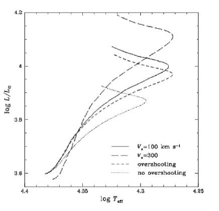
Figure 1: Evolutionary tracks for $9M_{\odot}$ models with neither rotation, nor overshoot included (dotted line), with overshoot included but not rotation (short dashed line) and with rotation included but not overshoot (long dashed and solid lines) (from Talon et al., 1997)

Convective core overshoot: In 1D stellar models, the convective core is delimited by the radius $r_{zc}$ according to the Schwarzschild criterium $\nabla_{ad}=\nabla_{rad}$. However this corresponds to a vanishing buoyancy force: the eddies are then strongly slowed down but still retain some velocity. Hence due to inertia, eddies move beyond the Schwarzschild radius till their velocity vanishes that-is over a distance $d_{ov}$ such that the effective convective core radius becomes $r_{ov}=r_{zc}+d_{ov}$. Despite theoretical investigations (Zahn, 1991, Roxburgh, 1992), the overshooting distance computed in 1D stellar evolutionary models usually remains a rough prescription i.e. it is assumed that $d_{ov}=\alpha_{ov}{\rm min}(r_{zc},H_{p})$ with $H_{p}$ the local pressure scale height and $\alpha_{ov}$ is a free parameter. Empirical determinations from observations (Schaller et al. 1992, Cordier et al. 2002; Claret, 2007 and references therein) yield a wide range for $\alpha_{ov}$, namely [0-0.5] $H_{p}$. The adopted value for this free parameter has important consequences for the evolution of a model with a given mass: with a higher luminosity, it is older at given central hydrogen content ($X_{c}$) on the MS and reaches the end of the MS with a larger mass core- total mass ratio. On a statistical point of view, the value of $\alpha_{ov}$ affects the thickness of the MS on a HR diagram as well as the isochrones. Core overshoot has therefore an influence on stellar age determination (Lebreton et al. 1995, Lebreton, 2008).

Rotationally induced mixing in radiative regions: Departure from thermal equilibrium generated by the oblateness of a rotating star causes large scale motions, the meridional circulation. As differential rotation also induces turbulence, competition of these two processes can result in (rotationally induced) diffusion of chemical elements (Zahn, 1992 and subsequent works). The evolution of a given chemical specie $j$ with concentration $c_{j}$ is governed by a diffusion equation (for a review, Talon, 2008; Decressin et al. 2009):

$$\rho{dc_{j}\over dt}=\rho\dot{c}_{j}+{1\over r^{2}}{\partial\over\partial r}[r^{2}\rho V_{ip}]+{1\over r^{2}}{\partial\over\partial r}[r^{2}\rho D_{t}{\partial c_{j}\over\partial r}]$$ (1)

where the first term represents nuclear transformation and the second term atomic diffusion with $V_{j,p}$ the diffusion velocity of particles j with respect to protons and where the tuirbulent diffusion coefficient $D_{t}=D_{eff}+D_{v}$, $D_{eff}$ comes from the meridional circulation and $D_{v}$ from the turbulence. As $D_{eff}$ depends on the vertical meridional velocity $U_{r}$, chemical and angular momentum evolutions must be solved together. Hence one also solves an (diffusion-advection) evolution equation for the angular momentum :

$$\rho{dr^{2}\Omega\over dt}={1\over 5r^{2}}{\partial\over\partial r}[r^{4}\rho\Omega U_{r}]+{1\over r^{4}}{\partial\over\partial r}[r^{4}\rho\nu_{v}{\partial\Omega\over\partial r}]$$ (2)

where $\nu_{v}$ is the vertical turbulent viscosity related to rotational instabilities. The current picture is that the vigor of the meridional circulation is controlled by the magnitude of the surface losses of angular momentum. Hence for hot, high mass stars which lose mass but much less angular momentum, one expects no efficient angular momentum internal transport. The rotation profile then essentially results from expansion and contraction within the star during its evolution: i.e. high ratio of core rotation over surface rotation. This is well reproduced by rotationally induced mixing of type I (Talon et al. 1997). On the other hand, for cool stars with extended convective outer layers, dynamo generates an efficient magnetic driven wind which is efficient to drive important angular momentum losses and internal transport. This mechanism however is not sufficient enough in the solar case to make the observed rigid rotation in the radiative solar interior and one must calls for to other mechanisms (waves, magnetic field) (see Talon, 2007; Rieutord, 2006 for reviews). This shows that many open questions related to stellar internal rotation and its gradients subsist. An important issue then is to locate regions of uniform rotation and regions of differential rotation (depth and/or latitude dependence) inside the star ($\Omega_{core}/\Omega_{surf}$). Another problem which must be solved is to disentangle effects of overshooting and rotation on mixed central regions and extension of convective cores. Indeed the rotationally induced chemical mixing affects the evolution of the star, its internal structure and oscillation frequencies as does core overshoot although in a different way (Talon et al., 1997; Goupil & Talon, 2002; Montalban et al., 2008; Miglio et al., 2008; Thoul, 2009). Fig.1 illustrates the respective effects of element mixing by core overshoot and rotation on the evolution of a 9 $M_{\odot}$ main sequence model in a HR diagram.

Seismology of O-B stars can bring some light about these processes. More specifically, $\beta$ Cephei stars are good candidates for this purpose (Montalban et al., 2008; Miglio et al., 2008; Goupil & Talon, 2008; Miglio et al., 2009; Lovekin et al., 2008; Lovekin & Goupil, 2009). Indeed, unlike $\delta$ Scuti stars, $\beta$ Cephei stars do not present significant outer convective layers which makes the mode identification more trustworthy provided the star is slowly rotating or that its fast rotation is taken into account in the mode identification process (Lignières et al., 2006, Reese et al., 2009; Lovekin et al. 2008; Lovekin et al. 2009).

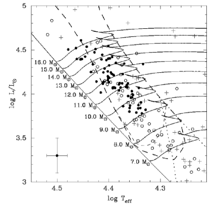
Figure 2: left: HR diagram and instability strip for beta Cephei stars. Full dots represent confirmed $\beta$ Cephei stars and open dots : candidates. The dashed lines delimitate the instability strip for the fundamental radial mode (adapted from Stankov & Handler 2005).

2.1 $\beta$ Cephei stars

$\beta$ Cephei stars are main sequence stars with masses roughly larger than $5-7M_{\odot}$ (Fig. 2). They oscillate with a few low degree, low radial order modes around the fundamental radial mode i.e. with periods around 3-8 h. The modes are excited by the kappa mechanism due to the iron bump opacity. These pulsating stars are located at the intersection of the main sequence and their instability strip in a HR diagram (Fig.2). For more details about $\beta$ Cephei stars, we refer to reviews by Handler (2006), Stankov & Handler (2005), Pigulski (2007), Aerts (2008).

Figure 3: Propagation diagram for model A: a 8.5 $M_{\odot}$ model with $T_{eff}=22230K$ and initial $X=0.7,Z=0.019$ (no rotation, no overshoot). The Lamb frequency (dashed line) is plotted for $\ell=1$. Normalized squared frequencies discussed here are found in the range $\sigma^{2}$=5-15.

Sofar the observed modes have been identified as p1, p2, g1 modes. We recall that p modes are propagative when $\omega^{2}>N^{2}$ and $\omega^{2}>S_{l}^{2}$ (for more details, see Christensen-Dalsgaard, 2003 CD03). The squared Brünt-Väissälä (buoyancy) frequency is defined as

$$N^{2}={g\over r}~{}\Bigl{(}{1\over\Gamma_{1}}{d\ln p\over d\ln r}-{d\ln\rho\over d\ln r}\Bigr{)}$$ (3)

with $p,\rho,g$ respectively the pressure, density and gravity of the stellar medium and $\Gamma_{1}$ the adiabatic index. The squared Lamb frequency is defined as

$$S_{l}^{2}=(k_{h}c_{s})^{2}=\ell(\ell+1){c_{s}^{2}\over r^{2}}$$ (4)

with $k_{h}$ the horizontal wavenumber of the pulsation mode and $\ell$ the degree of the mode (when its surface distribution is described with a spherical harmonics $Y_{\ell}^{m}(\theta,\phi)$). The local sound speed $c_{s}$ is given by:

$$c_{s}=\Bigl{(}{\Gamma_{1}p\over\rho}\Bigr{)}^{1/2}$$ (5)

For g-modes, the propagative region is delimitated by $\omega^{2}<N^{2}$ and $\omega^{2}<S_{l}^{2}$.

For $\beta$ Cephei stars, mixed modes propagate as g mode in the inner part and as p mode in the outer part of the star. Depending on the evolutionary stage of the star, one expects some of the detected modes to be of mixed p and g nature. Modes with frequencies around that of the fundamental radial one (normalized frequency $\sigma=\omega/\Omega_{K}\sim 2-3$ with $\Omega_{K}=(GM/R^{3})^{1/2}$, $R$ the radius and $M$ the mass of the star) can be mixed modes. This can be seen in Fig.3 which shows a propagation diagram for a typical case, model A, a model with a mass 8.5 $M_{\odot}$ and an age $=19.9~{}Myr$, a solar metallicity to hydrogen ratio $Z/X=0.019$ with $X=0.7$ and $\log~{}T_{eff}=4.347$ and $\log~{}L/L_{\odot}=3.723$ that therefore lies in the middle of the main sequence and instability strip for these stars.

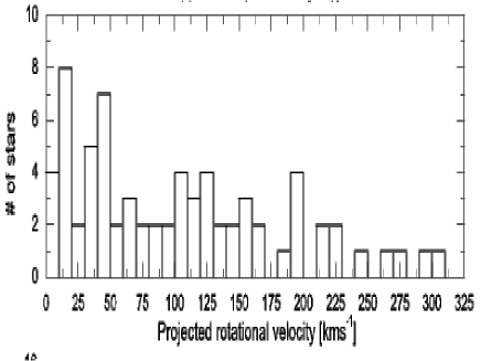
Figure 4: Histogram of projected rotational velocities for $\beta$ Cephei stars (from Stankov, Handler 2005).

Rotation of $\beta$ Cephei stars ranges from slow (rotational velocity $v<50$ km/s) to extremely rapid ($v>250$ km/s) (Fig.4). Effects of uniform rotation start to modify significantly the tracks in a HR diagram beyond $v=100$ km/s for these masses (Lovekin et al., 2009). For $v=100$ km/s, with a stellar radius $R=4.94R_{\odot}$, model A is characterized by $\Omega/\Omega_{K}\sim 0.175$ where $\Omega_{K}=(GM/R^{3})^{1/2}$ is the break up angular velocity.

3 Theoretical framework

In this section, we recall the theoretical framework within which seismic observations of these stars can be interpreted in terms of rotation (for more details, the reader is referred to Goupil (2009) and references therein). For sake of notation, we recall first the non rotating case.

3.1 No rotation

Adiabatic pulsation studies consider the linearized conservation equations for a compressible, stratified fluid about a static equilibrium stellar model characterized by $P_{0},\rho_{0},\Gamma_{1},\phi_{0}$ respectively pressure, density, adiabatic index, gravitational potential profiles. The equation for hydrostatic equilibrium is :

$$\vec{\nabla}p_{0}=-\rho_{0}~{}\vec{\nabla}\phi_{0}$$ (6)

Assuming the fluid displacement $\vec{\delta r}(\vec{r},t)$ of the form $\vec{\delta r}(\vec{r},t)=\vec{\xi}(\vec{r})~{}exp(i\omega_{0}t)$, the linearized momentum equation then is:

$${\cal L}_{0}(\vec{\xi})-\rho_{0}~{}\omega_{0}^{2}~{}\vec{\xi}=0$$ (7)

with

$${\cal L}_{0}(\vec{\xi})\equiv\nabla p^{\prime}+\rho_{0}\nabla\phi^{\prime}+\rho^{\prime}\nabla\phi_{0}$$

where ${\cal L}_{0}$ is a differential operator acting on $\vec{\xi}$; $p^{\prime},\rho^{\prime},\phi^{\prime}$ are the Eulerian perturbation for the pressure, density and gravitational potential respectively. One must add boundary conditions (Unno et al., 1989) and this gives rise to an eigenvalue problem where $\omega_{0}$ is the eigenvalue for the nonrotating case and $\vec{\xi}$ is the eigenfunction for the fluid displacement. In the following, we will keep the notation: $\nu$ in $\mu$Hz or c/d ; $\omega$ in rad/s; $\sigma=\omega/(GM/R^{3})^{1/2}$ the normalized frequency. One defines the scalar product:

$$<\vec{a}|\vec{b}>\equiv\int_{V}~{}\vec{a}^{*}\cdot\vec{b}~{}{\bf d^{3}r}$$ (8)

where $*$ means complex conjugate and where $V$ is the stellar volume. The scalar product of $\vec{\xi}$ with Eq.7 then yields:

$$<\vec{\xi}|{\cal L}_{0}(\vec{\xi})-\rho_{0}\omega_{0}^{2}\vec{\xi}>\equiv\int_{V}~{}\vec{\xi}^{*}\cdot({\cal L}_{0}(\vec{\xi})-\rho_{0}\omega_{0}^{2}\vec{\xi})~{}{\bf d^{3}r}=0$$

The eigenfrequency can be obtained as an integral expression:

$$\omega_{0}^{2}={1\over I}<\vec{\xi}|{\cal L}_{0}(\vec{\xi})>$$ (9)

or

$$\omega_{0}^{2}={1\over I}\int_{V}~{}\vec{\xi}^{*}\cdot(\nabla p^{\prime}+\rho_{0}\nabla\phi^{\prime}+\rho^{\prime}\nabla\phi_{0})~{}{\bf d^{3}r}$$ (10)

with

$$I=\int_{V}~{}(\vec{\xi}^{*}\cdot\vec{\xi})~{}\rho_{0}~{}{\bf d^{3}r}$$ (11)

In absence of rotation, the eigenmode displacement is written in a spherical coordinate system with a single harmonics, $Y_{\ell}^{m}(\theta,\phi)$, with a spherical degree $\ell$, an azimuthal number $m$ being the number de nodes along the equator

$$\vec{\xi}(\vec{r})=\xi_{r}(r)~{}Y_{\ell}^{m}~{}\vec{e}_{r}+\xi_{h}(r)~{}\vec{\nabla}_{h}Y_{\ell}^{m}$$ (12)

where the first part is the radial component and the second term the horizontal component of the fluid displacement. The horizontal divergence is

$$\vec{\nabla}_{h}=\vec{e}_{\theta}~{}{\partial\over\partial\theta}+\vec{e}_{\phi}~{}{1\over\sin\theta}{\partial\over\partial\phi}$$

The divergence of the fluid displacement is written as:

$$\vec{\nabla}\cdot\xi=\lambda~{}Y_{\ell}^{m}$$ (13)

with

$$\lambda={1\over r^{2}}{dr^{2}\xi_{r}\over dr}-{\Lambda\over r}~{}\xi_{h}$$ (14)

and $\Lambda=\ell(\ell+1)$. The perturbed density $\rho^{\prime}(\vec{r})=\rho^{\prime}(r)Y_{\ell}^{m}$ is given by the linearized continuity equation:

$$\rho^{\prime}(r) = -\nabla\cdot(\rho_{0}\vec{\xi})=-{d\rho_{0}\over dr}\xi_{r}-\rho_{0}\lambda$$ (15)

The perturbed gravitational potential $\phi^{\prime}(\vec{r})=\phi^{\prime}(r)Y_{\ell}^{m}$ is given by the perturbed Poisson equation:

$$\nabla^{2}\phi^{\prime} = 4\pi G\rho^{\prime}$$ (16)

The pressure perturbation $p^{\prime}(r)$ is related to the density perturbation $\rho^{\prime}(r)$ by the adiabatic relation (Unno et al.1989) where $\delta$ means here a Lagrangean variation:

$${\delta p\over p_{0}}=\Gamma_{1}{\delta p\over p_{0}}$$

3.2 Including rotation

In presence of rotation the centrifugal and Coriolis accelerations come into play. The centrifugal force affects the structure of the star - the star is distorted- and causes a departure from thermal equilibrium which generates large scale meridional circulation and chemical mixing. Accordingly, the resonant cavities of the modes are modified. The static equilibrium (averaged over horizontal surfaces) 1D stellar model is modified and characterized by $P_{0,\Omega}(r),\rho_{0,\Omega}(r),\Gamma_{1,\Omega}(r),\phi_{0,\Omega}(r)$ with $\Omega(r,\theta)$ the rotation rate. The Coriolis force enters the equation of motion and affects the motion of waves and frequencies of normal modes. The linearized equation of motion is modified. As rotation breaks the azimuthal symmetry, it lifts the frequency degeneracy: without rotation, $2\ell+1$ modes with given $n,\ell,m$ ($m=-\ell,\ell$) have the same frequency $\omega_{0}$ (omitting for shortness the subscripts $n,\ell$). With rotation, the same $2\ell+1$ modes have different frequencies $\omega_{m}$ and the rotational splitting is defined as : $S_{m}=(\omega_{m}-\omega_{0})/(m)$. One also uses $S_{m}=\omega_{m}-\omega_{m-1}$ and the generalized rotational splitting:

$$S_{m}={\omega_{m}-\omega_{-m}\over 2m}$$ (17)

where $\omega_{m}$ is the mode frequency. These various definitions are equivalent only at first perturbation order in the rotation rate $\Omega$; the first two are used when only a few components are available.

3.3 Rotational splittings

At first perturbation order in $\Omega$, only the Coriolis acceleration plays a role. The linearized equation of motion including the effect of Coriolis acceleration ($2\Omega\times\vec{v}$) in a frame of inertia is

$${\cal L}_{0}(\vec{\xi})-\rho_{0}~{}(\omega_{m}+m\Omega)^{2}\vec{\xi}+2\rho_{0}~{}(\omega_{m}+m\Omega)~{}\Omega~{}{\cal K}\vec{\xi}=0$$ (18)

with ${\cal K}\vec{\xi}=i\vec{e}_{z}\times\vec{\xi}$ and $\vec{\xi}$ is the displacement eigenvector in absence of rotation and $e_{z}$ is the vectical unit vector in cylindrical coordinates. The nonrotating case is recovered by setting $\Omega=0$. One then expands the displacement eigenfunction as $\vec{\xi}=\vec{\xi}_{0}+\vec{\xi}_{1}$ and the eigenfrezquency as $\omega_{m}=\omega_{\Omega=0}+\omega_{1,m}$ where $\omega_{\Omega=0}$, $\vec{\xi}_{0}$ correspond to the eigenfrequency and eigenfunction for a nonrotating star and $\omega_{1,m}$, $\vec{\xi}_{1}$ give the first order correction due to Coriolis acceleration. Keeping only terms up to $O(\Omega)$, one obtains:

$${\cal L}_{0}(\vec{\xi}_{1}) - \rho_{0}~{}\omega_{\Omega=0}^{2}~{}\vec{\xi}_{1}-2\rho_{0}~{}\omega_{\Omega=0}(\omega_{1,m}+m\Omega)~{}\vec{\xi}_{0}$$ (19)

$$+ 2\rho_{0}~{}\omega_{\Omega=0}~{}\Omega~{}{\cal K}\vec{\xi}_{0}=0$$ (20)

The correction to the eigenfunction $\vec{\xi}_{1}$ can be chosen so that $<\vec{\xi}_{0}|\vec{\xi}_{1}>=0$. Taking the scalar product Eq.8 of $\vec{\xi}_{0}$ with Eq.20 and keeping only terms up to $O(\Omega)$ yields:

$$<\vec{\xi}_{0}|\left[\right.{\cal L}_{0}(\vec{\xi}_{1}) - \rho_{0}~{}\omega_{\Omega=0}^{2}~{}\vec{\xi}_{1}-2\rho_{0}~{}\omega_{\Omega=0}~{}(\omega_{1,m}+m\Omega)~{}\vec{\xi}_{0}$$ (21)

$$+ 2\rho_{0}~{}\omega_{\Omega=0}~{}\Omega~{}{\cal K}\vec{\xi}_{0}\left.\right]>=0$$ (22)

from which one derives for a mode with given $n,\ell$

$$~{}\omega_{1,m}~{}I_{0} = \int_{V}~{}\vec{\xi}_{0}^{*}\cdot(\Omega~{}{\cal K}-m\Omega)~{}\vec{\xi}_{0}~{}\rho_{0}~{}{\bf d^{3}r}$$ (23)

which is rewritten as:

$$\omega_{1,m}=\int_{0}^{R}\int_{0}^{\pi}K_{m}(r,\theta)~{}{\Omega(r,\theta)}~{}d\theta dr$$ (24)

where the analytical expression for the kernels $K_{m}$ is given in Appendix. At first order $O(\Omega)$, the generalized splitting Eq.17 then is given by

$$S_{m}={\omega_{1,m}-\omega_{1,-m}\over 2m}$$ (25)

Assuming a shellular rotation $\Omega(r)$, the splitting $S_{m}$ becomes $m$ independent and one has:

$$S=~{}\int_{0}^{R}~{}K(r)~{}{\Omega(r)}~{}dr$$ (26)

with the rotational kernel

$$K(r)=-{1\over I}\left(\xi_{r}^{2}-2\xi_{r}\xi_{h}+(\Lambda-1)\xi_{h}^{2}\right)~{}\rho_{0}~{}r^{2}$$ (27)

and mode inertia (Eq.11):

$$I=\int_{0}^{R}~{}(\xi_{r}^{2}+\Lambda\xi_{h}^{2})~{}\rho_{0}r^{2}dr$$ (28)

with again $\Lambda=\ell(\ell+1)$ and $R$ the stellar radius. For a uniform rotation, this further simplifies to

$$S=\Omega~{}\beta~{}~{}~{}~{}~{}~{}~{}~{};~{}~{}~{}~{}\beta=\int_{0}^{R}~{}K(r)~{}dr$$ (29)

$\beta$ is assumed to be known from an appropriate stellar model, $S$ is measured and $\Omega$ is inferred. This will be used in Sect.4 for $\beta$ Cep stars.

When only a few measured splittings are available, information about the internal rotation is limited so one assumes for instance a uniform rotation for the convective core with the angular velocity $\Omega=\Omega_{c}$ (for $x=r/R\leq x_{c}$) and a uniform rotation for the envelope $\Omega=\Omega_{e}$ for $x>x_{c}$. Both values are the unknowns. Inserting into Eq.26,

$$S=\int_{0}^{1}K(x)~{}\Omega(x)~{}dx=\Omega_{c}\beta_{c}+\Omega_{e}\beta_{e}$$

with

$$\beta_{c}=\int_{0}^{x_{c}}K(x)~{}dx~{}~{};~{}~{}\beta_{e}=\int_{x_{c}}^{1}K(x)~{}dx$$

The detection of 2 triplets $\ell=1$ for instance yields $\Omega_{c}$, $\Omega_{e}$ and $\Omega_{c}/\Omega_{e}$ provided $\beta_{c},\beta_{e}$ are given by a model close to the observed star. This type of approach was used to determine whether the star is in rigid rotation or not for a $\delta$ Scuti star (Goupil et al., 1993); for white dwarfs (Winget et al. 1994; Kawaler et al., 1999) and recently for $\beta$ Cephei stars (Sect.4 below) and SdB stars (Charpinet et al., 2008).

3.4 Splitting asymmetries: distorsion

At second order in the rotation rate, the centrifugal acceleration comes into play. This has several consequences on the oscillation frequencies (for a review Goupil, 2009). One is that the split components are no longer equally spaced. It is then convenient to define $A_{m}$ the splitting asymmetry as

$$A_{m}=\omega_{0}-{1\over 2}(\omega_{m}+\omega_{-m})$$ (30)

In order to interpret observed asymmetries, let consider a given multiplet of modes (i.e. with specified $n,\ell$). Its oscillation frequencies, $\omega_{m}$ ($m=-\ell,..,\ell$), are computed up to second order $O(\Omega^{2})$ as:

$$\omega_{m}=\omega_{0,\Omega}+m~{}S_{|}m|+{{\bar{\Omega}}^{2}\over\omega_{0,\Omega}}~{}(X_{1}+m^{2}X_{2})$$ (31)

whereand $\omega_{0,\Omega}$ is the eigenfrequency for a static model including the horizontally averaged centrifugal acceleration. The second term is the splitting Eq.25 due to Coriolis effect and ${\bar{\Omega}}$ is an averaged rotation rate. The last term is the asymmetry due to the non spherical part of the centrifugal distorsion which dominates for high radial order modes. Expressions for $X_{1},X_{2}$ can be found in Saio (1981), DG92, Soufi et al. (1998); Suarez et al.(2006); Goupil (2009). For low radial modes such as those excited in $\beta$ Cep stars, the second order Coriolis contributions to $X_{1},~{}X_{2}$ remain significant. According to Eq.31, the asymmetry is then given by:

$$A_{m}=\left({{\bar{\Omega}}^{2}\over\omega_{0,\Omega}}\right)~{}m^{2}~{}X_{2}$$ (32)

Let consider again the linearized equation of motion including now the centrifugal acceleration:

$${\cal L}_{0,\Omega}(\vec{\xi})-\rho_{0,\Omega}~{}\hat{\omega}^{2}~{}\vec{\xi}+2\rho_{0,\Omega}\hat{\omega}\Omega K(\vec{\xi})+{\cal L}_{2}(\vec{\xi})-\rho_{2}~{}\hat{\omega}^{2}~{}\vec{\xi}=0$$ (33)

where $\hat{\omega}=\omega_{m}+m\Omega$. The spherical part of the centrifugal acceleration is included in the spherical 1D model, therefore the linear operator depends on the rotation rate i.e.

$${\cal L}_{0,\Omega}(\vec{\xi})\equiv\nabla p^{\prime}+\rho_{0,\Omega}\vec{\nabla}\phi^{\prime}+\rho^{\prime}\vec{\nabla}\phi_{0,\Omega}$$ (34)

and for the non spherical distorsion

$${\cal L}_{2}(\vec{\xi})=\rho^{\prime}({\rho_{2}\over\rho_{0,\Omega}}\nabla p_{0,\Omega}-\nabla p_{2})+\rho_{2}\nabla\phi^{\prime}+\rho_{0,\Omega}~{}\vec{e}_{s}~{}r\sin\theta~{}\vec{\nabla}\Omega^{2}\cdot\vec{\xi}$$ (35)

where $\vec{e}_{s}=\sin\theta~{}\vec{e}_{r}+\cos\theta~{}\vec{e}_{\theta}$ in a spherical coordinate system ($\vec{e}_{r},\vec{e}_{\theta},\vec{e}_{\phi}$).The subscript 2 indicates departure from sphericity $p_{2},\rho_{2},\phi_{2}$ for the pressure, density and graviational potential respectively. Again using the scalar product Eq.8, one writes

$$<\vec{\xi}_{0}|{\cal L}_{0,\Omega}(\vec{\xi}) - \rho_{0,\Omega}~{}\hat{\omega}^{2}~{}\vec{\xi}+2\rho_{0,\Omega}~{}\hat{\omega}~{}\Omega~{}K(\vec{\xi})>$$ (36)

$$+ <\vec{\xi}|({\cal L}_{2}(\vec{\xi})-\rho_{2}\hat{\omega}^{2}~{}\vec{\xi})>=0$$ (37)

One then assumes an eigenfunction of the form $\vec{\xi}=\vec{\xi}_{0}+\vec{\xi}_{1}+\vec{\xi}_{2}$ and the eigenfrequency as $\omega_{m}=\omega_{0,\Omega}+\omega_{1m}+\omega_{2}$ where the unknown now is $\omega_{2}$. Solving Eq.37 for $\omega_{2m}$ leads to an integral expression for $X_{1},X_{2}$ and therefore an expression for $A_{m}$ of the form:

$$A_{m}=m^{2}\,\int_{0}^{1}~{}\Omega^{2}(x)~{}K_{2}(x)~{}dx$$ (38)

where $K_{2}(x)$ include effects of distorsion of the structure throughout $p_{2},\rho_{2}$ and depend on the eigenfunction $\vec{\xi}$. Detailed expression for $K^{(j)}_{2}(x)$ can be found in DG92, Soufi et al. (1998), Karami (2008), Suarez et al. (2006), Goupil (2009). An exemple for $K_{2}(x)$ is shown in Fig.7 and discussed in Sect.4.2

Splitting asymmetries can provide probes of the internal structure which differ from those derived with the splittings $S_{m}$ as the corresponding kernels are different. When only a few observed asymmetries are available, one can proceed as for the splittings (Sect.3.3 above). Assuming a rotation profile of the simplified form:

$$\Omega^{2}(x) = \Omega_{c}^{2}~{}~{}{\rm for}~{}~{}x_{c}<x$$ (39)

$$\Omega^{2}(x) = \Omega_{c}^{2}+2(x-x_{c})~{}\Omega^{\prime}\Omega_{c}+(x-x_{c})^{2}~{}\Omega^{{}^{\prime}2}~{}~{}{\rm for}~{}~{}x_{c}\leq x\leq x_{e}$$ (40)

$$\Omega^{2}(x) = \Omega_{e}^{2}~{}~{}{\rm for}~{}~{}x_{e}<x$$ (41)

with

$$\Omega^{\prime}={\Omega_{e}-\Omega_{c}\over x_{e}-x_{c}}$$ (42)

then

$$A_{m}=m^{2}\Bigl{(}\Omega_{c}^{2}~{}\beta_{2,0}+2\Omega^{\prime}\Omega_{c}~{}\beta_{2,1}+\beta_{2,2}~{}\Omega^{{}^{\prime}2}+\beta_{2,e}\Omega_{e}^{2}\Bigr{)}$$ (43)

where $\Omega_{c},\Omega^{\prime}$ are assumed known from the splittings (Sect.3.3) and

$$\beta_{2,q} = \int_{x_{c}}^{x_{e}}~{}(x-x_{c})^{q}~{}K_{2}(x)~{}dx$$ (44)

$$\beta_{2,e} = \int_{x_{e}}^{1}~{}K_{2}(x)~{}dx$$ (45)

Determination of the $\beta_{2}$ coefficients then brings some information on the kernels $K_{2}(x)$ with the promising prospect of deriving constrains on the rotationally distorted part of the stellar structure.

3.5 Axisymmetric modes: rotationally induced mixing

Centrifugal departure from spherical symmetry has important effects on all modes including the axisymmetric modes. Indeed the values of the $m=0$ mode frequencies are shifted when compared to those of non rotating models. Hence the differences

$$\delta\omega=\omega_{0}-\omega_{(}\Omega=0)=\left({{\bar{\Omega}}^{2}\over\omega_{0,\Omega}}\right)~{}m^{2}~{}X_{1}$$ (46)

from Eq.31 between frequencies of a given mode from a model including rotation and a non rotating model can be an efficient diagnostic for rotation effects although some care must be taken when defining the $\Omega=0$ stellar model for comparison. This has been extensively discussed in past publications (Chandrasekhar & Lebovitz, 1962; Saio, 1981; Gough & Thompson, 1990; DG92; CD03, for a review, see Goupil, 2009).

Another (indirect) effect of the star oblatness on frequencies, as already mentionned in Sect.2, is due to the departure from radiative equilibrium which generates large scale motions (meridional circulation), differential rotation and consequently shear turbulence. All this concurs to affect the rotation profile. It also causes mixing of chemical elements which affects the prior evolution of the observed star and therefore its structure. These structure changes must be computed by coupling both evolutions of the angular momentum and the chemicals, as already mentionned in Sect.2. These equilibrium structure modifications affect all modes as compared to those of a nonrotating star, including the axisymmetric modes. The effect on the frequencies can be quite significant as was discussed by Goupil & Talon (2002) and quantified by Montalban et al. (2008), Miglio et al. (2008), Goupil & Talon (2008) (see Sect.4.3 below)

We consider here only the effect of the structure modifications due to rotationally induced mixing on the axisymmetric mode frequencies. The Coriolis or the centrifugal accelerations then are not included in the linearized equation of motion. Hence the linearized equation of motion including rotationally induced mixing yields the usual integral expression for the eigenfrequency of a nonrotating model, Eq.10, except for the structure quantities such as the density, the pressure, the gravity ($\rho,p,g$ resp. ) etc… which are modified by the rotationnally induced mixing. As they now depend on the rotation rate, we write them as $\rho_{\Omega},p_{\Omega},g_{\Omega}...$. The linearized equation of motion including rotationally induced mixing in a 1D spherically symmetric stellar model then is given by:

$$\omega_{0,\Omega}^{2}={1\over I_{\Omega}}\int_{V}~{}\vec{\xi}_{\Omega}^{*}\cdot(\vec{\nabla}p^{\prime}+\rho_{\Omega}\vec{\nabla}\phi^{\prime}+\rho^{\prime}\vec{\nabla}\phi_{\Omega})~{}{\bf d^{3}r}$$ (47)

with the mode inertia:

$$I_{\Omega}=\int_{V}~{}(\vec{\xi}_{\Omega}^{*}\cdot\vec{\xi}_{\Omega})~{}\rho_{\Omega}~{}{\bf d^{3}r}$$

From now on for sake of shortness, we omit the subscript $\Omega$ for the eigenfunctions. We define the dimensionless variables according to Dziembowski (1971) (see also Unno et al., 1989):

$$y_{1} = {\xi_{r}\over r};~{}~{}y_{2}={1\over g_{\Omega}r}~{}(\phi^{\prime}+{p^{\prime}\over\rho_{\Omega}});~{}~{}y_{3}={1\over g_{\Omega}r}~{}\phi^{\prime}$$ (48)

Starting with Eq.47, integrations over surface angles and a few integrations by part for the radial part yield:

$$\omega_{0,\Omega}^{2}={1\over I_{\Omega}}\int_{R}~{}(-\lambda(y_{1}+y_{2})~{}-{d\ln\rho_{\Omega}\over d\ln r}~{}y_{1}~{}(y_{1}+y_{3}))~{}g_{\Omega}~{}\rho_{\Omega}~{}r^{3}~{}dr$$ (49)

where we have assumed that the surface integrals vanish. From its definition Eq.14,

$$\lambda=V_{g,\Omega}~{}(y_{1}-y_{2}+y_{3})$$

with

$$V_{g,\Omega}=-{1\over\Gamma_{1,\Omega}}~{}{d\ln p_{\Omega}\over d\ln r}$$

. Note that there are several alternative equivalent expressions for $\omega_{0,\Omega}^{2}$.

Differences between the structure of a model including rotationnaly induced mixing and that of a model which does not result in differences in the eigenfrequencies which we note $\delta\omega=\omega_{0,\Omega}-\omega_{0,\Omega=0}$. We will see in Sect.4.3 that the structures of the models indicate that $p_{\Omega}$ and its derivative with respect to the radius, the gravity $g_{\Omega}$, the density $\rho_{\Omega}$ are not significantly modified compared to the derivative of the density with respect to the radius. Accordingly using Eq.49 and keeping only the first order terms, one obtains:

$$\delta\omega \approx -{1\over 2~{}\omega_{\Omega=0}~{}I_{\Omega=0}}\times$$ (51)

$$\int_{R}~{}\delta({d\ln\rho_{\Omega}\over d\ln r})~{}y_{1}~{}(y_{1}+y_{3})~{}g_{\small\Omega=0}~{}\rho_{\Omega=0}~{}r^{3}dr$$

where we have also assumed that the perturbations of the eigenfunctions $y_{j,\Omega}-y_{j,\Omega=0}$ ($j=1,3$) are negligible at first order. For massive main sequence stars the largest difference $\delta({d\ln\rho_{\Omega}/d\ln r})$ arises near the convective core (Sect.4.3). Largest frequency differences therefore are expected for mixed modes compared to p-modes. Note that the same interpretation can be obtained with differences in the Brünt-Väissälä behavior. Indeed at the same level of approximation, one has from Eq.3

$$\delta\Bigl{(}{rN^{2}\over g}\Bigr{)}=-\delta\Bigl{(}{d\ln\rho_{\Omega}\over d\ln r}\Bigr{)}$$ (52)

For high frequency (i.e. pure) p-mode which propagate significantly above the $\vec{\nabla}\mu$ region, the difference $\delta\Bigl{(}{d\ln\rho_{\Omega}/d\ln r}\Bigr{)}$ is essentially negative. In addition $|y_{3}|<<|y_{1}|$ so that we obtain

$$\delta\omega \approx -{1\over 2~{}\omega_{\Omega=0}~{}I_{\Omega=0}}\times$$ (54)

$$\int_{R}~{}\delta({d\ln\rho_{\Omega}\over d\ln r})~{}y^{2}_{1}~{}g_{\Omega=0}~{}\rho_{\Omega=0}~{}r^{3}dr~{}~{}~{}>0$$

which is small and positive. For mixed modes having high amplitude in the $\vec{\nabla}\mu$ region, $\delta\Bigl{(}{d\ln\rho_{\Omega}/d\ln r}\Bigr{)}$ can be positive and the frequency difference can be large and negative as illustrated in Sect.4.3. The difference $\delta\omega$ is quantified and discussed in the case of a $\beta$ Cephei model in Sect.4.3.

4 Seismic analyses of four $\beta$ Cephei stars

We discuss 4 $\beta$ Cephei stars which have been the subject of seismic analyses and for which information about rotation and core overshoot has been inferred: V836 Cen (HD 129929); $\nu$ Eridani, $\theta$ Ophiuchi and 12 Lacertae (see also Thoul, 2009). Schematic representations of the frequency spectra for the first three stars are displayed in Fig.5 and Fig.6. These four stars are relatively slow rotators (with surface rota tional velocities smaller than $\approx$ 70 km/s). Determination of the luminosity, effective temperature and location in the HR diagram for these slow rotators are not significantly affected by rotation.

4.1 Rotational splittings

HD129929

is a main sequence $\sim 9M_{\odot}$ star for which one $\ell=1,~{}p_{1}$ triplet has been detected and identified as well as one radial mode and 2 successive components of the $\ell=2,~{}g_{1}$ mode as represented in Fig.5 (Aerts et al., 2004, Dupret et al., 2004). From the triplet and assuming a solid body rotation, , one uses $S=\Omega~{}\beta$ (Eq.63) as explained in Sect.3.3. With $\beta$ known from an appropriate stellar model, the measured splitting for the $\ell=1,p=1$ triplet $S$ gives $v_{rot}=3.61$ km/s but from the two successive components of the $\ell=2$ multiplet, one obtains $v_{rot}=4.21$ km/s, clearly indicating a nonuniform rotation (Dupret et al., 2004).

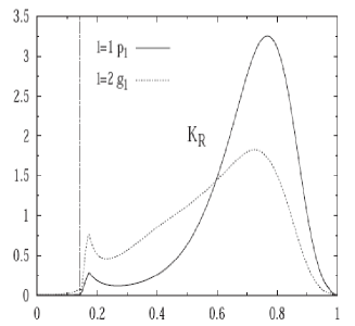
Figure 5: left: Schematic representation of the frequency spectrum of HD129929 (data from Aerts et al., 2004). right: Rotational kernels for the excited p1 and g1 modes of HD129929 in function of the radius $r/R$ normalized to the stellar radius (from Dupret et al., 2004).

Assuming therefore a uniform rotation for the convective core with angular velocity $\Omega=\Omega_{c}$ and a uniform rotation $\Omega=\Omega_{e}$ for the envelope of the star, the splittings then obey $S=\Omega_{c}\beta_{c}+\Omega_{e}\beta_{e}$ where $\beta_{j}$ are the integral for the core or the envelope (Sect.3.3). It is found that $|\beta_{c}|<<|\beta_{e}|$ that-is actually the detected modes do not efficiently probe the convective core. This can be seen with the associated rotational kernels in Fig.5 which have no amplitude in the core. Therefore $\Omega_{c}$ is taken as the rotation rate of the radiative region in the $\mu$-gradient region above the convective core (with $\mu$ the mean molecular weight). Assuming a linear depth variation of the angular velocity in the envelope $\Omega(x)=\Omega_{0}+(x-x_{0})\Omega_{1}$, the splittings must obey $S=\Omega_{0}\beta_{0}+\Omega_{1}\beta_{1}$ where again $\beta_{0}$ and $\beta_{1}$ are known from the stellar model;

$$\beta_{0}=\int_{0}^{x_{c}}K(x)~{}dx~{}~{};~{}~{}\beta_{e}=\int_{x_{c}}^{x_{e}}~{}K(x)(x-x_{c})~{}dx$$

The knowledge of $S_{1}$ and $S_{2}$ then yields $\Omega_{0}$ and $\Omega_{1}$. A rotation gradient in the envelope with $\Omega_{c}/\Omega_{e}=3.6$ is obtained.

In addition, the seismic modelling of the detected axisymmetric modes favors a core overshooting distance of $\sim 0.1$ pressure scale height ($H_{p}$) rather than 0 while an overshoot of $0.2\,H_{p}$ is rejected.

Figure 6: Schematic representation of the power spectrum of left: $\theta$ Ophiuchi (data from Handler et al., 2005) and right: $\nu$ Eri (data from Jerzykiewicz et al., 2005)

$\theta$ Ophiuchi

is also a main sequence $\sim 9\,M_{\odot}$ star with an effective temperature $T_{eff}\sim 22900~{}K$. Three multisite campains seismic observations and data analyses reveal 7 identified frequencies: the radial fundamental $\ell=0$ (p1); one triplet $\ell=1(p1)$ and 3 components $(m=-1,1,2)$ of a quintuplet $\ell=2$ (g1) (Handler et al., 2005). A seismic analysis led Briquet et al. (2007) to conclude that the case of $\theta$ Ophiuchi is similar to HD129929. The detected modes do not provide strong constraint about the rotation of the convective core. On the other hand, unlike HD129929, the data for $\theta$ Ophiuchi are compatible with a uniform or a quite slowly varying rotation of the envelope. The convective core overshoot distance is found to be $(0.44\pm 0.07)~{}H_{p}$ This is a much larger amount than found for HD129929. Whether this difference must be related to the fact that $\theta$ Ophiuchi seems to rotate more than 10 times faster than HD129929 remains an open issue.

$\nu$ Eri

is a very interesting case as it oscillates with 3 triplets $\ell=1$ ($g_{1}$, $p_{1}$, $p_{2}$), one radial mode $p_{1}$ and one $\ell=2$ component. Seismic studies show that the detected modes are able to probe the rotation of the core, which is rotating faster than the envelope (Pamyatnykh et al., 2004, PHD04; Ausseloos et al., 2004; Dziembowski & Pamyatnykh, 2008 (DP08); Suarez et al. 2009). DP08 further assumed a linear gradient as a transition (in the $\mu$ gradient zone) between the uniform fast rotation $\Omega=\Omega_{c}$ of the core and the uniform slow rotation of the envelope $\Omega=\Omega_{e}$ above the $\mu$-gradient region. They find a ratio $\Omega_{c}/\Omega_{e}=5.3-5.8$. Model fitting based on the 3 axisymmetric $\ell=1$ modes yield an extension of the mixed central region of 0.1-0.28 $H_{p}$ above the convective core radius depending on the adopted chemical mixture and metallicity value (DP08; Suarez et al., 2009).

Table 1: Overshoot versus rotation rate for several stars from seismic analysis. $Veq$ is the derived the equatorial velocity, $\alpha_{ov}$ the overshoot parameter, $\Omega_{inner}/\Omega_{env}$ the ratio of the the rotation rate in the inner layers to that of the surface, $Z$ the metallicity. The modellings assume a Grevesse-Noels mixture except for $12Lac$.

$\beta$ Cep	Veq (km/s)	$\alpha_{ov}$	$\Omega_{inner}/\Omega_{env}$	Z	ref
HD129929	$\sim$ 2	0.1 $\pm$ 0.05	$\Omega_{0.2}/\Omega_{surf}\sim 3.1$	0.019 $\pm$ 0.003	(1)
$\theta$ Ophiuchi	29 $\pm$ 7	$0.44^{*}\pm$ 0.07	env. unif. rotation	0.012 $\pm$0.003	(2)
$\nu$ Eri	$\sim$ 6	0.15 $\pm$ 0.05	$\Omega_{c}/\Omega_{env}\sim 5.5-5.8$	0.0172 $\pm$0.0013	(3)
$12Lac$	$\sim$ 49	$<0.4$	$\Omega_{c}/\Omega_{env}\sim 1.8-5$	0.01-0.015	(4), (5)
*Asplund mixture

(1) Dupret et al., 2004 (2) Briquet et al., 2007 (3) Pamyathnyck et al., 2004, (4) DP08 (5) Desmet et al., 2009

12 Lac

Several frequencies have been detected for this star (Handler et al., 2006) but only 4 of the detected frequencies correspond to identified $(\ell,m)$ modes (Desmet et al., 2009). Only 2 successive components of one $\ell=1$ triplet are known which is not enough to provide information on the inner/surface rotation ratio. One can use as an additional information the equatorial surface value, $v_{eq}=49\pm 3$ km/s as derived by Desmet et al. (2009). One needs the stellar radius which is derived from a seismic modelling of the star. The resulting seismic model and its radius depend on the radial orders identified for the modes (DP08 and Desmet et al., 2009). Second order (centrifugal) effects on the frequencies must also be taken into account as the rotation for 12 Lac seems to be fast enough as recognized by DP08. Taking then a value for the stellar radius in the broad range $R=7-9R_{\odot}$ , the equatorial surface value, $v_{eq}=49\pm 3$ km/s and the observed splitting of $1.3032\mu$Hz yields a ratio ${\Omega_{inner}/\Omega_{surf}}$ in the range $[1.8-5]$ definitely indicating a non rigid rotation. There is not yet an agreement concerning the radial order of the identified modes but the triplet seems in any case to be of mixed nature and therefore able to probe the core rotation. DP08 did not consider overshoot and Desmet et al. (2009) found that core overshoot must be smaller than 0.4 Hp.

Summary

These studies lead to the conclusion that a few rotationally split modes can provide important information about internal rotation and core overshoot of $\beta$ Cephei stars if the modes are identified, enough precise measurements are obtained and the age of the star is such that excited modes have mixed g, p nature. Trying to disentangle overshoot and rotation effects on core element mixing is only starting with a measure of their relative magnitude as is illustrated in Table 1. As emphasized by DP08, in that respect, seismic modelling of fast rotators are needed. Once the size of the mixed core and the ratio of core to surface rotation are reliably determined, the next issue is to estimate , what part in the seismically measured extension of the core, $d_{ov}$, comes from convective eddy overshooting and what part comes from other transport processes such as those induced by rotation.

4.2 Splitting asymmetries : distorsion

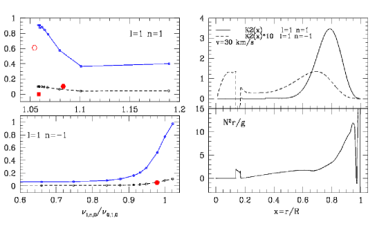
Figure 7: left: Scaled asymmetries ${\cal R}_{m}~{}10^{3}$ for $\ell=1$ $n=1$ (top) and $n=-1$ (bottom) modes in function of the $m=0$ frequency scaled by the radial fundamental mode frequency. The open dot (resp. full dot, full square) represents the observed asymmetry for $\theta$ Oph, (resp. for V386 Cen, $\nu$ Eri). The solid (resp. dashed) line corresponds to $v=30$ km/s (resp. 10 km/s) $8.2M_{\odot}$ models. The central hydrogen content $X_{c}$ is decreasing toward the right. top right: Kernels $K_{2}(x)$ for splitting asymmetries of $\ell=1,n=1$ (p1) mode (solid line) and $\ell=1,n=-1$ (g1) mode (dashed line) for model with $Xc=0.35$. The abscissae is the normalized radius.bottom right Run of the normalized Brünt-Väissälä profile $N^{2}r/g$ for the corresponding model with r/R. from Goupil & Talon, 2008)

The splitting asymmetry, $A_{m}$ (Eq.38), for acoustic modes is mainly due to the oblateness of the star caused by the centrifugal force although for low radial order modes, the Coriolis contribution is also significant. Fig.7 represents the normalized splitting asymmetries:

$${\cal R}_{m}\equiv A_{m}/\nu_{0,1,0}$$ (55)

for the $\ell=1,p_{1}$ and $g_{1}$ modes in function of the scaled frequency $y=\nu_{\ell,n,0}/\nu_{0,1,0}$ where $\nu_{0,1,0}$ is the frequency of the radial fundamental mode. ${\cal R}_{m}$ is plotted for $\theta$ Ophiuchi, HD129929 and $\nu$ Eri. The same quantities for 8.2 $M_{\odot}$ stellar models are also represented. The models have been computed with CESAM2k code (Morel, 1997) assuming standard physics (Lebreton et al., 2008; Goupil 2008) including a core overshooting distance of 0.1 $H_{p}$ and an initial hydrogen abundance $X=0.71$ and metal abundance $Z=0.014$. The evolution of the selected models is represented by the central hydrogen content $X_{c}$ from 0.5 to 0.2. The frequencies have been computed using a second order perturbation method and an adiabatic oscillation code WAR(saw)M(eudon) adapted from the Warsaw’s oscillation code (Daszyńska-Daszkiewicz et al., 2002). For each model, two sets of frequencies are computed assuming a uniform rotation corresponding to $v=30$ km/s and $v=10$ km/s respectively. These sequences of models do not represent true evolutionary sequences as in realistic conditions, the rotation changes with time and can be non uniform. They however illustrate the evolution of the asymmetry when a mode changes its nature during evolution, from pure p mode to mixed p and g mode for instance. Indeed pure g modes have small asymmetries compared with pure p modes because they have much smaller amplitude in the outer envelope where distorsion has its most significant effect. This is illustrated in Fig.7. In a perturbation description, one finds that ${\cal R}_{m}$ is a second order effect proportional to $\Omega^{2}$ (DG92; Goupil et al., 2000; Goupil, 2009 and references therein). The variation of ${\cal R}_{m}$ with the scaled frequency $y$ (ie with stellar evolution) is similar for the $v=30$ and $v=10$ km/s sequences of models but ${\cal R}_{m}$ is roughly 9 times (ie ratio of $\Omega^{2}$) larger for $v=30$ km/s models than $v=10$ km/s models. For pure p modes, the asymmetry amounts to ${\cal R}_{m}\sim 0.8~{}10^{-3}$ whereas for pure g modes it almost vanishes. ${\cal R}_{m}$ for the $\ell=1,n=1$ mode decreases for older models (larger y). The reverse happens for the $\ell=1,n=-1$ mode. The reason is that for young models, $\ell=1,n=1$ and $n=-1$ modes are pure p and g modes respectively. When the model is more evolved, these 2 modes experience an avoided crossing and exchange their nature. From a perturbative approach, one derives:

$$A_{m}=\nu_{\ell,n,0}~{}\int_{0}^{1}\hat{\Omega}^{2}(x)~{}K_{2}(x)~{}dx$$ (56)

where $\hat{\Omega}^{2}=\Omega^{2}/(GM/R^{3})$ and $x=r/R$ the radius normalized to the surface radius. $K_{2}(x)$ depends on the centrifugal perturbation part of pressure and density as well as the differential rotation $\Omega(x)$ and the mode eigenfunction. Fig.7 shows $K_{2}(x)$ in function of the normalized radius $x=r/R$ for $\ell=1,n=1~{}(p_{1})$ and $\ell=1,n=-1~{}(g_{1})$ modes for the $v=30$ km/s, 8.2 $M_{\odot}$ model with $X_{c}=0.5$. The inner layers contribute to the asymmetry of $\ell=1,g_{1}$ multiplet in contrast with the $\ell=1,p_{1}$ multiplet for which the kernel $K_{2}$ is concentrated toward the surface layers. The asymmetry of the $\ell=1,g_{1}$ multiplet is sensitive to the inner maximum of the Brünt-Väissälä frequency, arising from the $\mu$-gradient, which contributes negatively to $K_{2}$. As the negative contribution is very localized, it decreases the asymmetry only slightly compared to a pure p mode for a uniform rotation. However, one can expect a larger decrease in case of a rotation faster in the inner regions than the surface.

Theoretical estimates seem to disagree with observed asymmetries deduced from $\ell=2$ modes for $\theta$ Ophiuchi (Briquet et al., 2007) and $\nu$ Eridani for $\ell=1,p_{2}$ (Dziembowski & Jerzykiewicz, 1999, PHD04, Suarez et al. 2009). Is the disagreement real? The question has some relevance as the asymmetry values are only marginally above the observation uncertainties. Or can it be that the observed frequencies do not belong to the same multiplet as suggested by DP08 for $\nu$ Eri?

4.3 Axisymmetric modes: mixing

Rotationally induced mixing of chemical elements changes the structure and in particular affects the Brünt-Väissälä frequency $N$ at the border of the convective core. As a consequence, at a given location in a HR diagram corresponding to an observed star, one can find several models with different structures and therefore likely different values of the mode frequencies including axisymmetric modes which can then be used as diagnostics for mixing.

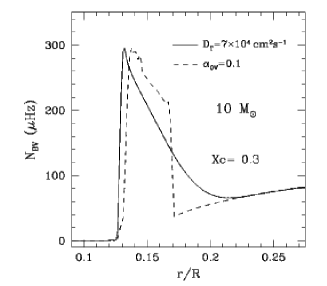
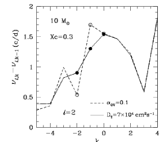
Figure 8: left: Brünt-Väissälä profile in the central region of a 10 $M_{\odot}$ model with $X_{c}=0.3$ and an initial velocity of 50 km/s. right: the large separation $\nu_{\ell,n,0}-\nu_{\ell,n-1,0}$ in function of the radial order n for $\ell=2$ modes for a model including turbulent mixing (solid) line and a model including a $0.1~{}H_{p}$ overshoot instead (dashed line). (from Montalban et al. 2008)

Uniform and constant diffusion coefficient $D_{t}$:

Montalban et al. (2008) and Miglio et al. (2008) investigated the effect of turbulent mixing on a g-mode frequency spectrum and the ability of such modes to probe the size of stellar convective cores. They assumed a constant in time and uniform in space global diffusion coefficient $D_{t}=D_{eff}+D_{v}$ in Eq. 1 above. The constant value for $D_{t}$ is chosen so as to correspond to the value near the convective core provided by a Geneva stellar model including rotationally induced mixing. This is valid for g-modes which have most of their amplitude there (see Miglio et al., 2008) The model is a mid main sequence ($X_{c}=0.3$) 10 $M_{\odot}$ with $D_{t}=7~{}10^{4}$ cm²/s chosen to correspond to a rotational velocity $v$= 50 km/s.

Fig.8 shows the Brünt-Väissälä frequency ($N$) profile for a model with turbulent chemical element mixing and a model with no turbulent chemical element mixing but including instead core overshoot assuming an overshoot distance of 0.1 $H_{p}$. Differences can be seen at the edge of the convective core. The Brünt-Väissälä frequency of the model with turbulent mixing behaves more smoothly in the $\mu$-gradient region above the convective core than for the model computed with no turbulent mixing but with an overshoot distance of $0.1\,H_{p}$. From Geneva code calculations, the evolution of the rotation profile leads to a core to envelope ratio of 1.6. The differences between the two profiles arising at the edge of the convective core cause significant changes on frequencies of g-modes and mixed modes. The frequency separations $\Delta_{n,\ell}=\nu_{\ell,n,0}-\nu_{\ell,n-1,0}$ differ by a few $\mu$Hz for radial order $n=-1$ and $n=-2$ , $\ell=2$ modes between the model with overshoot $0.1\,H_{p}$ and the model with turbulent mixing (Fig.8). At higher frequencies for pure p-modes, no differences in $\Delta_{n,\ell}$ are seen when adding turbulent mixing or not.

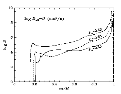
Figure 9: Run of the rotationally induced turbulent coefficient, $D_{t}$, with the relative shell mass at 3 different evolutionary stages with ages 0.5 Myr, 1 Myr and 1.5 Myr respectively and labelled with their central hydrogen content $X_{c}$- leading to the stellar model $V_{15}$ ($X_{c}=0.3$) (from Goupil & Talon 2008).

Rotationally induced diffusion coefficient

In this section, we consider stellar models which are computed with the Toulouse-Geneva evolutionary code which includes the coupling between rotationally induced mixing and momentum transport (Eq.1 and Eq.2 above) as described by Talon (2008). The rotational evolution of the star begins from solid body when the core is still radiative, shortly after the star leaves the Hayashi track. A $8.5\,M_{\odot}$ mass has been chosen so that the models evolve through the HR diagram to a location where the star $\theta$ Ophiuchi is expected ($\log L/L_{\odot}=3.73$, $T_{\rm eff}=4.35$). This corresponds to a mid main sequence model, $V_{15}$, with a central hydrogen content $X_{c}=0.3$. The evolution has been initiated with a uniform rotational velocity $v=15$ km/s on the pms; the rotation profile then evolves to strongly differential rotation so that $V_{15}$ has a surface velocity of $v=48.2$ km/s and a ratio $\Omega_{core}/\Omega_{surf}=1.6$ when crossing the $\theta$ Ophiuchi location in the HR diagram at an age of 19.65 Myr.

Figure 10: Model $V_{15}$ with a surface rotational velocity v=48.2 km/s. top: Profile of of the normalized Brünt-Väissälä frequency as defined by $N^{2}~{}r/g$ in function of the normalized radius $r/R$. Bottom: rotation profile normalized to its surface value. The core to surface ratio for the rotation rate then is 1.6 (from Goupil & Talon 2009 in prep.).

The diffusion coefficient, $D_{t}$, depends on the meridional circulation velocity and the local turbulence strength. It varies with depth and evolves with time as illustrated in Fig.9. The $D_{t}$ profile is represented for 3 models with ages 0.5 Myr, 1 Myr and 1.5 Myr built assuming an initial 15 km/s velocity on the pms. The rotation evolving from uniform to strongly differential rotation causes a relaxation toward a stationary profile which persists with only an ajustement due to expansion and contraction with evolution (Goupil & Talon 2008).
Effect of rotationally induced mixing on the structure is significant at the edge of the convective core as emphasized in Fig.9 where we compare the squared Brünt-Väissälä profile, $N^{2}$, in the vicinity of the edge of convective core for model $V_{15}$ and a model $V_{0}$ which includes neither rotationally induced mixing nor overshoot. Inclusion of rotationally induced mixing leads to the model ${\bf V_{15}}$ which shows a narrower maximum of Brünt-Väissälä profile at the edge of the convective core compared with that of ${\bf V_{0}}$.

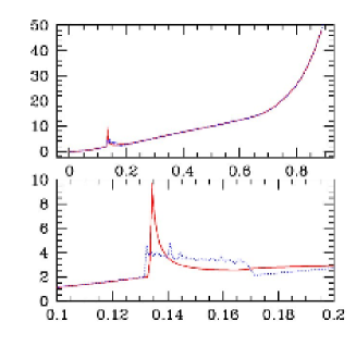
Figure 11: left top: Zoom of Brünt-Väissälä frequency profile in the vicinity of the edge of convective core in function of the normalized radius $r/R$ for model $V_{15}$ (dashed line) and model $V_{0}$ (solid line). The local maximum of $N^{2}r/g$ corresponds to a nonzero $\mu$-gradient. It decreases more sharply in presence of rotationally induced mixing because mixing results in smoothing the $\mu$-gradient. Left bottom: Differences $\delta\nu=\delta\omega/(2\pi)$ between frequencies computed from model $V_{0}$ (no rotationally induced mixing included) and model $V_{15}$ for $\ell=0$ (solid line) and $\ell=1$ (dashed line) $m=0$ modes in $\mu$Hz (from Goupil & Talon, 2008). right: $d\ln\rho/d\ln r$ in function of the normalized radius $r$ for model $V_{15}$ (dashed line)and model $V_{0}$ (solid line) right top: from center to surface, right bottom: in the central region (from Goupil & Talon 2009, in prep.)

To illustrate the impact of such a difference on the oscillation frequencies, we compare low radial order frequencies of the models ${\bf V_{15}}$, and ${\bf V_{0}}$. Modes $p_{1}$, $p_{2}$, $g_{1}$ for these models have amplitudes near the edge of the convective core. Fig.11 shows that this can result in significant frequency differences for the same mode easily detectable with CoRoT observations. The frequencies of these modes are quite sensitive to the detail of the Brünt-Väissälä profile in this region. This means that some care must be taken when computing these frequencies and drawing conclusions. The frequencies of these modes are indeed sensitive not only to the physics but unfortunately also to the numerics which can be quite inaccurate in this region of the star.

The sign and magnitude of $\delta\omega=\omega_{V15}-\omega_{V0}$ are dependent on the mode when it has amplitude in the regions where the nonrotating model and the model with rotationally induced mixing differ. We consider here, as in Sec.3.5, only the effect of rotationnally induced mixing on the spherically symmetric structure. Differences in the structure of the model $V_{15}$ which includes rotationnaly induced mixing and the model $V_{0}$ which does not result in differences in the eigenfrequencies which we note $\delta\omega=\omega_{0,\Omega}-\omega_{0,\Omega=0}$.

The structure of the models $V_{15}$ and $V_{0}$ indicates that $p_{\Omega}$ and its derivative, the gravity $g_{\Omega}$, the density $\rho_{\Omega}$ are not significantly modified compared to the derivative of the density. Fig.11 shows that the largest difference $\delta({d\log\rho_{\Omega}/d\log r})$ arises near the convective core. Accordingly from Eq.54, one expect larger frequency differences $\delta\omega$ for mixed modes compared to p-modes. This is what is observed in Fig.11. As explained in Sect.3.5, with the help of the integral relation for $\delta\omega$, the frequency differences for high frequency (i.e. pure) p-mode is small and positive. For lower frequency mixed modes, $\delta\Bigl{(}{d\ln\rho_{\Omega}\over d\ln r}\Bigr{)}$ can be positive and the frequency difference can be large and negative as illustrated in Fig.11.

5 Cubic order versus latitudinal dependence

It has been known for a long time that latitudinal variations of the rotation rate generate departures from linear splitting. On the other hand, a fast uniform rotation can generate cubic order corrections to the frequency of non axisymmetric modes which also cause departure from linear splitting. The latitudinal correction to the linear splitting is proportional to the $\Omega$ gradient whereas cubic order effects, as their name indicate, are proportional to $\Omega^{3}$. It is expected that the dependence of these corrections with the frequency differs when it is due to latitudinal differential rotation or to cubic effects.

Low mass stars are known to be slow rotators. Indeed due to their outer convection zone, they undergo magnetic braking. Due again to their outer convection zone, obervational evidences exist for surface latitudinal differential rotation. Hence for these stars, the averaged rotation rate $\Omega$ is small and $\Delta\Omega=\Omega_{equa}-\Omega_{pole}$, the difference between the rotation rates at the equator and the poles, can be large (25% -30% for the Sun, between 1% and 45% for a star like Procyon, Bonanno et al. 2007). One therefore expects that latitudinal corrections to the splittings dominate over cubic order ones which are negligible. On the other hand, more massive stars on the main sequence have shallower convection zones which even disappear above $\sim$ 3- 5 $M_{\odot}$. These stars usually are fast rotators with a radiative envelope which may or may not be in latitudinal differential rotation. For these fast rotators, one can wonder what is the minimal latitudinal shear which dominates over cubic order effects and can therefore be detectable. Here we quantify this issue with the help of a polytropic model with index 3. The constants characterizing the polytrope are taken to correspond to model A considered in Sect.4.3. We establish first the splitting correction due to latitudinal differential rotation. This is then compared with the splitting correction arising from cubic order effects as derived by previous works. We assume a rotation velocity of 100 km/s.

5.1 Latitudinal dependence

Hansen et al. (1977) derived the expression for the rotational splitting of adiabatic nonradial oscillations for slow differential (steady, axially symmetric) rotation $\Omega(r,\theta)$ and applied it to numerical models of white dwarfs and of massive main sequence stars assuming a cylindrically symmetric rotation law. In the solar case, the effects of latitudinal differential rotation on theoretical frequencies were investigated by Gough & Thompson (1990), Dziembowski & Goode (1991, DG91) and DG92 who also considered the case of $\delta$ Scuti stars.

In order to be able to compute the splittings from Eq.17 and Eq.24, one must specify a rotation law. It is convenient to assume a rotation of the type:

$$\Omega(r,\theta)=\sum_{s=0}^{s_{max}}~{}\Omega_{2s}(r)~{}(\cos\theta)^{2s}$$ (57)

where $\theta$ is the colatitude and we take $s_{max}=2$. The surface rotation at the equator is $\Omega(r=R,\theta=\pi/2)=\Omega_{0}(r=R)$. Note that in the solar case, $\Omega_{2}$, $\Omega_{4}$ are negative and the equator rotates faster than the poles (DG91, Schou et al., 1998). As shown in Appendix, inserting Eq.57 into Eq.24 yields the following expression for the generalized splitting (Eq.108 in Appendix):

$$S_{m} = \int_{0}^{R}\Omega_{0}(r)~{}K(r)~{}dr+\sum_{s=0}^{s=2}m^{2s}~{}H_{s}(\Omega)$$ (58)

with $K(r)$ defined in Eq.27 and

$$H_{s}(\Omega)=$$ (59)

$$- {1\over I}\int_{0}^{R}~{}\Omega_{0}(r)~{}\Bigl{[}R_{s}~{}\Bigl{(}\xi^{2}_{r}-2\xi_{r}\xi_{h}+\xi^{2}_{h}(\Lambda-1)\Bigr{)}+Q_{s}~{}\xi^{2}_{h}\Bigr{)}\Bigr{]}\rho_{0}r^{2}dr$$ (60)

where $R_{s}$ and $Q_{s}$ depend on $\Omega_{2},\Omega_{4}$ and $\Lambda=\ell(\ell+1)$ and are given by Eq.103 and Eq.107 (Appendix) respectively.

a) Uniform rotation In that case, $\Omega(r,\theta)=\Omega_{0},~{}\forall r$, $\theta$; $\Omega_{2},\Omega_{4}=0$ i.e. $R_{j},Q_{j}=0$ for $j=0,2$ hence $H_{m,j}=0$. One recovers the well known expression:

$$S_{m} = \Omega_{0}~{}\beta$$ (61)

where, for later purpose, we have defined

$$\beta = \int_{0}^{R}~{}K(r)~{}dr$$ (62)

$$= -{1\over I}\int_{0}^{R}~{}\Bigl{[}\Bigr{.}\xi_{r}^{2}-2\xi_{r}\xi_{h}+(\Lambda-1)~{}\xi_{h}^{2}\Bigl{.}\Bigr{]}~{}\rho_{0}r^{2}dr$$ (63)

This is usually rewritten as :

$$S_{m}=\Omega_{0}~{}(C_{L}-1)$$

where $C_{L}$ is the Ledoux (1951) constant

$$C_{L}={1\over I}\int_{0}^{R}~{}\Bigl{[}2\xi_{r}\xi_{h}+\xi_{h}^{2}\Bigr{]}~{}\rho_{0}r^{2}dr$$

b) Shellular rotation then $\Omega(r,\theta)=\Omega_{0}(r)$ and $s_{max}=0$; again here: $\Omega_{2},\Omega_{4}=0$ ie $R_{j}=Q_{j}=0$ for $j=0,2$ and

$$S_{m} = -{1\over I}\int_{0}^{R}~{}\Omega_{0}(r)~{}\Bigl{[}\Bigr{.}\xi_{r}^{2}-2\xi_{r}\xi_{h}+\Lambda~{}\xi_{h}^{2}\Bigl{.}\Bigr{]}~{}\rho_{0}r^{2}dr$$ (64)

c) Latitudinally differential rotation only In that case, $\Omega_{2j},j=0,2$ are depth independent and $R_{s}$ and $Q_{s}$ are constant and

$$S_{m}=\Omega_{0}~{}\beta+\Omega_{0}~{}\sum_{s=0}^{s=2}m^{2s}~{}(R_{s}(\Omega)~{}\beta+Q_{s}(\Omega)~{}\gamma)$$ (65)

with $\beta$ defined in Eq.63 and

$$\gamma=-{1\over I}\int_{0}^{R}~{}\xi^{2}_{h}~{}\rho_{0}r^{2}~{}dr$$

For a triplet $\ell=1$, $m=1$ ($\Lambda=2$) then

$$S_{1} = \Omega_{0}~{}\beta+\Omega_{0}~{}(R(\Omega)~{}\beta+Q(\Omega)~{}\gamma)$$ (66)

with (using Eq.103 and Eq.107):

$$R(\Omega) = \sum_{s=0}^{s=2}~{}R_{s}(\Omega)={1\over 5}{\Omega_{2}\over\Omega_{0}}+{3\over 7}~{}{\Omega_{4}\over\Omega_{0}}$$ (67)

$$Q(\Omega) = \sum_{s=0}^{s=2}~{}Q_{s}(\Omega)=-{24\over 5}{\Omega_{4}\over\Omega_{0}}$$ (68)

In the solar case, $\beta\sim-1$ and $|\beta|>>|\gamma|$ for the excited high frequency p-modes.

$$S_{1} \approx -\Omega_{0}~{}\Bigl{(}1+{1\over 5}{\Omega_{2}\over\Omega_{0}}+{3\over 7}~{}{\Omega_{4}\over\Omega_{0}}\Bigr{)}$$ (69)

With $\Omega_{2}/\Omega_{0}=-0.127,\Omega_{4}/\Omega_{0}=-0.159$ (from DG89), one obtains a departure from linear splitting of $|{S_{1}/\Omega_{0}}+1|=0.093$ i.e. a $\approx$ 10% change in the solar case. For upper main sequence stars, excited modes are around the fundamental radial mode and may be mixed modes with $|\beta|\sim|\gamma|\sim 1/2$. This leads for instance to $|{S_{1}/\Omega_{0}}+1/2|\approx 5\%$ for $\Omega_{2}/\Omega_{0}$ and $\Omega_{4}/\Omega_{0}$ equal to 1/5 of the solar values.

5.2 Latitudinal dependence versus cubic order effects

Let assume on one side a pulsating star uniformaly rotating with a rate $\Omega_{0}$ high enough that cubic order ($O(\Omega_{0}^{3})$) contributions are significant. On the other side, one also considers a model rotating with a latitudinally differential rotation (uniform in radius). One issue then is which one of these two effects dominate over the other one since the cubic one is $O(\Omega^{3})$ whereas the other one is $O(\Delta\Omega)$ ? For stars other than the Sun, one can simply assume the rotational latitudinal shear $\Delta\Omega=\Omega_{2}$ with $\Omega_{4}=0$ and $\Omega(\theta)=\Omega_{0}+\Delta\Omega\cos^{2}\theta$. For $\ell=1$ modes, Eq.66 becomes

$$S_{1}(lat)=\Omega_{0}~{}\beta\Bigl{(}1+{1\over 5}{\Delta\Omega\over\Omega_{0}}\Bigr{)}$$ (70)

Expressions for the frequency correction (in rad/s) for cubic order effects assuming a uniform rotation has been derived by Soufi et al. (1998). Part of the cubic order effet is included in the eigenfrequency $\omega_{0,\Omega}$ and therefore is also included in second order coefficients which indeed involve $\omega_{0,\Omega}$. Another part of the cubic order effects is included as an additive correction to the frequency.

Frequency up to 3rd order were computed for models of $\delta$ Scuti stars by Goupil et al. (2001), Goupil & Talon (2002), Pamyatnykh (2003), Goupil et al. (2004). Karami (2008) rederived the cubic order effects following Soufi et al.’s approach and Karami (2008, 2009) applied it to a ZAMS model of a 12 $M_{\odot}$ $\beta$ Cephei star. He found that cubic order effects are of the order of $0.01\%$ for a $l=2,n=2$ and $0.5\%$ for a n=14 mode for a 100 km/s rotational velocity. Values of the third order additive correction to the frequency were listed for $\ell=1$ p-modes of a polytrope of index 3 by Goupil (2009).

Here we write the splitting under the form:

$$S_{m}(cubic)=\Omega_{0}~{}\beta+\Omega_{0}~{}\Bigl{(}{\hat{\Omega}_{0}\over\sigma_{0}}\Bigr{)}^{2}~{}T_{|m|}$$ (71)

where the last term represents the full cubic order contribution with $\sigma_{0}$ is the normalized frequency of the nonrotating polytrope and $\hat{\Omega}_{0}=\Omega_{0}/\Omega_{K}$.

Tab.2 lists the value of the dimensionless coefficients $T_{1}/\sigma^{2}_{0}$ and $-\beta,-\gamma$ for $\ell=1$ modes for a polytrope with a polytropic index 3. The coefficient ${T_{1}/\sigma^{2}_{0}}$ remains nearly constant with increasing frequency for frequencies above $\sigma_{0}>10$ i.e. for p modes For $\sigma_{0}>10$ (p-modes), $-\beta\approx 1$ and $T_{1}/\sigma^{2}_{0}\approx-0.09$. The splitting is decreased by a latitudinal dependence with $\Delta\Omega<0$ whereas it is increased by cubic order effects $T_{1}/\beta>0$ . In absolute values, the effect of latitudinal differential rotation on the splittings then dominates over cubic order effects whenever:

$$|{\Delta\Omega\over\Omega_{0}}|>0.45~{}\hat{\Omega}^{2}_{0}$$

For model A and a rotational velocity 100 km/s, $\hat{\Omega}_{0}=0.174$ then $|{\Delta\Omega\over\Omega_{0}}|>1.36\%$ For a faster rotator with for instance 200 km/s,the latitutinal shear must be larger i.e. $|{\Delta\Omega\over\Omega_{0}}|>~{}5.45\%$.

For the slowly rotating $\beta$ Cep stars considered in Sect.4 above ($v<50$ km/s), cubic order effects in the splittings can be neglected in front of latitudinal effects equal or larger than $0.34\%$. At this low level, both effects are comparable to the observational uncertainties ($0.1\%$).

Table 2: Coefficients assuming a uniform rotation for a polytrope with polytropic index $3$ and adiabatic index $\gamma=5/3$. The squared frequency $\sigma^{2}_{0}$ is the dimensionless squared frequency $\omega^{2}/(GM/R^{3})$. Spherical centrifugal distorsion of the polytrope has not been included.

				$\ell=1$
n	$\sigma^{2}_{0}$	$C_{L0}$	$X_{1}$	$X_{2}$	$Y_{1}$	$Y_{2}$	$T_{1}/\sigma^{2}_{0}$	-$\beta$	-$\gamma$
-7	0.22	0.479	0.417	0.008	0.012	-0.018	0.592	0.521	0.456
-6	0.28	0.476	0.419	0.005	0.015	-0.023	0.462	0.524	0.450
-5	0.37	0.473	0.422	0.001	0.020	-0.029	0.351	0.527	0.441
-4	0.52	0.469	0.425	-0.004	0.026	-0.039	0.254	0.531	0.431
-3	0.78	0.466	0.427	-0.013	0.038	-0.056	0.164	0.534	0.410
-2	1.28	0.466	0.428	-0.024	0.059	-0.089	0.073	0.535	0.386
-1	2.51	0.473	0.422	-0.035	0.106	-0.159	-0.025	0.528	0.269
1	11.37	0.029	0.777	0.877	2.890	-4.335	0.024	0.970	0.025
2	21.49	0.034	0.773	0.864	5.802	-8.703	-0.034	0.966	0.028
3	34.83	0.033	0.773	0.851	9.624	-14.436	-0.063	0.966	0.027
4	51.39	0.031	0.776	0.840	14.340	-21.511	-0.077	0.969	0.026
5	71.15	0.027	0.778	0.832	19.940	-29.909	-0.084	0.973	0.025
6	94.09	0.024	0.781	0.826	26.414	-39.621	-0.088	0.976	0.023
7	120.19	0.021	0.783	0.821	33.757	-50.635	-0.089	0.979	0.022
8	149.43	0.019	0.785	0.817	41.964	-62.946	-0.089	0.981	0.020
9	181.81	0.017	0.787	0.814	51.032	-76.548	-0.089	0.984	0.019
10	217.32	0.015	0.788	0.811	60.958	-91.437	-0.089	0.985	0.018
11	255.94	0.013	0.789	0.809	71.739	-107.609	-0.088	0.987	0.017
12	297.67	0.012	0.790	0.807	83.375	-125.062	-0.087	0.988	0.017
13	342.51	0.011	0.791	0.805	95.862	-143.793	-0.087	0.989	0.016
14	390.44	0.010	0.792	0.804	109.201	-163.802	-0.086	0.990	0.015
15	441.47	0.009	0.793	0.803	123.392	-185.087	-0.085	0.991	0.014
16	495.59	0.008	0.793	0.802	138.432	-207.648	-0.085	0.992	0.014
17	552.80	0.008	0.794	0.801	154.323	-231.484	-0.084	0.993	0.013
18	613.09	0.007	0.794	0.800	171.064	-256.595	-0.084	0.993	0.013
19	676.47	0.006	0.795	0.799	188.655	-282.982	-0.083	0.994	0.012
20	742.93	0.006	0.795	0.798	207.097	-310.645	-0.083	0.994	0.012
21	812.46	0.006	0.796	0.798	226.389	-339.584	-0.082	0.995	0.012
22	885.08	0.005	0.796	0.797	246.534	-369.800	-0.082	0.995	0.011
23	960.78	0.005	0.796	0.797	267.530	-401.295	-0.082	0.995	0.011

6 Conclusions

We have seen along this review that several efficient seismic tools can be designed to obtain valuable information on the internal structure and dynamics of main sequence massive stars which oscillate with a few identified modes. Identification of the detected modes requires a high signal to noise which is made available due to the large amplitudes of these opacity-driven modes. On the other hand, these stars oscillate with low frequencies lying near/in the dense part of the spectrum where p modes, mixed modes and g modes can be encountered. While this is a great advantage in order to probe the inner layers of the star, resolution and precise measurement of quite close frequencies in a Fourier spectrum requires very long time series. This explains the yet still small number of $\beta$ Cephei stars for which a successful seismic analysis has been obtained, despite the appealing prospects that a better knowledge of their structure bring up valuable constrains on their still poorly understood life end as supernovae. It is expected that the space experiments CoRoT (Michel et al. 2008) and Kepler (Christensen-Dalsgaard et al., 2008) will increase the number of O-B stars for which fruitful seismic analyses can be carried out as well as possibly enlarge the sample to fast rotators. Mode identification can be at first difficult to perform for fast rotators but some of these fast rotating stars might also show oscillations of solar-like type which characteristics could help the mode identification. This interesting perspective has recently emerged with the discovery of the first chimera star with the CoRoT mission (Belkacem et al., 2009).

Appendix : Differential rotation

The expression for the mode splitting of adiabatic nonradial oscillations due to a differential rotation $\Omega(r,\theta)$ can be put into the compact form (Hansen et al. (1977), DG91, DG92, Schou et al. (1994a,b), Pijpers (1997), CD03):

$$\delta\omega_{m}=m~{}\int_{0}^{R}\int_{0}^{\pi}{\cal K}_{m}(r,\theta)~{}\Omega(r,\theta)~{}d\theta dr$$ (72)

where ${\cal K}_{m}$ is called rotational kernel:

$${\cal K}_{m}(r,\theta) = -{~{}\rho_{0}r^{2}\over I}{\sin\theta\over 2}~{}\Omega(r,\theta)\times$$ (74)

$$\int{d\phi\over 2\pi}~{}\Bigl{[}\Bigr{.}\Bigl{(}|\xi_{r}|^{2}-(\xi^{*}_{r}\xi_{h}+cc)\Bigr{)}~{}|Y_{\ell}^{m}|^{2}$$

$$+ |\xi_{h}|^{2}\Bigl{(}\nabla_{H}Y_{\ell}^{m*}\cdot\nabla_{H}Y_{\ell}^{m}-{\partial|Y_{\ell}^{m}|^{2}\over\partial\theta}{\cos\theta\over\sin\theta}\Bigr{)}\Bigl{.}\Bigr{]}$$ (75)

where the spherical harmonics $Y_{\ell}^{m}$ are normalized such that

$$\int(Y_{\ell}^{m^{\prime}})^{*}(\theta,\phi)~{}Y_{\ell}^{m}(\theta,\phi)~{}{d\Omega\over 4\pi}=\delta_{\ell,\ell^{\prime}}\delta_{m,m^{\prime}}$$

where $d\Omega=\sin\theta d\theta d\phi$ is the solid angle elemental variation and $\delta_{\ell,\ell^{\prime}}$ is the Kroenecker symbol. Mode inertia $I$ is given by

$$I=\int_{0}^{R}\Bigl{(}|\xi_{r}|^{2}+\Lambda~{}|\xi_{h}|^{2}\Bigr{)}~{}\rho_{0}r^{2}dr$$ (76)

with $\Lambda=\ell(\ell+1)$.

It is convenient to assume a rotation of the type:

$$\Omega(r,\theta)=\sum_{s=0}^{s_{max}}~{}\Omega_{2s}(r)~{}(\cos\theta)^{2s}$$ (77)

where $\theta$ is the colatitude. Eq.72 becomes:

$$\delta\omega_{m} = -{m\over I}\sum_{s=0}^{s_{max}}~{}\int_{0}^{R}~{}\Omega_{2s}(r)~{}~{}\times$$ (79)

$$\Bigl{[}\Bigr{.}~{}\Bigl{(}|\xi_{r}|^{2}-(\xi^{*}_{r}\xi_{h}+cc)\Bigr{)}~{}{\cal S}_{s}+|\xi_{h}|^{2}(B_{1}+B_{2})\Bigl{.}\Bigr{]}~{}\rho_{0}r^{2}dr$$

where we have defined

$${\cal S}_{s}\equiv\int~{}|Y_{\ell}^{m}|^{2}~{}(\cos\theta)^{2s}~{}{d\Omega\over 4\pi}=\int_{0}^{1}\mu^{2s}~{}|Y_{\ell}^{m}(\theta,\phi)|^{2}d\mu$$ (80)

with $\mu=\cos\theta$ and

$$B_{1} = \int~{}\Bigl{(}\nabla_{H}Y_{\ell}^{m*}\cdot\nabla_{H}Y_{\ell}^{m}\Bigr{)}(\cos\theta)^{2s}~{}{d\Omega\over 4\pi}$$ (81)

$$B_{2} = -\int~{}({\partial|Y_{\ell}^{m}|^{2}\over\partial\theta}{\cos\theta\over\sin\theta}\Bigr{)}~{}(\cos\theta)^{2s}~{}{d\Omega\over 4\pi}$$ (82)

The term in $|\xi_{h}|^{2}$ requires a little care. Consider first $B1$. Integration by part leads to

$$B1 = -\int{d\Omega\over 4\pi}~{}Y_{\ell}^{m*}~{}$$ (83)

$$\Bigl{[}\Bigl{(}\nabla^{2}_{H}Y_{\ell}^{m}\Bigr{)}~{}(\cos\theta)^{2s}+(\nabla_{H}Y_{\ell}^{m}\Bigr{)}~{}\cdot~{}\nabla_{H}((\cos\theta)^{2s})\Bigr{]}$$ (84)

Recalling that $\nabla^{2}_{H}Y_{\ell}^{m}=-\Lambda~{}Y_{\ell}^{m}$, one gets

$$B1 = \Lambda~{}{\cal S}_{s}-{1\over 2}\int~{}~{}\Bigl{[}Y_{\ell}^{m*}~{}{\partial Y_{\ell}^{m}\over\partial\theta}~{}{d(\cos\theta)^{2s})\over d\theta}+cc\Bigr{]}~{}{d\Omega\over 4\pi}$$ (85)

where cc means complexe conjugate. Again an integration by part yields

$$B1 = \Lambda~{}{\cal S}_{s}+{1\over 2}\int|Y_{\ell}^{m}|^{2}~{}{d\over d\theta}\Bigl{[}\sin\theta~{}{d(\cos\theta)^{2s})\over d\theta}\Bigr{]}~{}{d\theta\over 2}$$ (86)

One finally obtains

$$B1 = \Lambda~{}{\cal S}_{s}+s\Bigl{[}(2s-1){\cal S}_{s-1}-(2s+1){\cal S}_{s}\Bigr{]}$$ (87)

Turning to the second term $B_{2}$ in Eq.79, an integration by part yields

$$B_{2}=-(2s+1)~{}{\cal S}_{s}$$ (88)

Inserting expressions Eq.87 and 88 into Eq. 79, one obtains

$$\delta\omega_{m} = m~{}\sum_{s=0}^{s_{max}}~{}\int_{0}^{R}~{}\Omega_{2s}(r)~{}K_{m,s}(r)dr$$ (89)

with

$$K_{m,s}(r) = K(r)~{}{\cal S}_{s}-{1\over I}~{}\rho_{0}r^{2}~{}|\xi_{h}|^{2}s~{}\Bigl{[}(2s-1){\cal S}_{s-1}-(2s+3){\cal S}_{s}\Bigr{]}$$ (90)

and

$$K(r)=-{1\over I}~{}\Bigl{[}|\xi_{r}|^{2}-(\xi^{*}_{r}\xi_{h}+cc)+|\xi_{h}|^{2}(\Lambda-1)\Bigr{]}~{}\rho_{0}~{}r^{2}$$ (91)

Expression Eq.90 is equivalent to Eq.25 in DG92. For any $s$, ${\cal S}_{s}$ is given by a recurrent relation (Eq.31 in DG92). Note that $\delta\omega_{m}=\delta\omega_{-m}$. Let define the generalized splitting

$$S_{m}={\omega_{m}-\omega_{-m}\over 2m}={\delta\omega_{m}-\delta\omega_{-m}\over 2m}={\delta\omega_{m}\over m}$$

We limit the expression for the rotation to $s_{max}=2$ i.e.:

$$\Omega(r,\theta)=\Omega_{0}(r)+\Omega_{2}(r)~{}\cos^{2}\theta+\Omega_{4}(r)~{}\cos^{4}\theta$$ (92)

then for adiabatic oscillations ($\xi_{r}(r)$ and $\xi_{h}(r)$ are real):

$$K_{m,0}(r) = K(r)$$ (93)

$$K_{m,1}(r) = K(r)~{}{\cal S}_{1}-{1\over I}~{}\xi^{2}_{h}~{}\Bigl{[}1-5{\cal S}_{1}\Bigr{]}~{}\rho_{0}r^{2}$$ (94)

$$K_{m,2}(r) = K(r)~{}{\cal S}_{2}-{1\over I}~{}\xi^{2}_{h}~{}2~{}\Bigl{[}3{\cal S}_{1}-7{\cal S}_{2}\Bigr{]}~{}\rho_{0}r^{2}$$ (95)

where we have used ${\cal S}_{-1}=0;{\cal S}_{0}=1$.

We obtain a formulation for the generalized splittings with a $m$ dependence of the form:

$$S_{m}=\int_{0}^{R}~{}\Bigl{(}\Omega_{0}+\Omega_{2}{\cal S}_{1}+\Omega_{4}{\cal S}_{2}\Bigr{)}~{}K(r)~{}dr$$ (96)

$$- {1\over I}~{}\int_{0}^{R}\Bigl{(}\Omega_{2}(1-5{\cal S}_{1})+\Omega_{4}~{}2(3{\cal S}_{1}-7{\cal S}_{2})\Bigr{)}~{}\xi^{2}_{h}~{}\rho_{0}r^{2}dr$$ (97)

One needs $S_{1}$ and $S_{2}$ (computed from Eq.31 in DG92):

$${\cal S}_{1} = {1\over 4\Lambda-3}(-2m^{2}+2\Lambda-1)={2\Lambda-1\over 4\Lambda-3}-m^{2}~{}{2\over 4\Lambda-3}$$ (98)

$${\cal S}_{2} = {1\over 4\Lambda-15}~{}{3\over 2}~{}\left[{\cal S}_{1}(-2m^{2}+2\Lambda-9)+1\right]$$ (99)

The first term in brackets in Eq.97 becomes

$$\Bigl{(}\Omega_{0}+\Omega_{2}{\cal S}_{1}+\Omega_{4}{\cal S}_{2}\Bigr{)}=\Omega_{0}~{}(1+R_{0}+m^{2}~{}R_{1}+m^{4}~{}R_{2})$$ (100)

where

$$R_{0} = {\Omega_{2}\over\Omega_{0}}~{}{2\Lambda-1\over 4\Lambda-3}+3~{}{\Omega_{4}\over\Omega_{0}}~{}{\left[(2\Lambda^{2}-8\Lambda+3)\right]\over(4\Lambda-15)(4\Lambda-3)}$$ (101)

$$R_{1} = -{2\over 4\Lambda-3}~{}\Bigl{[}{\Omega_{2}\over\Omega_{0}}~{}+3~{}{\Omega_{4}\over\Omega_{0}}~{}{(2\Lambda-5)\over(4\Lambda-15)}\Bigr{]}$$ (102)

$$R_{2} = {\Omega_{4}\over\Omega_{0}}~{}{6\over(4\Lambda-15)(4\Lambda-3)}$$ (103)

For the second term in Eq.97, one has:

$$\Omega_{2}(1-5{\cal S}_{1})+\Omega_{4}~{}2(3{\cal S}_{1}-7{\cal S}_{2}=\Omega_{0}~{}(Q_{0}+m^{2}Q_{2}+m^{4}Q_{2})$$ (104)

where

$$Q_{0} = {2\over 4\Lambda-3}~{}\Bigl{[}{\Omega_{2}\over\Omega_{0}}(1-3\Lambda)-6{\Omega_{4}\over\Omega_{0}}{(3\Lambda^{2}-11\Lambda+3)\over 4\Lambda-15}\Bigr{]}$$ (105)

$$Q_{1} = ~{}{10\over 4\Lambda-3}~{}\Bigl{[}{\Omega_{2}\over\Omega_{0}}+12{\Omega_{4}\over\Omega_{0}}{(\Lambda-2)\over(4\Lambda-15)}\Bigr{]}$$ (106)

$$Q_{2}= - {4\over(4\Lambda-3)}~{}{21\over(4\Lambda-15)}~{}{\Omega_{4}\over\Omega_{0}}$$ (107)

Collecting terms from Eq.100 and Eq.104, the generalized splitting Eq.97 takes the expression:

$$S_{m} = \int_{0}^{R}\Omega_{0}(r)~{}K(r)~{}dr+\sum_{s=0}^{s=2}m^{2s}~{}H_{s}(\Omega)$$ (108)

with

$$H_{s}(\Omega)=\int_{0}^{R}\Omega_{0}(r)~{}\Bigl{[}R_{s}~{}K(r)-Q_{s}~{}{1\over I}\xi^{2}_{h}\Bigr{]}~{}\rho_{0}r^{2}dr$$ (109)

For a depth independent rotation law, $\Omega(\theta)$, $\Omega_{2j},j=0,2$ are depth independent and $R_{s}$ and $Q_{s}$ are constant. then for a triplet $\ell=1$ ($\Lambda=2$):

$$S_{1} = \Omega_{0}~{}\beta+\Omega_{0}~{}(\sum_{s=0}^{s=2}~{}R_{s}(\Omega))~{}\beta+(\sum_{s=0}^{s=2}Q_{s}(\Omega))~{}\gamma~{}~{}~{}~{}~{}$$ (110)

with

$$\sum_{s=0}^{s=2}R_{s} = {1\over 5}~{}{\Omega_{2}\over\Omega_{0}}+{3\over 7}~{}{\Omega_{4}\over\Omega_{0}}$$ (111)

$$\sum_{s=0}^{s=2}Q_{s} = -{24\over 5}~{}{\Omega_{4}\over\Omega_{0}}$$ (112)

and

$$\beta = \int_{0}^{R}~{}K(r)~{}dr$$ (113)

$$\gamma = -{1\over I}~{}\int_{0}^{R}~{}\xi^{2}_{h}~{}\rho_{0}r^{2}~{}dr$$ (114)

References

- Aerts, C. and Waelkens, C. and Daszyńska-Daszkiewicz, J. et al.., 2004, A&A 415, 241
- (1) Aerts, C. 2008, IAUS, 250, 237
- (2) Ausseloos, M. and Scuflaire, R. & Thoul, A. et al.., 2004, MNRAS, 355, 352
- (3) Belkacem, K. and Samadi, R. and Goupil, M.J. et al.., 2009 Science 324, 1540
- (4) Bonanno, A., Küker, M., Paterno L., 2007, A&A 462, 1031
- (5) Briquet, M., Morel, T. & Thoul, A. et al.., 2007, MNRAS, 381, 1482
- (6) Chandrasekhar, S. & Lebovitz, N. R., 1962, ApJ 136, 1105
- (7) Charpinet, S., van Grootel, V. & Reese, D. et al., 2008, A&A 489, 377
- (8) Christensen-Dalsgaard, J., 2003 (CD03), Lecture notes on stellar oscillation, 5th edition, Mai 2003
- (9) Christensen-Dalsgaard, J. and Arentoft, T. and Brown, T. M.et al., 2008 Journal of Physics Conference Series 118 Claret, A., 2007, A&A 475, 1019
- (10) Cordier, D., Lebreton, Y. and Goupil, M.J. et al..,2002, A&A 392, 169
- (11) Daszynska-Daszkiewicz Dziembowski, W.A., Pamyatnykh, A.A., Goupil, M.J., 2002, AA 392, 151
- (12) Decressin, T. and Mathis, S. and Palacios, A. et al.., 2009, A&A 495, 271
- (13) Desmet, M. and Briquet, M. and Thoul, A. et al.., 2009 arXiv0903.5477D
- (14) Dupret, M.A., Thoul, A. & Scuflaire, R. et al.. 2004, A&A 415, 251
- (15) Dziembowski, W. A., 1971, Acta Astron., 21, 289
- (16) Dziembowski, W. A. & Goode, P. R., 1991(DG91), in Solar interior and atmosphere (A92-36201 14-92). Tucson, AZ, University of Arizona Press, 1991, p. 501-518., Eds. Cox, A. N. and Livingston, W. C. and Matthews, M. S., 501
- (17) Dziembowski, W. A. & Goode, P. R. 1992 (DG92), ApJ, 394, 670
- (18) Dziembowski, W. A. & Jerzykiewicz, M., 1999, A&A, 341, 480
- (19) Dziembowski, W. A. & Pamyatnykh, A. A. 2008, MNRAS, 385, 2061
- (20) Gough, D. O.& Thompson, M. J., 1990, MNRAS 242, 25
- (21) Goupil, M. J. and Michel, E. and Lebreton, Y. and Baglin, A. , 1993, AA 268, 546
- (22) Goupil, M.J. and Dziembowski, W. A. and Pamyatnykh, A. A. and Talon, S., 2000, in Delta Scuti and Related Stars, PASP 210, 267 eds Breger, M. and Montgomery, M.
- (23) Goupil, M.J. & Talon, S., 2002, ASPC 259, 306
- (24) Goupil, M.J., 2008, Ap&SS 316, 251
- (25) Goupil, M.J., 2009, LNP 765, 45
- (26) Goupil, M.J. & Talon, S., 2008, CoAst 158 in press
- (27) Handler, G., Shobbrook, R. R. & Mokgwetsi, T., 2005, MNRAS 362, 612
- (28) Handler, G., 2006, CoAst.147…31
- (29) Handler, G., Jerzykiewicz, M. & Rodríguez, E. et al., 2006, MNRAS 365, 327
- (30) Hansen, C. J., Cox, J. P. & van Horn, H. M.,1977, ApJ 217, 151
- (31) Jerzykiewicz, M. and Handler, G. and Shobbrook, R. R. et al.. , 2005, MNRAS 360, 619
- (32) Karami, K.,2008, ChJAA, 8, 285
- (33) Karami, K.,2009, Ap&SS, 319, 37
- (34) Kawaler, S. D. and Sekii, T. and Gough, D.,1999, ApJ 516, 349 Lebreton, Y. and Michel, E. and Goupil, M. J. et al..,1995 IAU Symp. 166, 135
- (35) Lebreton, Y., 2008, IAU Symp.248, 411
- (36) Lovekin, C. C. & Deupree, R. G., 2008, ApJ 679,1499
- (37) Lovekin, C. C., Deupree, R. G. and Clement, M. J., 2009, ApJ. 693, 677
- (38) Lovekin, C.C. & Goupil, M.J., 2009, in Proc. of Stellar Pulsation: challenges for theory and observation, Santa Fe, USA in press
- (39) Lignières, F. and Rieutord, M. and Reese, D., 2006, A&A 455, 607
- (40) Miglio, A., Montalbán, J., Eggenberger, P. & Noels, A., 2009, arXiv:0901.2045
- (41) Miglio, A., Montalbán, J. & Noels, A. et al. 2008, MNRAS, 386, 1487
- (42) Montalbán, J., Miglio, A. & Eggenberger, P. et al.. 2008, AN, 329, 535
- (43) Morel, P.,1997, A&AS 124, 597
- (44) Pamyatnykh, A. A., Handler, G. & Dziembowski, W. A. 2004, MNRAS, 350, 1022
- (45) Pigulski, A., 2007, CoAst, 150, 159
- (46) Pijpers, F. P., 1997, MNRAS 326, 1235
- (47) Reese, D. R., MacGregor, K. B. & Jackson, S. et al. , T. S., 2009, arXiv 0903.4854
- (48) Rieutord, M., 2006, sf2a conf., 501
- (49) Roxburgh, I. W., 1992, A&A 266, 291
- (50) Saio H., 1981, ApJ 244, 299
- (51) Schaller, G., Schaerer, D., Meynet, G., Maeder, A. ,1992, A&AS 96, 269
- (52) Schou, J., Antia, H. M.& Basu, S. et al., 1998, ApJ 505, 390
- (53) Soufi, F., Goupil, M. J. & Dziembowski, W. A., 1998, A&A 334, 911
- (54) Stankov, A. & Handler, G. , 2005, ApJS 158, 193
- (55) Suárez, J. C., Goupil, M. J. & Morel, P., 2006b, AA 449, 673
- (56) Suárez, J. C., Moya, A. & Amado, P. J.et al. , 2009, ApJ.690, 1401
- (57) Talon, S., Zahn, J.-P., Maeder, A., Meynet, G.,1997, A&A 322,209
- (58) Talon, S., 2007, in proceedings of the Aussois school ”Stellar Nucleosynthesis: 50 years after B2FH” ArXiv e-prints, vol. 708,
- (59) Talon, S., 2008, EAS Publications Series 32, Eds. Charbonnel, C. and Zahn, J.-P.
- (60) Thoul, A.,2009, CoAst.159, 35
- (61) Unno, W., Osaki, Y., Ando, H. et al.. , 1989, Nonradial oscillations of stars, Tokyo: University of Tokyo Press, 1989, 2nd ed.
- (62) Winget, D. E., Nather, R. E. & Clemens, J. C. et al.,1994, ApJ 430, 839
- (63) Zahn, J.-P.,1991, A&A 252, 179
- (64) Zahn, J.-P.,1992, A&A 265, 115