Optical Spectroscopic Atlas of the MOJAVE/2cm AGN Sample

Abstract

We present an optical spectroscopic atlas at intermediate resolution (8–15 Å) for 123 core-dominated radio-loud active galactic nuclei with relativistic jets, drawn from the MOJAVE/2cm sample at 15 GHz. It is the first time that spectroscopic and photometric parameters for a large sample of such type of AGN are presented. The atlas includes spectral parameters for the emission lines H$\beta$, [O 3]$\lambda$5007, Mg 2$\lambda$2798 and/or C 4$\lambda$1549 and corresponding data for the continuum, as well as the luminosities and equivalent widths of the Fe II UV/optical. It also contains the homogeneous photometric information in the B-band for 242 sources of the sample, with a distribution peak at $B_{J}$=18.0 and a magnitude interval of 11.1$\,\leq\,B_{J}\,\leq\,$23.7.

Presentamos un atlas espectroscópico óptico de resolución intermedia (8–15 Å) para 123 núcleos activos de galaxias compactos con la presencia de chorros superlumínicos, tomados de la muestra limitada en densidad de flujo a 15 GHz MOJAVE/2cm. Es la primera vez que se presentan los parámetros espectroscópicos y fotométricos para una muestra tan grande de este tipo de AGN. El atlas incluye los parámetros espectrales para las líneas de emisión H$\beta$, [O 3]$\lambda$5007, Mg 2$\lambda$2798 y/ó C 4$\lambda$1549, junto con los datos para la emisión del continuo correspondiente. Se presentan además las luminosidades y el ancho equivalente del Fe II UV/óptico. Contiene también la información fotométrica homogénea en la banda B para 242 fuentes de la muestra, con un pico en la distribución de $B_{J}$=18.0 y un intervalo en magnitud de 11.1$\,\leq\,B_{J}\,\leq\,$23.7.

atlases — galaxies: active galaxies: nuclei quasars: emission lines techniques: spectroscopic

0.1 Introduction

In the current paradigm of active galactic nuclei (AGN), the large amount of energy released by the AGN is generated in the very small region, the central engine, which is thought to be powered by accretion of matter onto a central black hole. This active central engine also ejects bipolar, highly collimated, relativistic outflows (jets). AGN in which one of the jets is oriented towards the line of sight is strongly beamed due to relativistic effects. This type of sources poses several fundamental questions such as: how the central engine is related to the pc-scale jets; what is the contribution of the jet emission to the total continuum emission and line emission; how are related the continuum emission region, broad/narrow emission-line region with different properties of the relativistic jet. Despite all the advances in AGN research, a global analysis of the physics involved at all spatial scales, from sub-parsec to kpc, is needed to tackle above issues.

Recently, arshakian08; arshakian09 and tavares09, using the long-term optical spectral and radio (VLBI) monitoring data of radio galaxies 3C 390.3 and 3C 120 found a link between the variable optical emission and the kinematics of the sub-parsec-scale jet. They have been able to localize the region of a variable optical emission in the innermost sub-pc scale region of the jet, and showed that very long-term variations ($\sim$ 10 yr) of optical continuum emission are correlated with the radio emission from the base of the jet located just above the disk, while the optical long-term variations (1–2 yr) follow the radio flares from the stationary component in the jet with a time delay of about one yr. Using the flux-limited complete sample of core-dominated AGN (MOJAVE-1; lister09), arshakian10 found interesting correlations among properties of parsec-scale jets, using the photometric data presented in this atlas. They reported a significant positive correlation between optical nuclear emission and total radio emission at 15 GHz for 99 quasars. Radio emission originates in the unresolved core, at milliarcsecond scales suggesting that both radio and optical emission are beamed and originated in the innermost part of the sub-parsec-scale jet in quasars. For BL Lacs, the optical continuum emission correlates with the radio emission of the jet. These results are confirmed for a larger sample of 233 core-dominated AGN (torrealba11).

Furthermore, spectroscopic parameters of the broad- and narrow-line profiles provide a direct clue about the physics, kinematics, and structure of the central engine of AGN. Diverse studies have shown the existence of an anticorrelation between the prominence of the radio nucleus and the width of broad emission line, giving a clue on the gas distribution in the broad line region (BLR) in these sources (H$\alpha$, H$\beta$, Mg 2, and others lines; hough02; vestergaard00; WB86). The results of rokaki03 confirmed the correlation between the jet viewing angles and the broad emission line equivalent widths of 19 superluminal quasars, which suggests a flattened structure for the line-emitting material.

Motivation of the present paper is to perform a robust statistical analysis and to study in detail the physical link between the diverse emission regions in radio-loud AGN from sub-pc to kpc scales. For this purpose it is necessary to compile a well defined sample of compact AGN with superluminal jets and a collection of good quality spectral parameters (signal–to–noise $\sim 30$). Here, we gathered the spectroscopic and photometric information for a specific subsample of 250 compact AGN (selected from the MOJAVE sample) for which the jet parameters are well characterized (kovalev05).

We present an optical spectroscopic atlas of 123 AGN that represent the $\sim$50% of the total sample, supplemented with the photometric information for 97% of the same sample (242 sources). The contents of the paper are as follows: the sample is described in § 0.2, followed by the photometric data and calibration for estimating the optical luminosities at 5100 Å  (§ 0.3); details of optical spectroscopic observations are presented in § 0.4, followed by data reduction and calibration procedures in § 0.5; the detailed procedure to extract the principal parameters of the continuum emission and various emission lines (H$\beta$, [O 3]$\lambda$5007, Mg 2$\lambda$2798, C 4$\lambda$1549, and Fe II UV/optical) are described in § 0.6, followed by the results in § 0.7, and finally, the appendices contain the general properties of the sample in 0.9, spectral atlas in LABEL:sec:atlas, and emission line parameters and continuum emission in LABEL:secap:parameters.

Throughout the paper a flat cosmology model is used with $\Omega_{m}=0.3$ ($\Omega_{\Lambda}+\Omega_{m}=1$) and $H_{0}=70$ km s^-1 Mpc^-1.

0.2 MOJAVE/2cm AGN sample

We use the sample of 250 compact extragalactic sources compiled by kovalev05. The sources were observed with the Very Large Baseline Array (VLBA) at 2 cm (15 GHz) and present radio jets on parsec scales. The sample is composed from: i) the flux-density-limited complete sample MOJAVE-1 of 135 sources (Monitoring of Jets in AGN with VLBA Experiments; lister09), hereon M1; ii) the extension MOJAVE-2 of 53 AGN with special characteristics (e.g. high luminosities, special kinematics, $\gamma$-ray sources); and iii) 62 sources from the VLBA 2 cm monitoring survey (K98; K04; Z02). We refer to this sample as MOJAVE/2cm.

Since 1994, the VLBA 2 cm survey and MOJAVE program have monitored compact radio sources to study their jets structure with unprecedented resolution and sensitivity (see lister09, and references within). Most of the sources in our sample have flat radio spectra ($\alpha>-$ 0.5, $F\sim\nu^{+\alpha}$, for $\nu\,>$ 500 MHz; kov99; kov00), and their total flux density at 2 cm is greater than 1.5 Jy for sources with $\delta>$ 0^∘ and $>2$ Jy for sources with $-20^{\circ}<\delta<0^{\circ}$.

6

Table 1: Spectroscopic classification of the MOJAVE/2cm AGN

Sample	$\#$	Quasars	BL Lac	RG	No ID
MOJAVE-1a	135	101	22	8	4
MOJAVE-2b	53	35	10	8
2cmc	62	52	4	4	2
MOJAVE/2cm	250	188	36	20	6
aM1: lister05, redshift 0.004 $\leq\,z\,\leq$ 3.408  and magnitude 11.16 $\leq\,B\,\leq\,$22.10. bM2: Currently monitored (http://www.physics.purdue.edu/MOJAVE/), redshift 0.017$\leq\,z\,\leq$ 3.280 and magnitude 13.14 $\leq\,B\,\leq\,$20.92. c2 cm: K98; Z02; K04, redshift 0.055$\leq\,z\,\leq$ 3.787 and magnitude 12.15 $\leq\,B\,\leq\,$23.40.

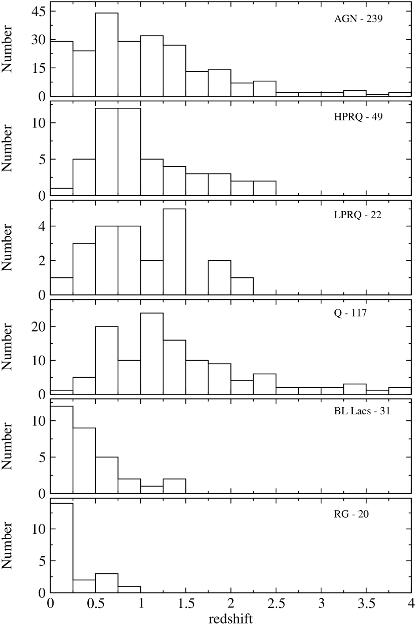
Figure 1: Distribution of redshifts of the MOJAVE/2cm AGN is shown in the top panel. Other panels show the distributions of redshifts for different spectral types of AGN.

The summary of spectroscopic classification from VV03 AGN catalog is presented in Table 1. The full sample consists of 188 quasars, 36 BL Lacs, 20 radio galaxies (RG), and 6 sources with no optical identification (see Table 0.9 Appendix 0.9). Among quasars there are 49 high polarized quasars (optical polarization $P>3$%, HPRQ), 22 low polarized quasars ($P<3$%, LPRQ), and 117 quasars without optical polarimetry information (Q).

The distributions of redshifts of 239 MOJAVE/2cm AGN and individual types of AGN are shown in the different panels of Figure 1. The AGN redshift range is 0.004$\,\leq\,z\,\leq\,$3.8 and the mean redshift is 1.1.

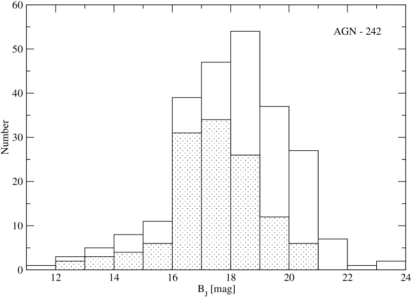
Figure 2: Distribution of apparent B-magnitudes of the MOJAVE/2cm AGN. The dotted histogram represents the $\sim$50% of the sources that have spectrophotometric data.

The apparent B-magnitude in the Johnson’s photometric system, $B_{J}$, for 242 MOJAVE/2 cm sources is shown in Figure 2, where the dotted area shows sources with spectrophotometric data, which represents $\sim$50% of the sample. The remaining sources are too faint for spectroscopy with 2m-class telescopes. The peak of the distribution is at $B_{J}=18.0$ and 11.1$\,\leq B_{J}\leq\,$23.7.

0.3 Optical luminosities

In this work we estimate the optical luminosity at 5100Å ($\lambda\,L_{5100}$) for 233 sources of MOJAVE/2cm compact radio sources drawn for the photometric data available for each AGN. We report as well the spectroscopical parameters of the continuum emission and diverse emission lines, measured directly from the data of 123 AGN of the same sample depending on the redshift of the source. The procedure to obtain $\lambda\,L_{5100}$ is described below, while the treatment of the spectroscopical data is explained in section § 0.6.

The luminosity at 5100Å is estimated using the following expression (e.g., marziani03a):

$$\lambda L_{5100}=3.137\times 10^{35-0.4(M_{\rm{B}}-A_{\rm B})}\,\mathrm{erg\,s^{-1}},$$ (1)

where $A_{\rm B}$ is the galactic extinction in the B-band taken from the NASA Extragalactic Database, and $M_{\rm B}$ is the absolute magnitude given by SG83:

$$M_{\mathrm{B}}={B_{J}}-5\,\mathrm{log\,}d_{L}+2.5\,(1+\alpha_{op})\,\log\,(1+z)+$$

$$5\,\log\,(h)-42.386.$$ (2)

In this equation $h=H_{0}/100$ km s^-1 Mpc^-1 = 0.7; the term $2.5\,(1+\alpha_{op})\,\log\,(1+z)$ reflects the effect of the redshift on measurements through a fixed color band. We adopted an optical spectral index $\alpha_{op}=-0.5$ ($S_{\nu}\propto\nu^{\alpha}$) typical value for radio-loud objects (see Table 2 B01). Finally, $z$ is the redshift, and $d_{L}$ is the luminosity distance for the flat cosmology model given by

$$d_{L}=\frac{c}{H_{0}}(1+z)\left[\eta(1,\Omega_{\rm m})-\eta\left(\frac{1}{1+z},\Omega_{\rm m}\right)\right],$$ (3)

where $\Omega_{\rm m}$=0.3 and $\eta$ is a function of $z$ and $\Omega_{\rm m}$ (see Pen99).

The details on the calculation of ${B_{J}}$ and the procedure to correct by the host galaxy contribution is described in arshakian10.

The distribution of $\lambda\,L_{5100}$ covers 5 orders of magnitude in luminosity with a range between $2\,\times\,10^{42}\,\rm erg\,s^{-1}$ and $1\,\times\,10^{47}\,\rm erg\,s^{-1}$, with an average value of $9\,\times\,10^{45}\,\rm erg\,s^{-1}$; as is shown in Figure 3 for the different AGN types in our sample. The radio galaxies are the sources with weaker luminosities as compared with the quasars and BL Lacs. The distributions of the optical nuclear luminosities for HPRQ and LPRQ show slightly different ranges: $\lambda\,L_{5100,\rm\,HPRQ}$ = $(10^{43}-10^{46})\,\rm erg\,s^{-1}$ and $\lambda\,L_{5100,\rm\,LPRQ}$ = $(10^{44}-10^{46})\,\rm erg\,s^{-1}$. The Kolmogorov-Smirnov test (KS) shows that the null hypothesis that these distributions are drawn for the same parent population cannot be rejected at a confidence level 93% ($P_{KS}=0.072$), for M1 sample the confidence level is 81%, ($P_{KS}=0.189$). It is well known that HPRQ fall within the group of blazars and are known to exhibit a different behavior regarding LPRQ, and their differences cannot be explained with a model based solely on orientation effects. For example, lister00 found that the cores of the LPRQ tend to be less luminous at 15 GHz than the HPRQ. Besides, they reported that the jet components in the LPRQ have magnetic fields parallel to the jet, while those of HPRQ are perpendicular to the flow of the jet. We agree that high– and –low polarized quasars are intrinsically different sources, but more observational data (polarization studies) are needed to understand the physical nature of the differences showed in these two types of quasars.

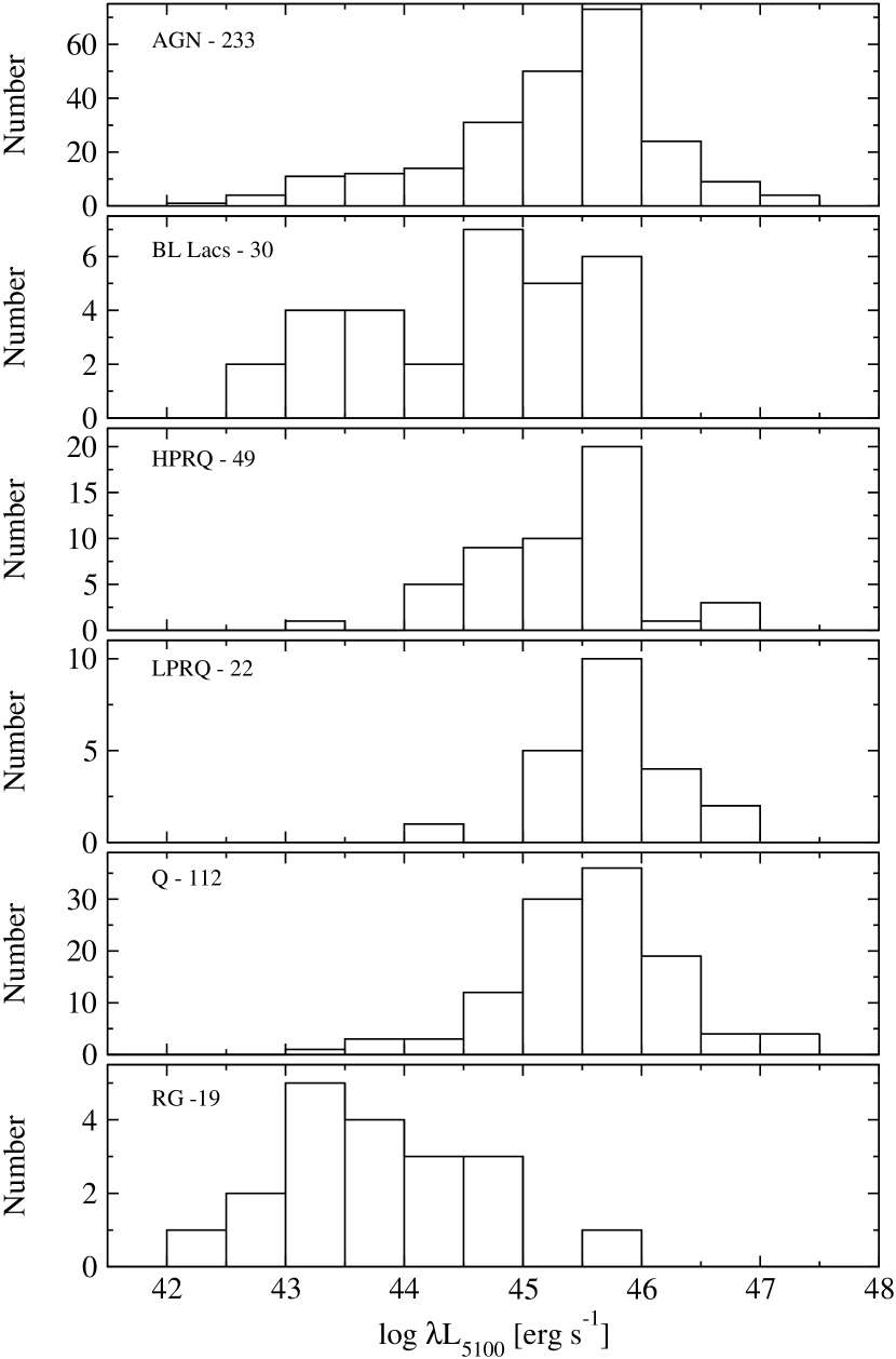
Figure 3: The distribution of corrected photometric optical luminosities at 5100 Å  for the sample of 233 AGN for the MOJAVE/2cm sample (top panel), 30 BL Lacs, 49 HPRQ, 22 LPRQ, 112 quasars, 19 radio galaxies, and 1 unidentified source.

0.4 Spectroscopic Observations and Supplementary Data

Optical spectra of the bright fraction (B $<$ 18) of AGN of the sample were obtained in several observing runs from 2003 to 2006 with two optical telescopes in Mexico: the 2.1m telescope of the Observatorio Astronómico Nacional in San Pedro Mártir, Baja California (OAN–SPM), and the 2.1m telescope of the Observatorio Astronómico Guillermo Haro, in Cananea, Sonora (OAGH). From these telescopes we obtained a total of 146 good quality spectra: 110 from OAN–SPM and 36 from OAGH.

The OAN–SPM spectra were obtained with a Boller & Chivens spectrograph, using a 2.5   slit, a CCD SITe3 (1024 $\times$ 1024 pixels of 24 $\times$ 24 ), a plate scale of 40 /mm), a 300 l/mm grating and blaze angle of $5^{\circ}50^{\prime}$ for the 4000–8000 Å  spectral region, obtaining an effective spectral resolution of $\sim$ 8–10Å.

The OAGH spectra were obtained with a Boller & Chivens spectrograph, using a 2.5   slit, a CCD Tektronix TK1024 (1024 $\times$ 1024 pixels of 24 $\mu$m $\times$ 24 $\mu$m) and a plate scale of 8.18 /mm, a 150 l/mm grating and blaze angle of $3^{\circ}00^{\prime}$ for the 4000–7100 Å  spectral region, obtaining an effective spectral resolution of $\sim 10-15$ Å.

We also searched for spectroscopic data in the archives of the Sloan Digital Sky Survey (SDSS), the Hubble Space Telescope (HST), and in the AGN sample of M03, hereafter M03. The database was also supplemented by spectra kindly provided by C. R. Lawrence (L96, hereafter L96). In total, we found 114 additional spectra: 23 from SDSS, 40 from HST, 36 from L96, and 15 from M03.

Overall, 260 spectra of 123 AGN were analyzed from both our spectroscopic observations and the supplementary data. From these 123 AGN, 73 sources belong to the flux-limited sample MOJAVE-1 (4 BL Lacs, 7 RG, 24 HPRQ, 17 LPRQ, and 21 Q). For this sub-sample we have a total of 104 spectra: 37 from OAN-SPM, 18 from OAGH, 17 from SDSS, 13 from HST, 10 from L96, and 9 from M03.

The typical integration times of our observations were 3600 s splitted in three exposures per source for an object with $B\sim 18$. The spectra for HST, SDSS, L96, and M03 involved typical total integration times of 1000 sec, 3800, 3100, and 10,000 sec, respectively.

Table 2 summarizes the instrumental setup and spectroscopic characteristics of the different sets of optical spectra. Data is organized as follows: Col. (1) is the observing site, Col. (2) is the telescope aperture, Col. (3) is the spectrograph, Col. (4) is the dispersion in Å mm^-1, Col. (5) is the slit width in , Col. (6) is the spectral resolution in Å at FWHM measured on the instrumental profile, and Col. (7) is the number of spectra. Observational details of the spectra obtained from L96 are presented in their Tables 1 and 2, and from M03 is presented in their Table 1. The data of L96 has a spectral resolution in the range between 6–18 Å, and for the data of M03 the spectral resolution is in the range between 3–8 Å.

7

Table 2: Synopsis of optical spectroscopy

				Slit	Spectr.
	Tel.		Grating	Width	Resol.	#
Obs.	Apert.	Spectr.	(l mm-1)	($\arcsec$)	(Å)	spectraa
OAN/SPM	2.1m	B&Ch	300	2.5	8-10	110 (37)
OAGH	2.1m	B&Ch	150	2.5	10-15	36 (18)
SDSS	2.5m	MOSb	420		$\sim 3$	23 (17)
HST	2.4m	FOSc	G270H	2.0	$\sim 2$	40 (13)
aThe numbers in parentheses refer to data acquired from the sample MOJAVE-1. bMOS: multi-object fiber spectrographs with two channels red (420 l mm-1) and blue (640 l mm-1). For specifications see http://www.jhu.edu/~sdss/Spectrographs/OptLayout.html. cSpectral resolution for the HST-FOS data varies depending on the grating and slit width: e.g. G270H– 0.25$\times$2.0$\arcsec$–1.92 Å, G400H –4.3$\arcsec$–2.88Å.

0.5 Data reduction and calibration

The data reduction was performed with the standard procedure using IRAF routines for a long-slit spectroscopy, i.e., bias subtraction, flat-fielding, cosmic-ray removal, and sky subtraction, to produce the final spectra. We also observed standard stars for flux calibration. Wavelength calibration was achieved via observations of HeAr lamp at OAGH and HeAr/CuHeNeAr lamp at OAN–SPM. The arc spectra was obtained after an exposure (if single) or between exposures (if two or more consecutive exposures were taken), with the telescope still pointing towards the target. This calibration was accomplished by fitting a polynomial of suitable order to the pixel wavelength correlation with an uncertainty of $\sim$ 0.5 Å rms for all cases; this was checked using the positions of background night sky lines. Flux calibration was performed using the cataloged spectrophotometric standards stars (massey88; Ok90). Usually, one or two stars at similar airmass of the principal target were observed on the same observing night. Atmospheric extinction correction was applied using the extinction curve for OAN–SPM and OAGH. Objects with more than one observation had their spectra stacked together to increase the signal-to-noise ratio (S/N). The average S/N ratio achieved was approximately 20, 30, and 10 in the continuum near 5100 Å, 3000 Å, and 1350 Å, respectively.

0.6 Analysis of spectra

The general data processing of spectra involved several steps. Once the spectra were flux calibrated, they were shifted to the rest frame of the source with the available redshift data. Then the iron contribution was subtracted and the local continuum emission was fitted with a power law. Finally, the continuum and line parameters were measured. Each of these procedures are described in more detail in the following sections.

0.6.1 Continuum and iron contamination subtraction

Since we are interested in studying the profiles of the emission lines (H$\beta$, Mg 2$\lambda$2798, and C 4$\lambda$1549) it is crucial to subtract the Fe 2 emission in both optical and ultraviolet spectral regions.

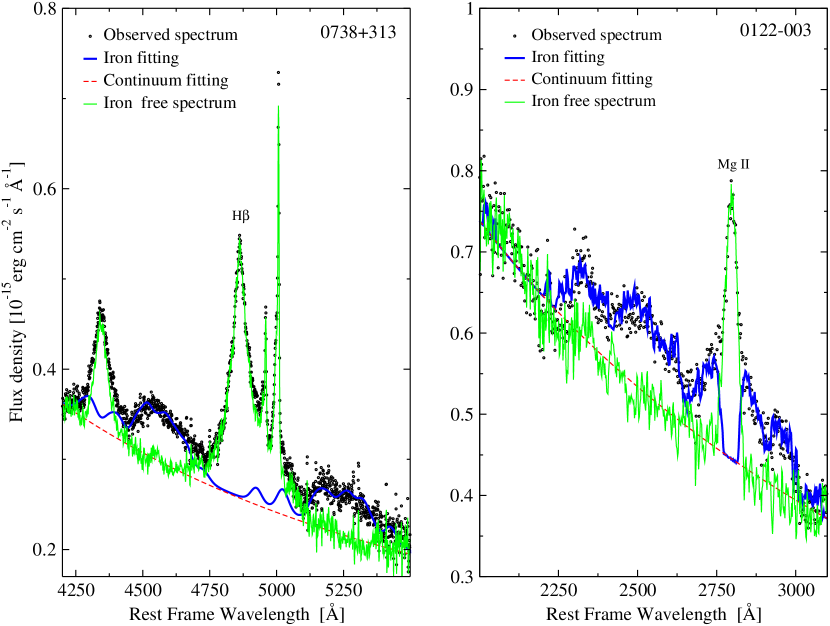
Figure 4: Examples of the subtraction of Fe 2 emission: left panel in the H$\beta$ region for quasar 0738$+$313 and right panel in the Mg ii region for quasar 0122$-$003. It shows the observed spectrum in rest frame (circles); the Fe ii fitting (blue solid line); the power-law continuum fitting (red dashed line); the spectrum after Fe ii subtraction (green solid line). The Mg 2 emission line profile drastically changes after removing the iron contribution.

First, the continuum emission of the rest frame spectra was fitted by a power-law ($a\,\lambda^{b}+c$) in appropriately selected windows and subtracted using the Levenberg-Marquardt least-squares minimal routine. Then, the resulting spectra is compared with the Fe 2 templates in selected spectral regions, which can be modified for the corresponding observed spectral resolution and broadening. The best fit of iron emission is subtracted from the spectra.

The following Fe 2 templates of the NLS1 I Zw 1 galaxy ($z\,=\,$0.0611; FWHM of $\simeq\,$900 km s^-1) were used: (a) the template of VC04 based on spectra from the 4.2 m William Hershel and the 3.9 m Anglo-Australian telescopes for the optical band (from 3575–7530  Å); and (b) the template of VW01, based on spectra from the HST-FOS, for the UV-band (from 1250–3090 Å). These are the more accurate templates available in the literature. The intrinsic narrow lines of this source and its rich iron spectrum make the templates particularly suitable for use with AGN spectra.

Possible continuum windows for each iron region of interest are presented in Table 3. An example of the iron subtraction is illustrated in Figure 4 for two sources in the H$\beta$ and Mg 2 regions.

3 Rest wavelength interval (Å) Emission Line Continuum Fe 2 H$\beta$a 4210–4230 4400–4750 $\lambda$4861 5080–5100 5150–5500 Mg 2a 2220–2230 2300–2650 $\lambda$2798 3010–3040 2900–3090 C 4b 1265–1290 $\lambda$1549 1340–1375 1425–1470 1680–1705 1950–2050 aContinuum windows from K02. bContinuum windows from VP06.

Table 3: Selected continuum and Fe 2 windows

0.6.2 Continuum flux

We obtained the mean value of the continuum emission flux density $f_{\lambda}$ centered at the given wavelength in an interval of $\pm\,50\,$Å  from the iron free spectrum of each AGN. In this manner, we estimated the flux density $f_{5100}$ in the interval 5050 Å$\,<\,\lambda\,<\,$5150 Å, $f_{3000}$ in 2950 Å$<\,\lambda\,<$3050 Å, and $f_{1350}$ in 1300 Å$<\,\lambda\,<$1400 Å. The associated error in the continuum flux density is $\sim$10 % and depends on the S/N ratio of individual spectrum. In few particular cases, where the spectral interval was not enough to get a mean value, we estimated $f_{\lambda}$ by using the power-law $f_{\lambda}$=$a\,\lambda^{b}+c$ that fits the continuum as described in § 0.6.1 above.

0.6.3 Emission-line parameters

The emission lines were fitted with Gaussian profiles (V80), assuming a broad and narrow components, which characterize the kinematics of the broad and narrow line regions (BLR and NLR, respectively). The minimal least-square fitting provides the central position of the Gaussian $\lambda_{c}$, full width at half maximum (FWHM), equivalent width (EW), and line flux.

Four Gaussian components were used for the spectral region of H$\beta$: two for H$\beta$ line (narrow and broad) and two for forbidden lines [O 3] $\lambda\lambda$4959, 5007. The narrow component (NC) of H$\beta$ (H$\beta_{\mathrm{NC}}$) was modelled and subtracted using the Gaussian profile fitted to the [O 3] line, assuming that the [O iii] line ratio [O 3]$\lambda$5007/[O 3]$\lambda$4959 is 2.96 (Os89). In this way, the H$\beta_{\mathrm{NC}}$ FWHM was determined by the [O 3] FWHM. The remaining parameters were set free in the fitting. In particular cases, where the narrow component position was not evident, it was fixed to the central wavelength of the H$\beta$ line. The fitting was done in the spectral interval 4700–5200 Å.

For the Mg 2 and C 4 lines, the restriction used was that the narrow component FWHM$\,\leq\,$2000 km s^-1. This condition was used by MD04, because there is no narrow line in the spectral range that could be modelled to subtract the narrow component from the total line profile. As in H$\beta$, if necessary, the position of the Gaussian NC was fixed in the fitting. Fitting of the Mg 2 and C 4 lines were performed in the spectral ranges 2600–3000 Å  and 1450–1650 Å, respectively. The local continuum in each case was also fitted in the spectral ranges previously mentioned.

The obtained residuals in the fitting compared to the observed spectra were always less than 5 % in the three subsamples. In Figures 5, 6, and 7 an example of the fitting is shown for the lines H$\beta$, Mg 2, and C 4, respectively.

Once the FWHM of the lines was obtained, an instrumental resolution correction was applied by means of the equation:

$$\mathrm{FWHM}_{corrected}=(\mathrm{FWHM}_{observed}^{2}-\mathrm{FWHM}_{instrumental}^{2})^{1/2}$$ (4)

The mean value of the instrumental resolution for the spectra obtained in OAN-SPM and OAGH was $\sim\,$8.5 Å  and $\sim\,$15 Å, respectively. For the SDSS spectra a mean value of $\sim\,$3 Å  was used for the instrumental resolution, and 2 Å  was used for the HST-FOS spectra. The instrumental resolution for the spectra of L96 was obtained from their Table 2, and for M03 spectra it was extracted from their Table 1.

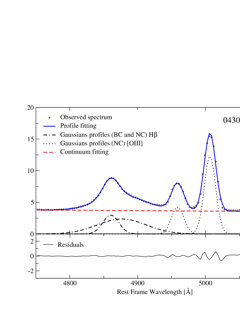
Figure 5: Fitting of the H$\beta$ $\lambda$4861 and [O 3] lines profiles of the AGN 0430$+$052. The abscissa corresponds to the rest wavelength in Å  while the ordinate is the flux density in units of 10^-15 erg s^-1 cm^-2 Å^-1. The upper panel shows the observed spectrum (empty circles), the profile fitting (solid line) comprises by the fitting for 4 Gaussians: 2 for H$\beta$ (dotted lines and points) and 2 for [O 3] $\lambda\lambda$4959,5007 (dotted lines), where the intensity ratio was fixed to 2.96; and the power-law local continuum fitting (dashed line). The width of the narrow component (NC) of H$\beta$ was fixed using the line [O 3] $\lambda$5007. In the lower panel are shown the residuals of the fit, with a mean value of 1.9 % compared to the observed spectra.

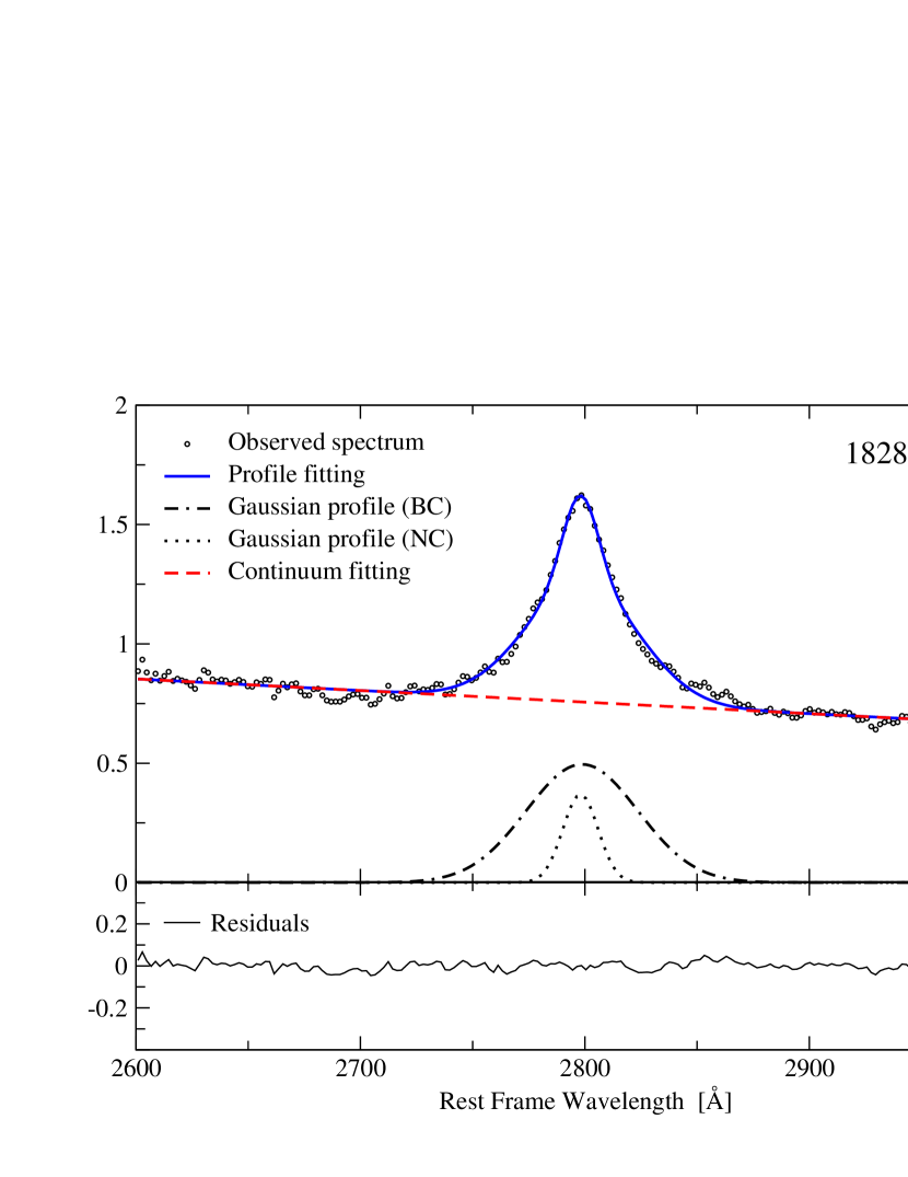
Figure 6: Fitting of the Mg 2$\lambda$2798 line profile for the AGN 1828$+$487. The abscissa corresponds to the rest wavelength in Å  while the ordinate is the flux density in units of 10^-15 erg s^-1 cm^-2 Å^-1. The upper panel shows the profile fitting (solid line) comprises by the fitting with 2 Gaussians curves and the power-law local continuum emission (dashed line). The Gaussian functions represent the broad component (BC, dotted line and points) and the narrow component (NC, dotted line) of the line. The width of the NC was restricted to a FWHM $<$ 2000 km s^-1. In the lower panel are shown the residuals of the fit, with a mean value of 2.4 % compared to the observed spectra.

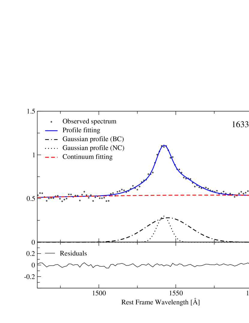
Figure 7: Fitting of the C 4 $\lambda$1549 profile for the AGN 1633$+$382. The symbols are the same as in Figure 5. Also the restriction for the NC was applied to the fit. In the lower panel, the residuals of the fit are shown, with a mean value of 3.4 % compared to the observed spectra.

0.6.4 Continuum and emission line luminosities.

Once we had the continuum and emission line fluxes, the corresponding luminosities were calculated. First, the rest frame flux f_λ was corrected for local reddening, applying the following expression:

$$f_{c}=f_{\lambda}\,10^{({0.4}\,A_{V}\,K_{\lambda})},$$ (5)

where $f_{c}$ is the reddening corrected flux represented by a density flux in the case of continuum emission and integrated flux in the case of line emission. The reddening $A_{V}$ was calculated assuming $A_{V}$=$A_{B}/$1.32, where $A_{B}$ is the $B$-band extinction and $K_{\lambda}$ is estimated from the Galaxy extinction curve of H83. The $A_{B}$ values were obtained from the NED, where dust extinction maps of SFD98 are used, which are based on the infrared difuse emission data from IRAS/DIRBE. The typical extinction for the H$\beta$, Mg 2, and C 4 subsamples is 0.566 mag, 0.342 mag, and 0.547 mag, respectively. The values of $A_{B}$ used are given in Table 0.9 for each AGN.

The luminosity was calculated for the corrected fluxes with the usual relation $L=4\pi\,{d_{L}}^{2}f_{c}$, where $d_{L}$ is the luminosity distance of the object given by equation (3).

0.6.5 Measurement of Fe 2 emission

The identification of iron in the spectra of AGN dates from 40 years ago (e.g., GS64). J87 studied the physical conditions required to explain the observed Fe 2 in AGN spectra. Iron emission measurements in the optical region have shown that this emission (Fe 2_opt) is a distinctive parameter to separate type I from type II AGN (M03). In the ultraviolet W80 showed spectra of intermediate redshift quasars ($z\sim 1$) with prominent Fe 2 emission.

The Fe 2 emission lines can be split into various wavelength bands. In the ultraviolet approximately 2000–3000 Å  and 3000–3400 Å; and in the optical $\sim$4500–4700 Å  and $\sim$5000–5400 Å  (e.g. O77; P78a; J87).

In the optical, the strongest feature, designated as Fe 2 $\lambda 4570$ arises from lines in the range 4470–4670 Å  (see O77; P78a; J87), while other lines contribute to the prominent Fe 2 bands denoted as Fe 2 $\lambda 5190$ and Fe 2 $\lambda 5320$. The AGN redshifts and the instrumental setup used in our sample favours the detection of the Fe 2 $\lambda 4570$ multiplet, which is extensively studied in the literature (e.g. collin00; J87; M03; Z06; zhang07)

The equivalent width of the Fe 2 $\lambda 4570$ emission, denoted as EW(Fe 2 $\lambda 4570$), was calculated via the usual definition EW(Fe 2 $\lambda 4570$)= $f_{FeII}/f_{c}$, where $f_{FeII}$ is the Fe 2 total flux in the spectral range 4450–4600 Å, and $f_{c}$ is the continuum flux intensity measured in the interval 4520–4620 Å. The mean value for the EW(Fe 2 $\lambda 4570$) is 18.2 Å  with a standard deviation of 16.6 Å (c.f. Table LABEL:tab5:average_lines_c).

In the ultraviolet at $\lambda\,<$ 3000 Å, the different regions involve the wings of the Mg 2 $\lambda$2798 emission line. The blue part, in the range 2100–2800 Å, is formed by Fe 2 $\lambda$2100, Fe 2 $\lambda$2500, and Fe 2 $\lambda$2750 (G81) and is denoted as Fe 2 $\lambda 2490$. The first spectral region is also known as Fe 2 $\lambda$2050, the second corresponds to the range 2300–2600 Å, and the third spectral region was named by W80, and partially includes the Mg 2 $\lambda$2798 line. The red part is called Fe 2 $\lambda$2950 and Fe 2 $\lambda$3200. The instrumental setup used and the AGN redshifts limit our study to the blue part of the spectrum. The same procedure used for deriving the Fe 2 $\lambda 4570$ parameters was used to estimated the Fe 2 $\lambda 2490$ parameters. The mean value estimated for EW(Fe 2 $\lambda 2490$) was 54.2 Å  with a standard deviation of 25.8 Å.

0.7 Results

0.7.1 Photometric Data for MOJAVE/2cm AGN Sample

The MOJAVE/2cm sample of 250 AGN is presented in the Appendix 0.9, together with the homogeneous photometric information at the B-band. Table 0.9 is organized as follows: Col. (1) is the source name, Col. (2)–(3) are the J2000.0 coordinates, Col. (4) is the spectroscopic classification from VV03 (B = BL Lac, G = radio galaxy, H = HPRQ, high polarized radio quasar, L = LPRQ, low polarized radio quasars, Q = Quasar with no polarization information), Col. (5) is the redshift, Col. (6) is the B-band extinction taken from NED, Col. (7) is the apparent B magnitude in Johnson’s photometric system, Col. (8) is the absolute B-magnitude, Col. (9) is the MOJAVE monitoring identification (M1, M2 or 2cm; see Table 1), and Col. (10) is the type of the radio spectra between 0.6 GHz and 22 GHz: $\alpha\ga$−0.7 F = flat, $\alpha<$−0.7 S = steep, C = compact steep spectra, G1 = gigahertz-peaked spectrum with one-sided VLBI jets, G2 = gigahertz-peaked spectrum with two-sided VLBI jets.

0.7.2 Spectral Atlas for MOJAVE/2cm AGN Sample

The Spectral Atlas is presented in Appendix LABEL:sec:atlas, it shows 142 spectra corresponding to 123 AGN of the MOJAVE/2cm sample in the observed frame with the redshift information for each source (see Figure LABEL:fig:atlas1). The spectra are ordered by right ascension. If multiple spectra are available for a single source they are presented from blue to red wavelengths.

We present the continuum emission and/or line parameters for 41 sources in the H$\beta$ region, 78 in the Mg 2 region, and 35 in the C 4 region. Also, there are 14 sources with information available for both H$\beta$ and Mg 2 regions, 12 with Mg 2, and C 4, and 5 with H$\beta$, Mg 2 and C 4. The information for the MOJAVE-1 sample that are included in the Atlas are as follows: 28 sources in the H$\beta$ region, 46 in the Mg 2 region, and 23 in the C 4 region. Table 4 summarizes the data presented for each AGN type. Col. (1) is the sample for which we present the spectroscopic data, Col. (2) is the AGN type, Col. (3)–(5) show the different spectral regions of the continuum emission and/or line parameters for which we report data.

6 Spectral Region Sample Spectral Type H$\beta$ Mg 2 C 4 (1) (2) (3) (4) (5) MOJAVE/2cm BL 6 RG 12 2 1 HPRQ 8 19 9 LPRQ 7 18 6 Q 8 39 19 Total 41 78 35 MOJAVE-1 BL 4 RG 7 1 HPRQ 7 16 9 LPRQ 6 14 6 Q 4 15 8 Total 28 46 23

Table 4: Summary of the spectroscopic data

0.7.3 Tabular data

The results of measurements for each parameter of the emission lines and continuum emission for different regions are presented in the Tables LABEL:tabA1:hb1 to LABEL:tabA5:CIV_1 of the Appendix LABEL:secap:parameters. The format of these tables is explained in what follows.

Table LABEL:tabA1:hb1 presents the emission line parameters of the region around H$\beta$ for 41 AGN. Col. (1) is the source name, Col. (2) is the spectrum reference, Col. (3)–(6) are the parameters of the H$\beta$ broad component: FWHM, EW, total flux, and luminosity, respectively, Col. (7)–(10) are the parameters of the [O 3] $\lambda$5007 line: FWHM, EW, flux and luminosity, respectively. Nine of 41 AGN have only narrow emission lines with FWHM H$\beta\lesssim$ 1000 km  s^-1: 0238$-$084, 0316$+$413, 0710$+$439, 0745$+$241, 0831$+$557, 1155$+$251, 1345$+$125, 1642$+$690, and 1957$+$405.

Table LABEL:tabA2:hb2 presents the parameters obtained for the emission continuum 5100 Å  and the Fe 2 $\lambda 4570$: Col. (1) is the source same, Col. (2)–(3) are the flux density and luminosity at 5100 Å, respectively, Col. (4) is the spectral index of the local continuum, Col. (5)–(7) are the total flux, luminosity, and EW of the Fe 2 $\lambda 4570$, respectively.

Table LABEL:tabA3:MgII_1 presents the continuum emission at 3000 Å, and parameters of the Mg 2 $\lambda$2798 emission line for 78 AGN: Col. (1) is the source name, Col. (2) is the spectrum reference, Col. (3)–(6) are the parameters of the Mg 2 broad component: FWHM, EW, total flux, and luminosity, respectively, Col. (7)–(8) are the flux density and luminosity at 3000 Å , respectively, and Col. (9) is the spectral index of the local continuum at 3000 Å.

The emission line parameters of the Fe 2 $\lambda 2490$ are presented in Table LABEL:tabA4:MgII_2: Col. (1) is the source name, Col. (2)–(4) are the total flux, luminosity, and EW, respectively, and Col. (5) is the comment to Fe 2 $\lambda 2490$ measurements.

The continuum emission at 1350 Å  and parameters of the C 4 $\lambda$1549 emission line for 35 AGN are presented in Table LABEL:tabA5:CIV_1: Col. (1) is the source name, Col. (2) is the spectrum reference, Col. (3)–(6) are the parameters of the C 4 broad component: FWHM, EW, total flux, and luminosity, respectively, Col. (7)–(8) are the flux density and luminosity at 1350 Å, and Col. (9) is the spectral index of the local continuum at 1350 Å.

0.7.4 Descriptive statistics for different spectral regions

We have measured the emission line parameters: FWHM, EW, flux, and luminosity, and we obtained the continuum emission flux density and luminosity using our Spectral Atlas of 123 AGN from the MOJAVE/2cm sample. In Table LABEL:tab5:average_lines_c we present the descriptive statistics for each spectral parameter. Columns are as follows: Col. (1) is the parameter, Col. (2) is the spectral type, Col. (3) is the number of sources, Col. (4) is the average value of the parameter, Col.(5) is the standard deviation of the data, and Col. (6) and (7) are the minimum and maximum values of the parameter, respectively. The numbers in parentheses refer to descriptive statistics for the flux-limited sample MOJAVE-1 (M1).

The statistical parameters of the H$\beta$ region are presented for both radio galaxies and quasars because the data for each spectral type are scarce (4 Galaxies, 7 HPRQ, 7 LPRQ, and 6 Q). Note that the radio galaxy 3C 390.3 was excluded from the analysis because of large FWHM H$\beta\,\rm(BC)\sim\,12,000\,km\,s^{-1}$, as well the BL Lacs and the narrow line objects. The C 4 region (9 HPRQ, 6 LPRQ, and 19 Q) was treated similarly. For the Mg 2 region the statistical analysis was performed for different types of quasars (19 HPRQ, 18 LPRQ, and 39 Q). In this case, two radio galaxies were excluded: 0007$+$106 and 3C 390.3.

The broad component of the emission line C 4 has a larger FWHM C 4 (BC) = 6498$\,\pm\,$1515  km s^-1 value, between H$\beta$ and Mg 2. A caveat here is that the data of each emission line corresponds to a different AGN, and only few sources have data for more than one emission line, as was mentioned in § 0.7.2.

The continuum luminosity at $\lambda\,L_{1350}$ is larger by a factor of $\sim 5$ and $\sim 30$ than the continuum luminosities $\lambda\,L_{3000}$ and $\lambda\,L_{5100}$, respectively.

The FWHM of Mg 2 is quite similar for different types of quasars (HPRQ, LPRQ, and Q). This parameter has an average value of FWHM Mg 2$\rm\,(BC)\,=\,$5108$\,\pm\,$946 km s^-1. In contrast, the EW of Mg 2$\rm\,(BC)\,=\,$42$\,\pm\,$29 Å  shows a small difference between types. This parameter for quasars with no polarimetry information (Q) is smaller by 36% and 25% than those for HPRQ and LPRQ. The KS-test shows that the EW of the Mg 2 distributions of the HPRQ and LPRQ are different at a confidence level of 95.1% ($P_{KS}=0.049$), also the distributions of the HPRQ and Q are different at a confidence level of 97.8% ($P_{KS}=0.011$).

Finally, the KS-test between the EW Fe 2 $\lambda$2490 distributions of the HPRQ and LPRQ showed no significant difference ($P_{KS}=0.314$).

Further analysis related to the emission lines parameters and the properties of the pc-scale jets will be presented in a forthcoming paper.

Table 5: Mean values of parameters for continuum and line emission

Parameter	Type	Number	Average	$\sigma$	Min.	Max.
(1)	(2)	(3)	(4)	(5)	(6)	(7)
FWHM H$\beta\rm\,(BC)$ [km s-1]	All	24	4055	1331	1670	8600
		(20)	(3957)	(856)	(2650)	(5750)
EW H$\beta\rm\,(BC)$ [Å]	All	24	56	24	13	125
		(20)	(57)	(26)	(13)	(125)
$L_{\rm H\beta\rm\,(BC)}$ [1042 erg s-1]	All	24	40	50	1	182
		(20)	(37)	(44)	(1)	(182)
EW Fe 2 $\lambda$4570  [Å]	All	22	18	17	2	69
		(17)	(19)	(17)	(2)	(69)
$L_{4570}$ [1041 erg s-1]	All	22	96	96	2	342
		(17)	(98)	(99)	(2)	(342)
FWHM [O 3] $\lambda$5007 [km s-1]	All	35	767	382	360	1716
		(24)	(731)	(328)	(360)	(1394)
EW [O 3] $\lambda$5007 [Å]	All	35	39	62	0.2	380
		(24)	(43)	(75)	(5)	(380)
$L_{[{O\textsc{3}}]}$ [1042 erg s-1]	All	35	14	33	0.004	191
		(24)	(10)	(13)	(0.004)	(50)
$\lambda\,L_{5100}$ [1044 erg s-1]	All	41	31	42	0.01	181
		(28)	(34)	(43)	(0.006)	(181)
FWHM Mg 2$\rm\,(BC)$ [km s-1]	All	76	5108	946	2445	8752
		(45)	(5174)	(663)	(3735)	(7495)
	HPRQ	19	5118	960	2565	7495
		(16)	(5272)	(789)	(4245)	(7495)
	LPRQ	18	5151	1063	3735	8752
		(14)	(4991)	(599)	(3735)	(5583)
	Q	39	5083	908	2445	6849
		(15)	(5239)	(578)	(4287)	(6266)
EW Mg 2$\rm\,(BC)$ [Å]	All	76	36	24	6	177
		(45)	(33)	(27)	(6)	(177)
	HPRQ	19	27	18	6	74
		(16)	(29)	(19)	(6)	(74)
	LPRQ	18	31	12	15	53
		(14)	(30)	(11)	(15)	(53)
	Q	39	42	29	11	177
		(15)	(40)	(41)	(13)	(177)
$L_{{Mg\textsc{2}}\rm(BC)}$ [1042 erg s-1]	All	76	177	695	7	6091
		(45)	(229)	(899)	(11)	(6091)
	HPRQ	19	53	34	7	126
		(16)	(50)	(30)	(11)	(126)
	LPRQ	18	476	1407	35	6091
		(14)	(587)	(1591)	(47)	(6091)
	Q	39	99	97	12	438
		(15)	(85)	(60)	(17)	(196)
EW Fe 2 $\lambda$2490 [Å]	All	67	54	26	6	128
		(40)	(50)	(26)	(6)	(128)
	HPRQ	18	41	21	6	79
		(15)	(39)	(22)	(6)	(79)
	LPRQ	16	47	17	18	74
		(12)	(47)	(17)	(18)	(67)
	Q	33	65	27	21	128
		(13)	(64)	(33)	(22)	(128)
$L_{2490}$ [1042 erg s-1]	All	67	1614	10,772	31	88,402
		(40)	(2456)	(13,941)	(40)	(88,402)
	HPRQ	18	137	101	40	451
		(15)	(118)	(68)	(40)	(275)
	LPRQ	16	5863	22014	36	88402
		(12)	(7760)	(25,400)	(100)	(88,402)
	Q	33	359	535	31	2760
		(13)	(257)	(153)	(46)	(521)
$\lambda\,L_{3000}$ [1044 erg s-1]	All	76	204	936	8	8205
		(45)	(287)	(1212)	(8)	(8205)
	HPRQ	19	88	70	13	237
		(16)	(84)	(70)	(13)	(237)
	LPRQ	18	592	1905	23	8205
		(14)	(735)	(2155)	(33)	(8205)
	Q	39	82	90	8	386
		(15)	(84)	(73)	(8)	(223)
FWHM C 4$\rm\,(BC)$ [km s-1]	All	34	6498	1515	2818	9150
		(23)	(6640)	(1500)	(3445)	(9150)
EW C 4$\rm\,(BC)$ [Å]	All	34	29	17	10	87
		(23)	(29)	(17)	(10)	(87)
$L_{{C\textsc{4}}\rm\,(BC)}$[1042 erg s-1]	All	34	817	2063	20	11,345
		(23)	(857)	(2314)	(27)	(11,345)
$\lambda\,L_{1350}$ [1044 erg s-1]	All	34	983	3363	5	19,566
		(23)	(1199)	(4043)	(24)	(19,566)

0.8 Summary

For the first time an optical spectroscopic atlas with intermediate resolution data of the bright part of the MOJAVE/2cm sample, comprised by core-dominated AGN at 15 GHz, is presented.

The parameters obtained from the spectra of 123 sources, such as FWHM, EW, fluxes, and luminosities of various emission lines (H$\beta$, [O 3] $\lambda$5007, Mg 2 $\lambda$2798, and/or C 4 $\lambda$1549), and their corresponding continuum emission are presented together with the descriptive statistics of these parameters. The luminosities and equivalent widths of the Fe II $\lambda$4570 and Fe 2 $\lambda$2490 are presented for 22 and 67 sources, respectively.

We also carried out a photometric calibration that allowed us to present a homogeneous B–band photometric data for 242 AGN of the MOJAVE/2cm sample. Using these data, arshakian_2_10; arshakian10 have discussed the relations between optical, radio, and $\gamma$-ray emission of 135 AGN from the flux-density-limited MOJAVE-1 sample. torrealba11 used the photometric data of 233 AGN of the MOJAVE/2cm sample to confirm the relations between the optical and 15 GHz emission found for MOJAVE-1. In a forthcoming paper, we will present the results of analysis of the emission line parameters and the properties of the pc-scale jets. Preliminary results about this study have been published in A05, torrealba08, torrealbaphd2010, and hovatta10.

0.9 MOJAVE/2cm AGN sample

10 MOJAVE/2cm AGN SAMPLE