Quantum spin Hall effect in 2D topological insulators

Abstract

The original motivation of great interest to topological insulators was the hope to observe the quantum spin Hall effect. Therefore if a material is in the topological insulator state they frequently call it the quantum spin Hall state. However, despite impressive experimental results confirming the existence of the quantum spin Hall state, the quantum spin Hall effect has not yet been detected. After a short overview of what was originally suggested as the quantum spin Hall effect (quantum spin conductance determined by the topological Chern number) the paper analyzes the crucial role of the boundary condition on the observation of the effect and finally discusses whether and how the quantum spin Hall effect could be observed.

1 Introduction

Topological insulators have recently attracted great attention and their study is developing into a new exciting area of condensed matter physics[1, 2, 3, 4, 5, 6, 7, 8, 9, 10]. The key feature of topological insulators is the presence of helical edge states in 2D systems (or surface states in 3D systems). The edge states cross the whole forbidden gap separating the valence-band and the conduction-band bulk continua. Helicity of edge states means that electrons with the same spin can move only in one direction, which is opposite for two spin directions. As a result, the edge states are robust against elastic backscattering, which conserves spin, and the electron transport along edges becomes ballistic. The edge state of the 2D topological insulator were experimentally detected in the HgTe quantum well [5] by studying charge transport. It was demonstrated that at the quantum well thickness exceeding the critical value 6.3 nm there was an interval of gate voltages where the conductance reaches the quantum conductance value independently of the sample width $W$ (see Fig. 1). This is a clear evidence of the ballistic transport through edge states while the main bulk is not conducting. The topological insulators states were also detected in 3D materials [8, 9, 10]. Though nowadays topological phases are mostly investigated in solids they were already well known in superfluid ³He from 80s [11].

Originally 2D topological insulators were introduced as systems, in which the quantum spin Hall effect (QSH) was expected [1, 3], and the state of the topological insulator is frequently called the QSH state. However, it is necessary to clearly specify the definition of the spin Hall effect in general and the quantum spin Hall effect in particular. Historically the phenomenon, which is called nowadays spin Hall (SH) effect, was defined as an edge spin accumulation resulting from a bulk spin current transverse to an external electric field [12]. At the sample boundary, which fully reflects all electrons, the spin current induced by the electric field must be compensated by a spin diffusion current. Spin diffusion is a dissipative process, which is related with non-equilibrium spin accumulation at the edge (or spin orientation in the terminology of Dyakonov and Perel [12]). Since spin accumulation is more accessible for observation than spin current, usually observation of spin accumulation is considered as an experimental confirmation of the SH effect [13, 14]. But later it was revealed that spin accumulation is not an ideal probe of bulk spin currents since spin accumulation is possible without bulk spin current, and, vice versa, spin current not necessarily results in spin accumulation (see the review [15] and references therein). This is a consequence of non-conserved total spin. In particular, at the equilibrium bulk spin currents cannot lead to spin accumulation, since the latter is accompanied by dissipation. Instead spin is transformed to an orbital moment at the sample edge (edge torque[16]). The same is true for bulk spin currents in insulators: since an external electric field does not pump energy into the sample (no Joule heating) dissipative spin accumulation cannot be supported.

The adjective ”quantum” was added to the SH effect in the topological insulators in order to stress that the spin conductance (ratio of the bulk transverse spin current to the electric field) was universally determined by the topological Chern number for the 2D Brillouin zone [3]. Such a QSH effect has not yet been detected, since the author is not aware of any measurement, which probes anything connected with the bulk spin conductance and no experiment up to now is able to detect the predicted quantum spin conductance in the topological phase. Nevertheless, it is believed that the QSH effect has already been observed [4]. The ingenious experiments of König et al. [5] definitely confirmed existence of ballistic edge states and revealed the quantum charge conductance but there were no direct or indirect evidences of quantum spin conductance simply because nothing dependent on spin was measured. Though both, the ballistic edge states (and the quantum charge conductance as a result of it) and the quantum spin conductance, originated from topology, the common origin does not make two phenomena identical. An essential progress in studying spin-related phenomena in topological insulators was recent detection of spin polarization of the edge states [17] using the inverse SH effect, but this new impressive achievement still does not provide any information on bulk quantum spin conductance, since the latter does not affect any measurement result. So the QSH effect, at least in its original meaning, still waits its experimental confirmation.

The present paper elaborates this point of view. It starts from a short overview of the model by Bernevig, Hughes, and Zhang (BHZ) for the topological insulator (Sec. 2) and the definition of spin and spin current in this model (Sec. 3). In Sec.  4 the quantum spin conductance for the periodic boundary is discussed, which is determined by the topological Chern number and was originally considered as the determining feature of the QSH effect. Section 5 shows that in the strip geometry with fully reflective lateral edges it is impossible to realize the quantum spin conductance. But in this geometry there is non-quantum spin conductance, which is possible both in the topological and conventional-insulator phases of the BHZ model. Section 6 addresses spin accumulation (polarization) at edge states and argues that observation of spin polarization cannot be considered as demonstration of the QSH effect. The concluding Sec. 7 discusses a possibility to detect the genuine QSH effect using the Corbino geometry and summarizes the present analysis: the QSH effect is still waiting its experimental confirmation.

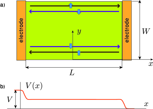
Figure 1: Voltage biased topological insulator. (a)Edge states. Wide arrows show spin direction (spin quantization axis is not in the plane as in the figure). At the upper edge rightmovers have spin s up while leftmovers have spins down. At the lower edge directions of motion are opposite. (b) Voltage variation between electrodes. The voltage varies only near electrodes whereas inside the sample there is no electric field because of ballistic transport along edge channels.

2 The topological-insulator model of Bernevig, Hughes, and Zhang

The simplest and therefore the most transparent model for studying fundamental features of the topological insulator is the model suggested by Bernevig, Hughes, and Zhang (BHZ) for the topological insulator in the HgTe quantum well [3, 4, 18]. The model is a simplified version of the Kane model and its 4$\times$4 Hamiltonian is given by

$${\cal H}=\left(\begin{array}[]{cc}\hat{H}({\bm{k}})&0\\ 0&\hat{H}(-{\bm{k}})^{*}\end{array}\right),$$ (1)

where

$$\hat{H}({\bm{k}})=\varepsilon(k)\hat{I}+d_{i}\hat{\tau}_{i}$$ (2)

is a 2$\times$2 Hamiltonian, $\hat{\tau}_{i}$ are Pauli matrices of the pseudospin, $i=x,y,z$, and $\hat{I}$ is a unit $2\times 2$ matrix. Assuming that all essential processes occur at low $k$ close to the Brillouin zone center, the components $d_{i}$ of the vector $\bm{d}$ are

$$d_{x}=Ak_{x},~{}~{}d_{y}=Ak_{y},~{}~{}d_{z}=\epsilon_{0}(k)=M-Bk^{2}.$$ (3)

Two components of the pseudospin in any $2\times 2$ block of the Hamiltonian (1) correspond to the valence (pseudospin up) and the conduction (pseudospin down) bands, which overlap in the topological insulator phase at $M>0$. The off-diagonal linear in ${\bm{k}}$ terms in any block lead to mixing of two original bands and to forming new bands separated by a forbidden gap. The conventional-insulator phase without edge states corresponds to the condition $M<0$. Further we shall neglect $\varepsilon(k)$ in the Hamiltonian (2) as not important for the outcome of the analysis [4].

The lower block yields the states obtained from those for the upper block by the time-reversal transformation. Because of the absence of off-diagonal blocks in the Hamiltonian (1), one can analyze states for any block separately. We consider the upper block. The eigenstates in the ${\bm{k}}$ space for the Hamiltonian (2) are spinors

$${\bm{\Psi}}_{\pm}(k_{x},k_{y})={1\over\sqrt{2\epsilon}}\left(\begin{array}[]{c}\sqrt{\epsilon\pm\epsilon_{0}}\\ \pm{A(k_{x}+ik_{y})\over\sqrt{\epsilon\pm\epsilon_{0}}}\end{array}\right),$$ (6)

where $\epsilon=|{\bm{d}}|=\sqrt{\epsilon_{0}^{2}+A^{2}k^{2}}$, and the spinors ${\bm{\Psi}}_{+}$ and ${\bm{\Psi}}_{-}$ correspond to the energies $+\epsilon$ and $-\epsilon$ respectively. At $M<A^{2}/2B$ the energy of the upper band has a minimum at $k=0$ (Fig. 2a). At $M>A^{2}/2B$ the energy has a maximum at $k=0$, whereas the minimum band energy $\epsilon_{m}=A\sqrt{M/B-A^{2}/4B^{2}}$ corresponds to $k_{m}=\sqrt{M/B-A^{2}/2B^{2}}$ (Fig. 2b).

An edge state near the edge $y=0$ should be a a superposition of two states of the same energy and $k_{x}$:

$${\bm{\Psi}}=\left[a_{1}{\bm{\Psi}}_{+}(k_{x},k_{y1})e^{ik_{y1}y}+a_{2}{\bm{\Psi}}_{+}(k_{x},k_{y2})e^{ik_{y2}y}\right]e^{ik_{x}x},$$

where $k_{y1}$ and $k_{y2}$ are two complex solutions with positive imaginary parts of the bi-quadratic equation for $k_{y}$ following from the energy spectrum at fixed $\epsilon$ and $k_{x}$.

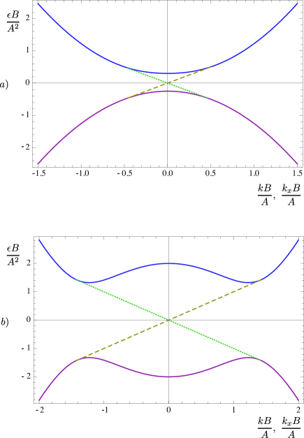
Figure 2: Band energy as a function of $k$ (solid lines) and edge state energy as a function of $k_{x}$ (dotted and dashed lines) in a topological insulator ($M>0$). Dashed and dotted lines correspond to opposite spin directions [upper and and lower block of the Hamiltonian (1)]. a) $M=0.3A^{2}/B<A^{2}/2B$; b) $M=2A^{2}/B>A^{2}/2B$.

The condition ${\bm{\Psi}}=0$ at the edge $y=0$ yields two equations for $a_{1}$ and $a_{2}$, which have a solution if

$$\frac{A(k_{x}+ik_{y1})}{\epsilon_{e}+\epsilon_{0}(k_{1})}=\frac{A(k_{x}+ik_{y2})}{\epsilon_{e}+\epsilon_{0}(k_{2})}.$$ (8)

For $M>0$ this equation is exactly satisfied if $\epsilon_{e}=-Ak_{x}$, which corresponds to the edge state

$${\bm{\Psi}}\propto\left(\begin{array}[]{c}1\\ 1\end{array}\right)e^{ik_{x}x}\left(e^{-p_{+}y}-e^{-p_{-}y}\right),$$ (11)

where $p_{\pm}=A/2B\pm\sqrt{k_{x}^{2}-M/B+A^{2}/4B^{2}}$. Considering the lower block of the Hamiltonian (1) one receives the spectrum $\epsilon_{e}=Ak_{x}$.

3 Spin and spin current in the BHZ model

Starting the analysis of spin currents and accumulation, it is necessary to understand what “spin” we would like to focus on. In HgTe the conduction band originates [3, 4] from a $s$-type ($l=0$) atomic orbital, and its total moment coincides with spin, whereas the valence band is related to a $p$-type ($l=1$) atomic orbital and has the total moment $j=3/2$ with its projection on the quantization axis (the axis $z$ normal to the insulator plane) $m_{j}=1/2$. This projection of the mechanical total angular momentum was also called spin in the previous works [3, 4]. We shall adopt this extension of the term “spin” remembering that in general this is an effective spin but not genuine one. According to this definition the spins in the valence and the conduction bands in HgTe are equal to the electron spin $\hbar/2$. However, the mechanical moment would be relevant only if the theory addressed a mechanic effect, like that considered in Ref. [16]. If the goal is to describe electromagnetic phenomena like the Kerr effect or any other electrodynamic effect, one should use the magnetic moment, which depends on the Lande factor of the atomic orbital. The magnetic moments in the the conduction and valence bands of HgTe are $\mu_{B}$ and $2\mu_{B}/3$, where $\mu_{B}=e\hbar/2mc$ is the Bohr magneton. In order to take it into account we further generalize the definition of effective spin, introducing “spins” $s_{c}$ and $s_{v}$ for the conduction and the valence bands. If the analysis addresses a mechanical effect then $s_{c}=s_{v}=\hbar/2$ in HgTe quantum wells as was supposed earlier [3, 4]. But if the magnetic moment is relevant for the theory, we define effective spins of the conduction and the valence bands as $s_{c}=\hbar/2$ and $s_{v}=\hbar/3$, i.e., as magnetic moments of the bands divided by the electron gyromagnetic ratio. So in general the band effective spins $s_{c}$ and $s_{v}$ differ and the operator of the effective spin in the BHS model is given by [19]

$$\hat{s}^{z}=\bar{s}^{z}\hat{I}+\Delta s^{z}\hat{\tau}_{z},$$ (12)

where $\bar{s}^{z}=(s_{c}+s_{v})/2$, and $\Delta s^{z}=(s_{v}-s_{c})/2$.

Let us consider now the balance equation for spin (the continuity equation with the torque term) for an arbitrary quantum state in the BHS model. The balance equation can be derived from the Schrödinger equation as was explained in details for the Rashba Hamiltonian [15]. Restricting ourselves with the $z$ component of the spin density $S_{z}={\bm{\Psi}}^{\dagger}\hat{s}^{z}{\bm{\Psi}}$, the balance equation is

$${\partial S_{z}\over\partial t}+\nabla_{\alpha}J^{z}_{\alpha}=G^{z},$$ (13)

where the torque is

$$G^{z}=i\Delta s^{z}A\left\{{\bm{\Psi}}^{\dagger}\cdot[\vec{\nabla}\times{\bm{\tau}}]_{z}{\bm{\Psi}}+[\vec{\nabla}\times{\bm{\tau}}]_{z}{\bm{\Psi}}^{\dagger}\cdot{\bm{\Psi}}\right\},$$ (14)

and the spin current is given by

$$J_{i}^{z}={1\over 2}{\bm{\Psi}}^{\dagger}\left\{\hat{s}^{z}\hat{v}_{i}+\hat{v}_{i}\hat{s}^{z}\right\}{\bm{\Psi}}=\bar{s}^{z}{\bm{\Psi}}^{\dagger}\hat{v}_{i}{\bm{\Psi}}+\Delta s^{z}v_{0i}{\bm{\Psi}}^{\dagger}{\bm{\Psi}}.$$

(15)

Here

$$\hat{v}_{i}={\partial\hat{H}({\bm{k}})\over\hbar\partial k_{i}}=v_{0i}(k)\hat{\tau}_{z}+A\hat{\tau}_{i}$$ (16)

is the group velocity operator and $v_{0i}(k)=\partial\epsilon_{0}/\hbar\partial k_{i}$.

The first term in the spin current Eq. (15) differs from the charge current

$$J_{i}=e{\bm{\Psi}}^{\dagger}\hat{v}_{i}{\bm{\Psi}}$$

(17)

by the constant factor $\bar{s}^{z}/e$. Only this term was taken into account in previous publications assuming $\Delta s^{z}=0$. In this approximation our effective spin is a conserved quantity and the torque $G^{z}$ vanishes. But in general the second term proportional to the difference of spins in two bands should not be ignored and leads to important effects as shown below.

An interesting consequence of helical edges in the topological phase $M>0$ is a persistent spin current flowing around the sample. According to Eq. (11), two edge states transport the average spin $\pm\bar{s}^{z}$, and the spin current along the edge is:

$$j^{z}=\bar{s}^{z}(n_{\rightarrow}+n_{\leftarrow})v_{e}.$$ (18)

where $v_{e}=d\epsilon_{e}/\hbar dk_{x}=A/\hbar$ is the group velocity at edge states. This current exists even in the equilibrium [20], when there is no external electric field and the 1D densities $n_{\rightarrow}$ and $n_{\leftarrow}$ of right-moving and left-moving charge carriers are equal. So this is another example of an equilibrium spin current [15].

4 The effect of an electric field: quantum spin conductivity

The QSH effect follows from the calculation of the spin current induced by an electric field using the Kubo approach [3]. The approach is based on the perturbation theory. In the presence of the electric field the perturbation-theory expression for the quantum-state spinors are

$$\tilde{\bm{\Psi}}_{\pm}(k_{x},k_{y})=e^{ik_{x}x+ik_{y}y}\left\{{\bm{\Psi}}_{\pm}+{i\hbar eE\over 4\epsilon^{2}}\hat{v}_{x}{\bm{\Psi}}_{\pm}\right\}.$$ (19)

The transverse spin current in this state follows from its definition by Eq. (15) and is equal to

$$J_{y}^{z}(k_{x},k_{y})=\bar{s}^{z}\left(v_{y}+{i\hbar eE\over 4\epsilon^{2}}{\bm{\Psi}}_{\pm}^{\dagger}[\hat{v}_{y},\hat{v}_{x}]{\bm{\Psi}}_{\pm}\right)+\Delta s^{z}v_{0y}=\bar{s}^{z}\left(v_{y}+{eE\over 2\hbar}{\cal G}\right)+\Delta s^{z}v_{0y},$$ (20)

where the term

$${\cal G}={A^{2}\over\epsilon^{3}}(\epsilon_{0}-\hbar kv_{0})=\hat{\bm{d}}\cdot\left[{\partial\hat{\bm{d}}\over\partial k_{x}}\times{\partial\hat{\bm{d}}\over\partial k_{y}}\right]$$ (21)

is responsible for the topological contribution to the current. Its integral

$$\int{\cal G}d{\bm{k}}=2\pi\left(1+{M\over|M|}\right)=4\pi C$$ (22)

is equal to the area of the spherical surface subtended by the unit vector $\hat{\bm{d}}={\bm{d}}/|{\bm{d}}|$ when integrating over the whole 2D Brillouin zone. Here $C$ is the Chern number, which is equal to 1 in the topological-insulator phase $M>0$, but vanishes in the conventional-insulator phase $M<0$, in full agreement with topological theorems. This is illustrated in Fig. 3.

After integration the single state current (20) over the $\bm{k}$ space and summation of the contributions of the two blocks in the Hamiltonian (1) with opposite directions of spin, only the topological term contributes to the total spin current $J^{z}_{y}=\sigma_{s}E$. Eventually the spin conductance is

$$\sigma_{s}={2e\bar{s}^{z}\over h}C.$$ (23)

This derivation of the quantum spin conductance is well known [3], but it is valid only for periodical boundary conditions.

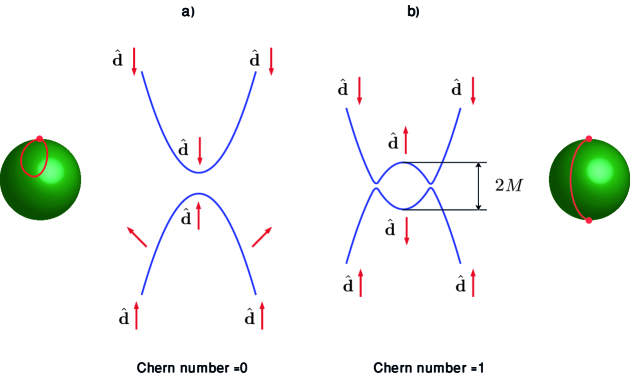
Figure 3: Mapping of the Brillouin zone on the spherical surface of the unit vector $\hat{\bm{d}}=\bm{d}/d$. (a) The conventional insulator, $M<0$. Any path in the Brillouin zone starting in its center and ending at its border maps on the path in the $\hat{\bm{d}}$ space starting and ending at the same pole of the sphere. The total area subtended by the vector $\hat{\bm{d}}$ vanishes. (b) The topological insulator, $M>0$. Any path in the Brillouin zone starting in its center and ending at its border maps on the path in the $\hat{\bm{d}}$ space starting at one pole and ending at the other. The vector $\hat{\bm{d}}$ subtends the whole spherical surface with area $4\pi$.

5 Effect of reflective borders on the bulk spin current

Let us consider now fully reflective edges of the 2D topological insulator. If the spins of two bands are equal, i.e., $\Delta s^{z}=0$ in the expression Eq. (20) for the spin current, the spin current is proportional to the charge current. In the BHZ model spin-flips processes are absent [no off-diagonal blocks in the Hamiltonian Eq. (1)], the total number of electrons with given spin is conserved, and their current normal to the reflective border should vanish. Correspondingly the spin current, which is a counterflow of electrons with opposite spins must also vanish. So the bulk spin current is possible only due to the second term $\propto\Delta s^{z}$ in Eq. (20). A proper eigenfunction near the reflective border is a superposition of an incident and a reflected wave $a_{1}\tilde{\bm{\Psi}}_{\pm}(k_{x},k_{y})+a_{2}\tilde{\bm{\Psi}}_{\pm}(k_{x},-k_{y})$. The superposition must satisfy the condition $|a_{1}|^{2}J_{y}(k_{x},k_{y})+|a_{2}|^{2}J_{y}(k_{x},-k_{y})=0$ imposed by the charge conservation law. Here $J_{y}(k_{x},k_{y})$ is the charge current component normal to the border, which is determined by Eq. (17) for the wave function Eq. (19) taking into account the electric field. In the presence of the electric field $|a_{1}|^{2}$ and $|a_{2}|^{2}$ are not equal. According to Eq. (20) and assuming that the electric field does not change the average density ($|a_{1}|^{2}+|a_{2}|^{2}=2$), the intensities are

$$|a_{1}|^{2}=\left(1-{eE\over 2\hbar}{{\cal G}\over v_{y}}\right),~{}~{}|a_{2}|^{2}=\left(1+{eE\over 2\hbar}{{\cal G}\over v_{y}}\right).$$ (24)

As a result, the term in the spin current proportional to the average spin $\bar{s}^{z}$ vanishes but the term proportional to the spin difference $\Delta s^{z}$ still remains:

$$J_{y}^{z}(k_{x},k_{y})=\Delta s^{z}v_{0y}(|a_{1}|^{2}-|a_{2}|^{2})=\Delta s^{z}{eE\over 2\hbar}{\cal G}{v_{0y}\over v_{y}}.$$ (25)

The total spin current in the whole band does not reduces to the Chern term and is determined by the integral, which does not vanish in a conventional insulator ($M<0$):

$$\int{\cal G}{v_{0y}\over v_{y}}d{\bm{k}}=2\pi\left\{\begin{array}[]{cc}\left(-{A\over 2\sqrt{A^{2}-4MB}}\ln\frac{A^{2}-2MB+A\sqrt{A^{2}-4MB}}{A^{2}-2MB-A\sqrt{A^{2}-4MB}}+\ln{A^{2}-2MB\over 2|M|B}\right)&\mbox{at}~{}M<{A^{2}\over 4B}\\ \left(-{A\over\sqrt{4MB-A^{2}}}\arctan\frac{A\sqrt{4MB-A^{2}}}{A^{2}-2MB}+\ln{A^{2}-2MB\over 2|M|B}\right)&\mbox{at}~{}{A^{2}\over 4B}<M<{A^{2}\over 2B}\end{array}\right..$$ (28)

The parameter $C$ for the periodic and reflective boundary conditions is shown in Fig. 4. Thus, in contrast to the analysis based on plane-wave eigenstates satisfying the periodic boundary condition, the bulk spin current may appear both in the conventional and the topological insulator, and is not governed by the Chern number if the edge of the sample is fully reflective.

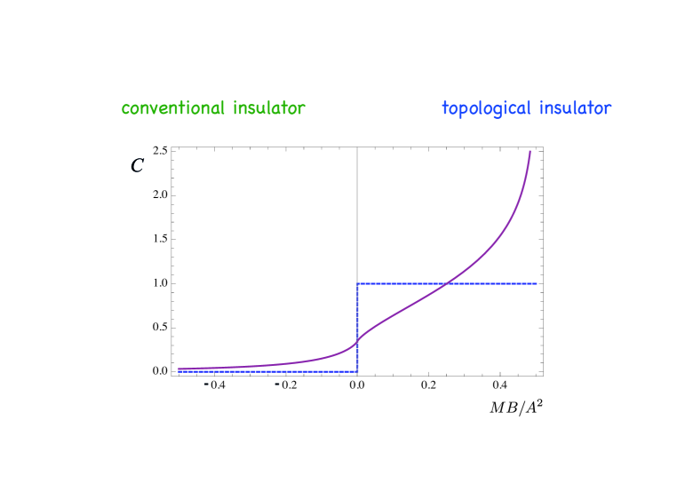
Figure 4: The parameter $C$ determining the spin conductance. For the periodic boundary condition $C$ reduces to the Chern numbers $C=1$ and $C=0$ in the topological and the conventional phases respectively (dotted line). For the reflective boundary condition $C$ is continuous and does not vanish in the both phases (solid line).

6 Bulk spin current and spin accumulation

Observation of the calculated bulk spin conductance in the experiment encounters the problem that in an ideal topological insulator there is no electric field in the bulk since ballistic edge channels, which are robust against elastic scattering, shortcircuit the bulk transforming a topological insulator into a ballistic metal. According to the Landauer–Büttiker theory of ballistic conductors the whole voltage bias between electrodes drops only in the contacts but not in the bulk (see Fig. 1(b)). Correspondingly the bulk spin current linear in the electric field cannot appear and it is impossible to measure quantum spin conductance (i.e., to demonstrate the QSH effect in its original definition) in the strip geometry shown in Fig. 1.

The electric field parallel to the axis $x$ may appear only if there are magnetic impurities at the sample edge, which make carrier backscattering possible and lead to finite conductance of edge channels. However in the absence of the spin conservation law the bulk current not necessarily leads to accumulation. It may result in an edge torque without accumulation, as in the case of equilibrium spin currents in the Rashba medium [15]. As already mentioned in Introduction non-equilibrium spin accumulation is impossible also in insulators since the electric field does not pump energy into the material without longitudinal charge current. The BHZ model is a model of non-interacting electrons, and the band electrons in the bulk and the electrons in the edge states constitute two independent non-interacting ensembles. The bulk band electrons are in the insulating phase and cannot produce any accumulation of spin. Thus independently from whether the electric field and the related bulk spin current do appear inside the sample or do not, it cannot lead to spin accumulation at the edges. Nevertheless, it does not rule out spin accumulation in the edge states, which is inevitably appears due to a rather trivial reason: the voltage drop between electrodes generates a ballistic electric current $J=ev_{e}(n_{\rightarrow}-n_{\leftarrow})$ in edge channels, which leads to inequality of the rightmover and leftmover densities $n_{\rightarrow}$ and $n_{\leftarrow}$. Since rightmovers and leftmovers have opposite spins this leads to spin accumulation (or polarization),

$$S_{z}={\bar{s}^{z}\over ev_{e}}J,$$ (29)

totally independent from what is going on with bulk spin currents. Only the average spin appears in this expression since according to Eq. (11) the edge state is a superposition of two bands with equal amplitudes.

One can rewrite Eq. (29) for the edge spin polarization using the relation connecting the edge channel current $J=(e^{2}/h)V$ with the voltage between electrodes via the charge quantum conductance $e^{2}/h$:

$$S_{z}={\bar{s}^{z}e\over h}{V\over v_{e}}.$$ (30)

where the half of the quantum spin conductance appears as a factor. One may argue that since spin polarization contains the quantum of spin conductance its measurement would be a demonstration of the QSH effect. Such conclusion is at least debatable. The conductance quantum appears in this expression because of charge conductance of the ballistic transport without any connection with the actual bulk spin current, which is proportional to $\Delta s_{z}$ whereas the spin polarization is proportional to the average spin $\bar{s}^{z}$. The choice of the nomenclature is always a matter of taste and convention and one may redefine the QSH effect as the effect of spin polarization. But such a definition would be very far from the original concept of the SH effect [12], which considered accumulation of spin brought to the edge by the bulk spin current linear in the bulk electric field. For comparison, let us mention that the quantum charge conductance appears not only in the quantum Hall (now we mean not spin Hall!) effect, but also in other phenomena, e.g. in the ballistic transport in 1D channels (the edge state is an example of such a channel). But this does not make these phenomena identical to the quantum Hall effect.

7 Conclusion: observation of the genuine QSH effect

The analysis presented above leads to the conclusion that the genuine QSH effect (bulk quantum spin conductance transverse to an external electric field) cannot be detected not only from transport measurements of charge conductance but even from observation of spin polarization at sample edges reported recently [17]. Indeed, the quantum spin conductance determined by the Chern number is not relevant for this observation and was not used for its interpretation. The detection of the QSH effect is possible only if experimentalists are able to probe the bulk spin current in the geometry with the periodic boundary conditions when there are no edges parallel to the electric field and correspondingly no edge spin polarization . There is no doubt that it is a serious challenge for experimentalists. Nevertheless such a geometry can be considered, at least in the theory. Figure 5 shows the Corbino geometry for a HgTe quantum well, where the transition to the topological phase is possible. Applying a radial electric field one creates an azimuthal spin current. The Corbino geometry provides the periodic boundary condition, which allows to observe the quantum spin conductance determined by the Chern number. With help of a local gate (see the figure) one can create a potential barrier, which leads to reflection of electrons propagating azimuthally and therefore can transform the boundary condition from periodic to purely reflective. This would make possible to experimentally check two predictions: quantum spin conductance for periodic boundary conditions, i.e., the genuine QSH effect, and non-quantum spin conductance for reflective boundary condition, which may exist both in a conventional and a topological insulator. An important feature of the Corbino geometry with the periodic boundary condition is that there are no ballistic helical edge channels, which are parallel to the electric field and shortcircuit the electrodes. So the electric field is present in the sample.

The most difficult part is detection of a bulk spin current in the absence of any spin polarization. A possible method of bulk moment current detection is observation of an electric field generated by any moving magnetic moment [15, 21, 22]. This is the “inverse spin Hall effect”, which has already been observed in a number of experiments [23, 24, 25, 26]. But in the geometry of the QSH effect the electric field generated by the spin current is exactly parallel to the external electric field. So measurement of the spin current requires detection of a small correction to the dielectric permeability. The local gate can help to this detection, since it works as a valve, which regulates the spin current and therefore tunes the small correction to the dielectric permeability.

One may also hope to find suitable optical methods of spin-current detection. Recently a second-order nonlinear optical effect of spin currents was revealed theoretically [27] and experimentally [28]. It was demonstrated that a pure spin current, even without spin polarization, is able to induce a second-harmonic generation. Concluding, the experimental detection of the Chern number, which determines the quantum spin conductance, seems elusive at the present moment, and some new ingenious set-ups should be looked for this goal.

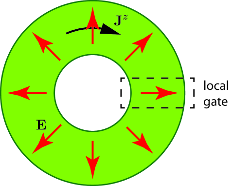
Figure 5: Tentative set up for observation of the QSH effect in the Corbino geometry. The radial electric field $\bm{E}$ induces the azimuthal spin current $\bm{J}^{z}$. Applying the voltage to the local gate (dash-line rectangle) one can create a potential barrier transforming the periodic boundary condition into the reflective one.

- [1] Kane, C. L. and Mele, E. J., “ topological order and the quantum spin Hall effect,” Phys. Rev. Lett. 95, 146802 (2005).
- [2] Kane, C. L. and Mele, E. J., “Quantum spin Hall effect in graphene,” Phys. Rev. Lett. 95, 226801 (2005).
- [3] Bernevig, B. A., Hughes, T. L., and Zhang, S.-C., “Quantum spin Hall effect and topological phase transition in HgTe quantum wells,” Science 314, 1757–1761 (2006).
- [4] König, M., Buhmann, H., Molenkamp, L. W., Hughes, T., C.-X. Liu, X.-L. Q., and Zhang, S.-C., “The quantum spin Hall effect: Theory and experiment,” J. Phys. Soc. Jpn. 77, 031077 (2008).
- [5] König, M., Wiedmann, S., Brúne, C., Roth, A., Buhmann, H., Molenkamp, L. W., Qi, X.-L., and Zhang, S.-C., “Quantum spin Hall insulator state in HgTe quantum wells,” Science 318, 766–770 (2007).
- [6] Moore, J. E., “The birth of topological insulators,” Nature (London) 464, 194–198 (2010).
- [7] Hasan, M. Z. and Kane, C. L., “Colloquium: Topological insulators,” Rev. Mod. Phys. 82(4), 3045–3067 (2010).
- [8] Hsieh, D. et al., “Observation of unconventional quantum spin textures in topological insulators,” Science 323, 919–922 (2009).
- [9] Xia, Y. et al., “Observation of a large-gap topological-insulator class with a single dirac cone on the surface,” Nat. Phys. 5, 398–402 (2009).
- [10] Chen, Y. L. et al., “Experimental realization of a three-dimensional topological insulator, Bi2Te3,” Science 325, 178–181 (2009).
- [11] Volovik, G. E., [The universe in a helium droplet ], Clarendon Press, Oxford (2003).
- [12] Dyakonov, M. I. and Perel, V. I., “Possibility of orienting electron spin with current,” Pis’ma Zh. Eksp. Teor. Fiz. 13(11), 657–660 (1971). [JETP Lett. 13, 467–469 (1971)].
- [13] Kato, Y. K., Myers, R. C., Gossard, A. C., and Awschalom, D. D., “Observation of the spin Hall effect in semiconductors,” Science 306, 1910–1913 (2004).
- [14] Wunderlich, J., Kaestner, B., Sinova, J., and Jungwirth, T., “Experimental observation of the spin-Hall effect in a two-dimensional spin-orbit coupled semiconductor system,” Phys. Rev. Lett. 94, 047204 (2005).
- [15] Sonin, E. B., “Spin currents and spin superfluidity,” Adv. Phys. 59, 181–255 (2010).
- [16] Sonin, E. B., “Proposal for measuring mechanically equilibrium spin currents in the Rashba medium,” Phys. Rev. Lett. 99, 266602 (2007). Erratum: ibid. 105, 149902 (2010).
- [17] Brüne, C., Roth, A., Buhmann, H., Hankiewicz, E. M., Molenkamp, L. W., Maciejko, J., Qi, X.-L., and Zhang, S.-C., “Spin polarization of the quantum spin Hall edge states,” arXiv:1107.0585.
- [18] Zhou, B., Lu, H.-Z., Chu, R.-L., Shen, S.-Q., and Niu, Q., “Finite size effects on helical edge states in a quantum spin-Hall system,” Phys. Rev. Lett. 101, 246807 (2008).
- [19] Sonin, E. B., “Edge accumulation and currents of moment in two-dimensional topological insulators,” Phys. Rev. B 82, 113307 (2010).
- [20] Büttiker, M., “Edge-state physics without magnetic fields,” Science 325, 278–279 (2009).
- [21] Zhang, S., “Probing spin currents in semiconductors,” J. Appl. Phys. 89, 7564–7566 (2001).
- [22] Nagaosa, N., “Spin currents in semiconductors, metals, and insulators,” J. Phys. Soc. Jpn. 77, 031010 (2008).
- [23] Valenzuela, S. O. and Tinkham, M., “Direct electronic measurement of the spin Hall effect,” Nature (London) 442, 176–179 (2006).
- [24] Brüne, C., Roth, A., Novik, E. G., König, M., H. Buhmann, E. M. H., Hanke, W., Sinova, J., and Molenkamp, L. W., “Evidence for the ballistic intrinsic spin Hall effect in HgTe nanostructures,” Nature Phys. 6, 448–454 (2010).
- [25] Ando, K. and Saitoh, E., “Observation of inverse spin–Hall effect in silicon,” arXiv:1107.2585.
- [26] Saitoh, E., Ueda, M., Miyajima, H., and Tatara, G., “Conversion of spin current into charge current at room temperature: Inverse spin–Hall effect,” Appl. Phys. Lett. 88, 182509 (2006).
- [27] Wang, J., Zhu, B.-F., and Liu, R.-B., “Second-order nonlinear optical effects of spin currents,” Phys. Rev. Lett. 104, 256601 (2010).
- [28] Werake, L. K. and Zhao, H., “Observation of second-harmonic generation induced by pure spin currents,” Nat. Phys. 6, 875–878 (2010).