Spatial Pauli-blocking of spontaneous emission in optical lattices

Abstract

Spontaneous emission by an excited fermionic atom can be suppressed due to the Pauli exclusion principle if the relevant final states after the decay are already occupied by identical atoms in the ground state. Here we discuss a setup where a single atom is prepared in the first excited state on a single site of an optical lattice under conditions of very tight trapping. We investigate these phenomena in the context of two experimental realizations: (1) with alkali atoms, where the decay rate of the excited state is large and (2) with alkaline earth-like atoms, where the decay rate from metastable states can be tuned in experiments. This phenomenon has potential applications towards reservoir engineering and dissipative many-body state preparation in an optical lattice.

I Introduction

An atom in free space prepared in an excited electronic state will decay by spontaneous emission to lower lying electronic states. Spontaneous emission is a basic ingredient in light scattering from atoms, and processes involving spontaneous emission constitute fundamental decay, and thus decoherence mechanisms, when manipulating atoms with laser light. There is an extensive literature on suppression of the (free space) spontaneous emission rate. This can be achieved first of all by engineering the density of states of the radiation modes of the emitted photons, e.g. by placing emitters in a cavity Kleppner (1981), in a photonic bandgap material Noda et al. (2007), or close to a surface Jhe et al. (1987). On the other hand, recent experimental advances with quantum degenerate Fermi gases have motivated theoretical studies of “Pauli-blocking” spontaneous emission, where the spontaneous emission of an atom from the first excited electronic state to the ground state is blocked by other fermionic atoms occupying possible final states into which the atom can decay. This scenario and prospects for experimental observation have so far been discussed for a single excited atom above a Fermi sea of many trapped ground state atoms Busch et al. (1998); Shuve and Thywissen (2010), where the condition for Pauli-blocking spontaneous emission is $E_{F}>E_{R}$ with $E_{F}$ the Fermi energy of ground state atoms, and $E_{R}=\hbar^{2}k^{2}/2M$ the recoil energy, where $k$ denotes the wavenumber of the emitted photons and $M$ the atomic mass.

Here we will instead discuss a complementary and conceptually simpler setup, in which a single atom is prepared in the first excited state on a single site of an optical lattice under conditions of very tight trapping realizing the Lamb Dicke limit, i.e. $\eta=2\pi x_{0}/\lambda_{L}\ll 1$ with $x_{0}$ the size of the atomic wavepacket and $\lambda_{L}$ the wavelength of the trapping laser. In this case under suitable conditions, which we discuss below, even a single fermionic atom prepared on the same lattice site in the electronic ground state and motional ground state matching the atom in the excited state can block the dominant decay channel for the excited state to the ground state. Below we will analyze this suppression of decay, in particular in light of the new opportunities opened by recent experiments and theoretical proposals involving fermionic alkaline earth atoms Ye et al. (2008); Derevianko and Katori (2011); Daley et al. (2008); Fukuhara et al. (2009); Cazalilla et al. (2009); Gorshkov et al. (2010); Swallows et al. (2011); Daley (2011), but also with alkali atoms in optical lattices Bloch et al. (2008); Lewenstein et al. (2007); Jaksch and Zoller (2005).

The paper is organized as follows. In Sec. II we give a brief qualitative overview of the atomic decay dynamics and introduce two experimental schemes to observe Pauli-blocked spontaneous emission. Details of these scenarios are discussed in Sec. III. In Sec. IV we study the properties of the emitted photon wavepacket and the possibility to shape its form by preparing the blocking atom in appropriate initial states. We conclude with a summary in Sec. V and also give an outlook towards possible applications of Pauli-blocked spontaneous emission as a tool for reservoir engineering in the context of dissipative preparation of many-body quantum states and phases of fermions in optical lattices Kraus et al. (2008); Diehl et al. (2008); Verstraete et al. (2009); Weimer et al. (2010); Cho et al. (2011); Diehl et al. (2011); Krauter et al. (2010); Barreiro et al. (2011); Diehl et al. (2010).

II Overview

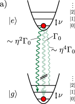
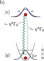
Figure 1: (a) $\Gamma_{\text{eff}}\ll\nu$: The two atoms prepared in the internal excited state $\ket{e}$ and the internal ground state $\ket{g}$ feel the same external harmonic oscillator potential. In the Lamb-Dicke limit ($\eta\ll 1$), the dominant decay channel for a single particle $\ket{e}\ket{0}\rightarrow\ket{g}\ket{0}$ with a rate $\Gamma_{0}$ is now blocked by the ground state atom due to the Pauli exclusion principle. The excited atom decays under change of its motional state with a rate $\Gamma_{\text{eff}}$ that is reduced of order $\eta^{2}$. (b) $\Gamma_{\text{eff}}\gg\nu$: In this scenario, the notion of motional eigenstates is meaningless for atoms in $\ket{e}$. Yet again, both atoms can be prepared in the same initial motional state represented by the wavepacket $\ket{0}$ (solid line). Dispersion of the motional wavepacket for the excited atom (dashed line) is slow compared to the effective decay dynamics. As before, the dominant decay channel is blocked and the effective decay rate is reduced of order $\eta^{2}$.

In this section, we first give a qualitative description of the effect of Pauli-blocked spontaneous emission in optical lattices and subsequently outline possible experimental realizations using alkali and alkaline-earth atoms.

Let us consider a three dimensional optical lattice that is loaded with two identical fermionic atoms per site and which is sufficiently deep that tunneling between neighboring sites is negligible on experimental timescales. Let us further assume that on each site one of the atoms is in an electronically excited state $\ket{e}$ while the other resides in its internal ground state $\ket{g}$. Due to its coupling to the electromagnetic field, the excited atom can undergo radiative decay. As a result of the Pauli exclusion principle, the presence of the ground state atom reduces the number of available decay channels, prolonging the lifetime of the excited state. For this blocking effect to be significant we require that both atoms are initially prepared in the same motional state, that the atoms are tightly confined to a region smaller than the optical wavelength of the electronic transition (Lamb-Dicke regime) and that decay from the excited state $\ket{e}$ is only possible to the internal ground state $\ket{g}$ (see Fig. 1(a)).

In the regime without tunneling the spatial potential on each lattice site is well approximated by a three dimensional harmonic oscillator potential. Here, for simplicity of this qualitative discussion, we regard motional excitations only in one dimension where the oscillator trapping frequency is $\nu$ and the vibrational eigenstates are denoted $\ket{n}$ ($n=0,1,\ldots$). This will later be extended to a 3D model. Furthermore, we assume for the moment that atoms in the internal excited state feel the same oscillator potential as ground state atoms, and that the natural linewidth $\Gamma$ of the state $\ket{e}$ is small compared to $\nu$. While these requirements simplify the discussion they are not mandatory, as we will argue below. For our initial state of interest, which is denoted $\ket{\psi_{0}}=c_{g0}^{\dagger}c_{e0}^{\dagger}\ket{\operatorname{vac}}$ in second quantized notation, both atoms reside in the motional ground state $\ket{0}$ and one is internally excited (see Fig. 1(a)). Here, $c^{\dagger}_{gn}$ ($c^{\dagger}_{en}$) creates a particle on the site we consider in the electronic state $\ket{g}$ ($\ket{e}$) and motional state $\ket{n}$. Treating the system within a Weisskopf-Wigner approximation Louisell (1973), the initial state $\ket{\psi_{0}}$ couples to the possible final atomic states $c_{g0}^{\dagger}c_{gn}^{\dagger}\ket{\operatorname{vac}}$ under emission of a one-photon wavepacket. The resulting dynamics within this ansatz yields an exponential decay for the population in the excited state with an effective decay rate

$$\Gamma_{\text{eff}}=\Gamma\sum_{n\neq 0}\int_{-1}^{1}\mathrm{d}u\,N(u)\lvert\braket{n}{\mathrm{e}^{-\mathrm{i}u\eta(a+a^{\dagger})}}{0}\rvert^{2}.$$ (1)

In Eq. (1), $\Gamma=d_{eg}^{2}\omega_{0}^{3}/(3\pi\varepsilon_{0}\hbar c^{3})$ is the usual single particle decay rate from $\ket{e}$ to $\ket{g}$ where $d_{eg}$ and $\omega_{0}$ are the dipole matrix element and frequency of the optical transition, respectively; $a^{\dagger}$ ($a$) denotes the creation (annihilation) operator for the harmonic oscillator and $N(u)$ is the angular distribution of dipole radiation projected onto the oscillator axis. The parameter $\eta=2\pi x_{0}/\lambda_{0}$ is given by the ratio between the oscillator ground state length $x_{0}=\sqrt{\hbar/(2M\nu)}$ with atomic mass $M$ and the wavelength of the emitted light $\lambda_{0}=2\pi c/\omega_{0}$. Note that in the sum over the final vibrational modes for the decaying atom, the mode $n=0$ is excluded due to the fermionic property $c_{g0}^{\dagger}c_{g0}^{\dagger}=0$, which reflects the Pauli-blocking of this particular channel.

In the Lamb-Dicke regime $x_{0}\ll\lambda_{0}$ the exponential in Eq. (1) can be expanded in the small parameter $\eta\ll 1$. In this limit, the leading contribution results from decay into the vibrational mode $n=1$, yielding an effective decay rate $\Gamma_{\text{eff}}\sim\eta^{2}\Gamma$. In contrast, a single particle decays at a total rate $\Gamma$. For two atoms, the excited state’s decay rate is decreased by a factor of order $\eta^{2}$. This results from blocking of the dominant decay channel, which corresponds to a decay while preserving the motional state, due to Pauli’s exclusion principle.

Let us now mention details and additional effects that modify the simplified picture outlined so far. Coming back to the preparation of the initial state $c_{g0}^{\dagger}c_{e0}^{\dagger}\ket{\operatorname{vac}}$, we distinguish the two scenarios $\Gamma_{\text{eff}}\ll\nu$ and $\Gamma_{\text{eff}}\gg\nu$. For $\Gamma_{\text{eff}}\ll\nu$ (see Fig. 1(a)) the decay is slow compared to the atomic motion. Such a situation can be realized by using metastable excited states of alkaline-earth atoms, where it is also possible to produce equal trapping potentials for ground state and excited atoms via magic wavelength lattices Katori et al. (2003); Ye et al. (2008). In this sideband resolved regime it is possible to laser-excite one of the atoms while exclusively coupling to the motional ground state. The opposite regime $\Gamma_{\text{eff}}\gg\nu$ (see Fig. 1(b)) is naturally realized for short-lived low-lying excited states in alkali atoms. Here, laser excitation from $\ket{g}$ to $\ket{e}$ is performed in the strong-excitation regime Poyatos et al. (1996) where the initial motional wavepacket remains essentially unchanged during the electronic transition and corresponds to the motional ground state for atoms in the internal state $\ket{g}$. In this regime a possibly different (anti-) trapping potential for excited state atoms gives rise only to a small correction to the Pauli-blocked decay dynamics. In this way, it is possible to initially prepare the ground and excited atom in the same motional state for either scenario, which will therefore lead to an effective decay rate $\Gamma_{\text{eff}}\sim\eta^{2}\Gamma$ in either case.

Furthermore, additional two-body effects appear, which will be taken into account in a more accurate treatment based on a second quantized many particle master equation (Section III). Since both atoms are confined to a region much smaller than $\lambda_{0}$, their mutual coupling to the radiation field gives rise to dipole-dipole interaction between the two atoms. In addition, cross-damping processes, which in other contexts are also responsible for super- and subradiance, can modify the decay characteristics. These effects are more often encountered in the limit $\Gamma\gg\nu$. Additionally, the influence of state changing collisions between the atoms will be addressed.

In the following two subsections we give an overview of possible realizations of Pauli-blocked spontaneous emission with ultracold atoms in optical lattices using (A) alkaline earth atoms and (B) alkali atoms. We will discuss the experimental requirements and steps for each scenario and show how the electronic dynamics of such multi-level atoms can be related to the effective two-level scheme discussed above.

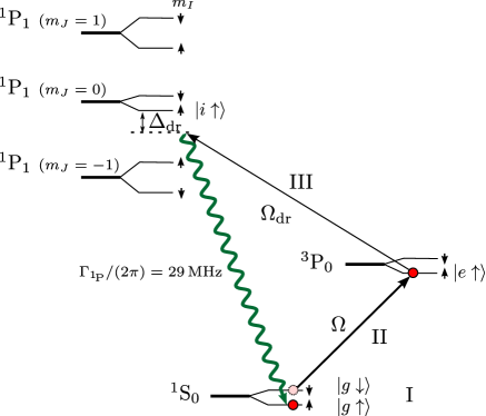
Figure 2: Relevant level structure (not to scale) and experimental sequence for alkaline earth-like atoms ([171]Yb in this example). (I) Two atoms per lattice site are prepared in $\ket{g\uparrow}$ and $\ket{g\downarrow}$, respectively; (II) one atom is excited from $\ket{g\downarrow}$ to the metastable state $\ket{e\uparrow}$ under a flip of its nuclear spin; (III) spontaneous emission from $\ket{e\uparrow}$ is induced by admixing the fast decaying state $\ket{i\uparrow}$. Nuclear spin flips during the induced decay are suppressed by applying a large external magnetic field which decouples nuclear and electronic spin in the ¹P₁ manifold. Consequently the induced decay from $\ket{e\uparrow}$ to $\ket{g\uparrow}$ is Pauli-blocked.

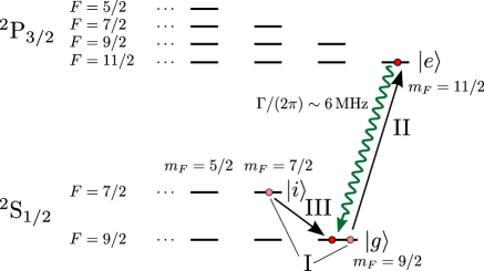
Figure 3: Relevant level structure (not to scale) and experimental sequence for alkali atoms ([40]K in this example). (I) Two atoms per lattice site are prepared in $\ket{g}$ and $\ket{i}$, respectively; (II) first, one atom is excited from $\ket{g}$ to the excited state $\ket{e}$; (III) then the other atom is transferred from $\ket{i}$ to $\ket{g}$. This pulse sequence is fast on the timescale given by $\Gamma^{-1}$. Choosing states with maximal $m_{F}$ values ensures that $\ket{g}$ and $\ket{e}$ form a closed two-level system. The decay of the excited atom back to $\ket{g}$ is Pauli-blocked.

II.1 Alkaline earth atoms

Alkaline earth atoms with two valence electrons offer the opportunity to demonstrate the effect of Pauli-blocked spontaneous emission in a way that is closely related to the qualitative model outlined above. These atoms have singlet ground states and metastable triplet states with lifetimes on the order of several tens of seconds. Since this exceeds accessible experimental timescales, we will use such a state as the excited state in our scheme and induce spontaneous emission by weak laser coupling to an intermediate state which rapidly decays to the internal ground state. Hence, the effective tunable decay rate can be made significantly larger than the natural linewidth of the metastable state. By operating the optical lattice at the “magic” wavelength it is possible to have equal trapping potentials for the ground and metastable excited state Katori et al. (2003); Ye et al. (2008). Furthermore, the fermionic isotopes have an additional nuclear spin degree of freedom, which we will make use of in the context of initial state preparation.

The relevant electronic level structure and experimental sequence I through III is illustrated in Fig. 2. (I) After the lattice is adiabatically ramped up on an ultracold cloud of atoms, two atoms per lattice site with the nuclear spin projections $\ket{\uparrow}$ and $\ket{\downarrow}$ reside in their motional and internal ground state $\ket{g}\ket{0}$ forming a band insulator. (II) With a $\pi$ pulse on the weakly dipole-allowed transition $\ket{g}\rightarrow\ket{e}$, one of the atoms is transferred from $\ket{g\downarrow}\ket{0}$ to the excited state $\ket{e\uparrow}\ket{0}$ while flipping its nuclear spin. (III) Finally, spontaneous emission from $\ket{e}$ is induced by admixing a fast decaying intermediate state. In order to avoid that the excited atom decays via the channel $\ket{e\uparrow}\rightarrow\ket{g\downarrow}$ which is not Pauli-blocked, one can either use a sufficiently large external magnetic field Reichenbach and Deutsch (2007), or alternatively choose an appropriate polarization of the dressing laser. For both cases this leads to a decoupling of electronic and nuclear spin for the induced decay process (see Fig. 2), and as the intermediate state is only virtually populated, $\ket{e\uparrow}$ and $\ket{g\uparrow}$ form a closed system regarding the internal degrees of freedom.

As a consequence the described system constitutes a realization of the model system illustrated in Fig. 1(a) where the excited atom can only undergo decay under change of its motional state. The induced decay rate is by a factor of order $\eta^{2}$ smaller than it is for a single atom.

II.2 Alkali atoms

In contrast to the alkaline earth case, alkali atoms have one valence electron whose lower excited states decay to the ground state on dipole-allowed transitions with a large linewidth $\Gamma$ on the order of several $\mathrm{MHz}$.

In Fig. 3 a typical alkali level structure and a possible experimental scheme is shown. We choose to make use of the transition between the hyperfine sublevels $\ket{e}$ and $\ket{g}$ with maximal $m_{F}$ values, because the only dipole-allowed transition for atoms prepared in $\ket{e}$ is decay to $\ket{g}$, so these states form an effective closed two-level system. (I) The lattice is prepared with two atoms per lattice site in the ground state sublevels $\ket{i}$ and $\ket{g}$ (both in their motional ground state $\ket{0}$). (II) The first atom is excited with a state selective $\pi$ pulse from $\ket{g}$ to $\ket{e}$. (III) The second atom is transferred from $\ket{i}$ to $\ket{g}$ with a radio frequency or Raman $\pi$ pulse. The total pulse sequence should be fast compared to the timescale $\Gamma^{-1}$ so that spontaneous emission during the preparation sequence can be neglected. The excited atom then undergoes radiative decay with a Pauli-blocked rate on the order of $\eta^{2}\Gamma$.

As a consequence of the large linewidth $\Gamma$ imperfections are introduced that will qualitatively modify the Pauli-blocking effect: (i) the induced dipole-dipole interaction between atoms is strong for large $\Gamma$ and will excite motional states that are not blocked; (ii) due to the fast excitation pulses the transfer to $\ket{e}$ is performed in the strong-excitation regime where the Rabi frequency is much larger than the oscillator spacing $\nu$ of the ground state. Thus, the initial motional state $\ket{0}$ is displaced by the momentum recoil of the absorbed photon. This leads to slightly different motional states for the ground and excited state atom; (iii) in general, the atoms encounter different (anti-)trapping potentials for their internal ground and excited states. However, due to the large separation of timescales $\nu\ll\Gamma$, corrections to the dynamics due to atomic motion during the decay are small. All these effects will be discussed in more detail in the following section.

III Analysis and Results

In this section we first discuss the many-body master equation for fermionic two-level atoms in second quantization. We show how Pauli-blocking emerges naturally in this description and discuss collective effects which arise for more than one atom. Subsequently, we present a detailed quantitative discussion of the experimental realizations with both alkaline earth-like and alkali atoms.

III.1 Master equation

We consider fermionic two-level atoms with internal states $\ket{e}$ and $\ket{g}$ separated by the energy $\hbar\omega_{0}=\hbar ck_{0}$ and coupled to the radiation field acting as a bath. The center of mass motion of the atoms takes place in a three dimensional harmonic oscillator potential with trapping frequencies $\bm{\nu}=(\nu_{1},\nu_{2},\nu_{3})$ for the three spatial dimensions and eigenstates $\ket{\bm{n}}=\ket{n_{1}}\ket{n_{2}}\ket{n_{3}}$ ($n_{j}=0,1,\cdots$) on each lattice site for a deep optical lattice with strongly suppressed tunneling. We are interested in a situation where the atoms are confined to a region small compared to the optical wavelength $\lambda_{0}=2\pi/k_{0}$. Under assumption of the Born-Markov approximation, the dynamics is described by a standard quantum optical master equation Lehmberg (1970); Kazantsev et al. (1990); Pichler et al. (2010)

$$\dot{\rho}=-\frac{\mathrm{i}}{\hbar}(H_{\text{eff}}\rho-\rho H_{\text{eff}}^{\dagger})+\hat{\Gamma}[\rho],$$ (2)

where for our purposes we explicitly take into account the indistinguishability and the motional degrees of freedom of the atoms. The terms appearing in the effective non-hermitian Hamiltonian $H_{\text{eff}}$ and in the recycling term $\hat{\Gamma}[\rho]$ are discussed in this subsection.

The effective Hamiltonian can be written as the sum of a hermitian and a non-hermitian part, $H_{\text{eff}}=H_{\text{eff}}^{(0)}+H_{\text{eff}}^{(1)}$. In

$$H_{\text{eff}}^{(0)} = \smashoperator[]{\sum_{\bm{n}}^{}}\hbar\bm{\nu}\cdot\bm{n}\,\left(c_{g\bm{n}}^{\dagger}c_{g\bm{n}}+c_{e\bm{n}}^{\dagger}c_{e\bm{n}}\right)$$ (3)

$$-\smashoperator[]{\sum_{\bm{m}\bm{n}\bm{m}^{\prime}\bm{n}^{\prime}}^{}}\hbar L_{\bm{n}^{\prime}\bm{m}^{\prime}\bm{m}\bm{n}}c_{e\bm{n}^{\prime}}^{\dagger}c_{g\bm{m}^{\prime}}^{\dagger}c_{g\bm{m}}c_{e\bm{n}}$$

the first term accounts for the motion of the atoms in the harmonic oscillator potential. Here $c_{\beta\bm{n}}$ ($c_{\beta\bm{n}}^{\dagger}$) are the annihilation (creation) operators for an atom in the internal state $\beta\in\left\{e,g\right\}$ and in the vibrational mode $\ket{\bm{n}}$ of the harmonic oscillator. These operators obey the fermionic anti-commutation relations $\{c_{\beta\bm{n}}^{\dagger},c_{\beta^{\prime}\bm{n}^{\prime}}^{\dagger}\}=\{c_{\beta\bm{n}},c_{\beta^{\prime}\bm{n}^{\prime}}\}=0$ and $\{c_{\beta\bm{n}}^{\dagger},c_{\beta^{\prime}\bm{n}^{\prime}}\}=\delta_{\beta,\beta^{\prime}}\delta_{\bm{n},\bm{n}^{\prime}}$. The second term in Eq. (3), a two particle operator, is the dipole-dipole interaction between the atoms, which is induced by the collective coupling to the radiation field and has to be taken into account when the distance between the atoms is comparable to or smaller than $\lambda_{0}$. It is given by

$$L_{\bm{n}^{\prime},\bm{m}^{\prime},\bm{m},\bm{n}} = \Gamma\smashoperator[]{\iint_{}^{}}\mathrm{d}^{3}x\,\mathrm{d}^{3}x^{\prime}\,G(k_{0}(\bm{x}-\bm{x}^{\prime}))$$ (4)

$$\times\varphi_{\bm{n}^{\prime}}(\bm{x})\varphi_{\bm{m}^{\prime}}(\bm{x}^{\prime})\varphi_{\bm{m}}(\bm{x})\varphi_{\bm{n}}(\bm{x}^{\prime})$$

$$G(\bm{\xi}) = \frac{3}{4}\frac{1-3(\hat{\bm{d}}_{eg}\cdot\hat{\bm{\xi}})^{2}}{\xi^{3}},$$ (5)

where $\Gamma$ is the single particle decay rate from $\ket{e}$ to $\ket{g}$ as defined above, $\varphi_{\bm{m}}(\bm{x})$ are the position space harmonic oscillator eigenfunctions and $\hat{\bm{d}}_{eg}$ denotes the dipole matrix element unit vector of the transition. The representation Eq. (5) for the function $G(\bm{\xi})$ is valid in the limit $\lvert\xi\rvert\ll 1$ which is fulfilled in the Lamb-Dicke regime. For broader traps with interatomic distances $k_{0}\lvert\bm{x}-\bm{x}^{\prime}\rvert\sim 1$ there are corrections to $G(\bm{\xi})$ of order $1/\xi^{2}$ Lehmberg (1970).

The non-hermitian part of the effective Hamiltonian reads

$$H_{\text{eff}}^{(1)} = -\frac{\mathrm{i}}{2}\hbar\Gamma\sum_{\bm{n}}c_{e\bm{n}}^{\dagger}c_{e\bm{n}}$$ (6)

$$+\frac{\mathrm{i}}{2}\hbar\Gamma\smashoperator[]{\sum_{\bm{m}\bm{n}\bm{m}^{\prime}\bm{n}^{\prime}}^{}}\tilde{R}_{\bm{n}^{\prime}\bm{m}\bm{m}^{\prime}\bm{n}}c_{e\bm{n}^{\prime}}^{\dagger}c_{g\bm{m}^{\prime}}^{\dagger}c_{g\bm{m}}c_{e\bm{n}}$$

$$\tilde{R}_{\bm{n}^{\prime}\bm{m}\bm{m}^{\prime}\bm{n}} = \int\mathrm{d}\Omega_{\hat{\bm{k}}}\,N(\hat{\bm{k}})R^{\ast}_{\bm{n}^{\prime}\bm{m}}(\hat{\bm{k}})R_{\bm{m}^{\prime}\bm{n}}(\hat{\bm{k}}),$$ (7)

where

$$N(\hat{\bm{k}})=\frac{3}{8\pi}\left(1-\lvert\hat{\bm{d}}_{eg}\cdot\hat{\bm{k}}\rvert^{2}\right)$$

is the angular distribution of dipole radiation, $\hat{\bm{k}}=(\hat{k}_{1},\hat{k}_{2},\hat{k}_{3})$ denotes the unit vector of the photon emission direction, $R_{\bm{m}\bm{n}}(\hat{\bm{k}})\equiv\prod_{j=1,2,3}R_{m_{j}n_{j}}(\hat{k}_{j})=\prod_{j}\braket{m_{j}}{\mathrm{e}^{-\mathrm{i}\hat{k}_{j}\eta_{j}(a_{j}+a_{j}^{\dagger})}}{n_{j}}$ the recoil matrix elements (see Appendix A), $\eta_{j}=k_{0}\sqrt{\hbar/(2M\nu_{j})}$ the Lamb-Dicke parameter corresponding to the $j$-axis, and $a_{j}$ ($a_{j}^{\dagger}$) the annihilation (creation) operators for vibrational excitations along the $j$-axis. The effective Hamiltonian Eq. (3) and (6) is valid under the assumption that the system size is small compared to the distance which light travels on typical timescales of the system dynamics. This is always fulfilled for optical transitions and a system size on the order of an optical wavelength.

The recycling term is given by

$$\hat{\Gamma}[\rho] = \Gamma\smashoperator[]{\sum_{\bm{m}\bm{n}\bm{m}^{\prime}\bm{n}^{\prime}}^{}}\tilde{R}_{\bm{n}^{\prime}\bm{m}^{\prime}\bm{m}\bm{n}}c_{g\bm{m}}^{\dagger}c_{e\bm{n}}\rho c_{e\bm{n}^{\prime}}^{\dagger}c_{g\bm{m}^{\prime}}$$ (8)

The coefficients $\tilde{R}_{\bm{n}^{\prime}\bm{m}^{\prime}\bm{m}\bm{n}}$ account for the momentum recoil of the emitted photon during a quantum jump.

For our initial state of interest with two atoms, both residing in the ground state of the three dimensional harmonic oscillator and one being internally excited, the density operator is given by $\rho_{0}=c_{g\bm{0}}^{\dagger}c_{e\bm{0}}^{\dagger}\ket{\operatorname{vac}}\bra{\operatorname{vac}}c_{e\bm{0}}c_{g\bm{0}}$. In the recycling term for this initial state $\hat{\Gamma}[\rho_{0}]$, quantum jump terms that correspond to a decay of the excited atom while remaining in the ground state of the harmonic oscillator (i.e. terms with $\bm{m}=\bm{0}$, $\bm{m}^{\prime}=\bm{0}$) are identically zero due to the fermionic properties $c_{g\bm{0}}^{\dagger}c_{g\bm{0}}^{\dagger}=c_{g\bm{0}}c_{g\bm{0}}=0$, reflecting the Pauli-blocking of this particular channel. The total initial decay rate $\Gamma_{\text{eff}}$ of the excited atom is given by the sum over all available decay channels

$$\Gamma_{\text{eff}} =\smashoperator[]{\sum_{\bm{m}\neq\bm{0}}^{}}\braket{g\bm{0};g\bm{m}}{\hat{\Gamma}[\rho_{0}]}{g\bm{0};g\bm{m}}$$

$$=\Gamma\int\mathrm{d}\Omega_{\hat{\bm{k}}}\,N(\hat{\bm{k}})\smashoperator[]{\sum_{\bm{m}\neq\bm{0}}^{}}\lvert R_{\bm{m}\bm{0}}(\hat{\bm{k}})\rvert^{2},$$ (9)

where $\ket{g\bm{0};g\bm{m}}=c_{g\bm{0}}^{\dagger}c_{g\bm{m}}^{\dagger}\ket{\operatorname{vac}}$. Equation (9) is the generalization of Eq. (1) to a 3D setup. In the Lamb-Dicke limit $\eta_{j}\ll 1$, to second order in $\eta_{j}$ only decay to the three oscillator states with one motional quantum ($\ket{g\bm{0};g\bm{m}}$ with $\lvert m\rvert=1$) contributes to $\Gamma_{\text{eff}}$. Expanding the recoil matrix elements in the small parameters $\eta_{j}$ yields $\lvert R_{10}(\hat{\bm{k}})\rvert^{2}=\hat{k}_{j}^{2}\eta_{j}^{2}+\mathcal{O}(\eta_{j}^{4})$ for the $j$-axis. The total initial decay rate in this limit is $\Gamma_{\text{eff}}=\sum_{j=1,2,3}\alpha_{j}\eta_{j}^{2}\Gamma+\mathcal{O}(\eta_{j}^{4})$, where $\alpha_{j}$ are numerical coefficients of order $1$ and depend on the relative orientation of the transition dipole matrix element to the $j$-axis. More details on these coefficients and on $\Gamma_{\text{eff}}$ beyond the Lamb-Dicke limit can be found in appendix A. For the special case of an isotropic harmonic oscillator (i.e. $\nu_{1}=\nu_{2}=\nu_{3}$) the particularly simple result $\Gamma_{\text{eff}}=\eta^{2}\Gamma+\mathcal{O}(\eta^{4})$ is found.

Let us now return to the discussion of the collective effects introduced by the dipole-dipole interaction (Eq. (4)) and the cross-damping terms (Eq. (6)), still concentrating on the case of two atoms trapped in the Lamb-Dicke regime. The dipole-dipole interaction couples different vibrational levels of two-particle states where one atom is internally excited and the other is in its internal ground state. In evaluating the matrix elements in Eq. (4), divergences at short relative distances appear, which reflect the fact that, in principle, one would have to solve the exact two-atom problem to capture the right behaviour. Effects of the short-range potential are important at distances comparable to a few tens of Bohr radii Pichler et al. (2010). However, in order to estimate the order of magnitude for the leading terms it is sufficient to treat the atoms as independent particles being described by their internal state and center of mass wavefunction. The divergence of the dipole-dipole matrix elements can then be avoided in a standard way by introducing a spatial cutoff for the relative distance between the atoms, which yields a finite result independent of the cutoff. By this procedure, the leading terms of the dipole-dipole matrix elements are found to be on the order of $\Gamma/(100\eta^{3})$. Note that the classical scaling of the dipole-dipole interaction with the inverse distance cubed is reflected in the $\eta$ dependence. Another process in this case leading to dissipative redistribution between excited oscillator states are non-diagonal cross-damping terms contained in the non-hermitian Hamiltonian Eq. (6). The leading terms are of order $\eta^{2}\Gamma$.

In the case of an experimental realization with alkali atoms where the linewidth $\Gamma$ is large, the dipole-dipole interaction is the dominant source of imperfections and competes with the Pauli-blocking effect as it couples the motional state $\rho_{0}$ to motional states that are not blocked. A compromise has to be found for $\eta$: smaller values of $\eta$ lead to a larger blocking effect, but also to a larger dipole-dipole interaction. When estimating the rate at which the system leaves the initial Pauli-blocked state due to dipole-dipole interaction one must take care of divergences in the sum over all intermediate states. In situations where this rate is on the order of the original $\Gamma$ even for large $\eta$, the Pauli-blocking of spontaneous emissions would no longer be observable because the atoms will be transferred to a configuration of motional states that is unblocked on timescales comparable to the original spontaneous emission rate.

In contrast, for an implementation with alkaline-earth atoms the small natural linewidth of the metastable excited state makes the dipole-dipole interaction and the cross-damping processes negligible. Additionally, as will be argued in the next subsection, the impact of these effects on the spontaneous emission process which is induced by admixing an excited state with a large decay rate can be avoided by coupling far off-resonantly to this intermediate state.

III.2 Alkaline earth-like atoms

In this subsection we further elaborate on the experimental realization of Pauli-blocked spontaneous emission with alkaline earth-like atoms, commenting in more detail on the initial state preparation in a “magic” wavelength optical lattice, quenching of the metastable excited state to induce spontaneous emission and the application of an external magnetic field to decouple the nuclear and electronic spin degrees of freedom. To be specific we present the experimental scheme choosing the isotope [171]Yb, which due to its nuclear spin $I=1/2$ exhibits a particularly simple level structure. The discussion, though, can be readily adapted to other fermionic alkaline earth(-like) species, such as [87]Sr.

In Fig. 2 the relevant electronic states and experimental steps are illustrated. The doubly forbidden “clock” transition $(6s^{2})^{1}\text{S}_{0}\leftrightarrow(6s6p)^{3}\text{P}_{0}$ is weakly dipole-allowed due to hyperfine mixing with higher lying P-states and has a natural linewidth $\gamma/(2\pi)\sim$10\text{\,}\mathrm{mHz}$$ Boyd et al. (2007); Porsev et al. (2004). The nuclear spin decouples from the electronic degrees of freedom for the ground state with total electronic angular momentum $J=0$, and the two magnetic sublevels are given by $\ket{{}^{1}\text{S}_{0};m_{I}=\pm 1/2}$. For the metastable excited state ³P₀ the total angular momentum projection $m_{F}$ rather than the nuclear spin projection $m_{I}$ is a good quantum number due to the small hyperfine admixture of electronic angular momentum. Nevertheless, the magnetic sublevels are still almost pure $m_{I}$ eigenstates. The states with $m_{I}=\pm 1/2$ are denoted as $\ket{\uparrow}$ and $\ket{\downarrow}$, respectively.

We choose the ground state $\ket{g\uparrow}=\ket{{}^{1}\text{S}_{0};m_{I}=1/2}$ and the metastable excited state $\ket{e\uparrow}=\ket{{}^{3}\text{P}_{0};m_{I}=1/2}$ as the starting point from which the Pauli-blocking effect can be observed (see Fig. 1(a)), since the tiny natural linewidth $\gamma$ of the “clock” transition renders both direct radiative decay and dipole-dipole interaction between these two states negligible.

The requirement of equal trapping potentials for the states $\ket{e\uparrow}$ and $\ket{g\uparrow}$ can be met by operating the optical lattice at the “magic” wavelength of $759\text{\,}\mathrm{nm}$ Porsev et al. (2004); Kohno et al. (2009). At this wavelength, the AC polarizability and, thus, the light shift caused by the lattice laser is the same for the ¹S₀ and the ³P₀ state to first order in the laser intensity. In the regime of a deep optical lattice where tunneling between the sites is negligible, the spatial potential on each lattice site is well approximated by a 3D harmonic oscillator with trapping frequencies $\bm{\nu}$. Vibrational frequencies of $\nu/(2\pi)=$90\text{\,}\mathrm{kHz}$$ have already been realized in a 1D optical lattice (Barber et al., 2006).

Let us now turn to the discussion of state preparation and the required sequence of laser pulses.

(I) Loading of the optical lattice with two atoms per site can be achieved by adiabatically ramping up the lattice potential on a cloud of ultracold atoms Viverit et al. (2004); Köhl et al. (2005). For a temperature lower than the motional level spacing, a band insulator with two atoms per lattice site in the motional ground state $\ket{\bm{0}}$ and with opposite nuclear spin projections $\ket{\uparrow}$ and $\ket{\downarrow}$ will form. The resulting state on each lattice site is $c_{g\uparrow\bm{0}}^{\dagger}c_{g\downarrow\bm{0}}^{\dagger}\ket{\operatorname{vac}}$ (see Fig. 2 I).

(II) To prepare a suitable initial state in order to observe Pauli-blocking, the atom in $\ket{g\downarrow}\ket{\bm{0}}$ is excited with a laser $\pi$-pulse on the “clock” transition with Rabi frequency $\Omega$. Recoil-free excitation is possible in the easily accessible regime $\nu_{\text{max}}\gg\Omega\gg\gamma$ where most conveniently the laser direction is chosen along the axis of strongest confinement. In this limit, spontaneous emission can be neglected and the vibrational sidebands are well resolved. Choosing $\sigma^{+}$ polarized light flips the nuclear spin due to hyperfine interaction and furthermore ensures that the other atom is not affected by the pulse. By tuning the laser on the carrier transition, the initial state of interest $c_{g\uparrow\bm{0}}^{\dagger}c_{e\uparrow\bm{0}}^{\dagger}\ket{\operatorname{vac}}$ is prepared.

(III) Quenching the excited state offers the possibility to induce a tunable effective decay rate from $\ket{e\uparrow}$ to $\ket{g\uparrow}$ that exceeds the natural linewidth $\gamma$, and also to produce a decay that will not flip the nuclear spin state (which is not the case for intrinsic decay of the ³P₀ manifold, as the transition is weakly allowed due to hyperfine coupling). A dressing laser couples the metastable excited state $\ket{e\uparrow}$ on the weakly magnetic dipole-allowed transition to the intermediate state $(6s6p)^{1}\text{P}_{1}$ Santra et al. (2005), which has a large linewidth $\Gamma_{{}^{1}\!\text{P}}/(2\pi)=$29\text{\,}\mathrm{MHz}$$. Decay from ¹P₁ to states other than the ¹S₀ ground state occurs with a negligible probability.

One has to ensure that during the decay induced by this dressing the nuclear spin of the initially excited atom is not flipped due to hyperfine interaction, as the decay channel $\ket{e\uparrow}\rightarrow\ket{g\downarrow}$ is not Pauli-blocked. This can be achieved by dressing $\ket{e\uparrow}$ with a state in the ¹P₁ manifold that only contains the $\ket{\uparrow}$ component, i.e. a product state of the form $\ket{m_{J};m_{I}=1/2}$. The only decay channel for such a state is into $\ket{g\uparrow}$ as follows from the selection rule $\Delta m_{I}=0$ for electric dipole transitions. In the following we will discuss how such coupling to an $\ket{\uparrow}$ state can be accomplished by either (i) using $\sigma^{+}$ polarized dressing light to couple $\ket{e\uparrow}$ exclusively to the magnetic sublevel with maximal $m_{F}$ which is a $m_{I}=1/2$ eigenstate, or alternatively (ii) using $\pi$ or $\sigma^{-}$ polarized dressing light while decoupling nuclear and electronic spin in the ¹P₁ manifold with an external magnetic field in the Paschen-Back regime Reichenbach and Deutsch (2007). To this end we diagonalize the Hamiltonian governing the ¹P₁ subspace including hyperfine- and Zeeman interaction

$$\hat{H}=A\hat{\bm{\mathrm{I}}}\cdot\hat{\bm{\mathrm{J}}}/\hbar^{2}+g_{j}\mu_{B}\hat{\bm{\mathrm{J}}}\cdot\bm{B}/\hbar-g_{I}\mu_{N}\hat{\bm{\mathrm{I}}}\cdot\bm{B}/\hbar.$$ (10)

Here $g_{J}$ Baumann and Wandel (1968) and $g_{I}$ Olschewski and Otten (1967) are the electron and nuclear $g$ factors, $A$ Berends and Maleki (1992) is the magnetic hyperfine constant and $\bm{B}$ an external magnetic field.

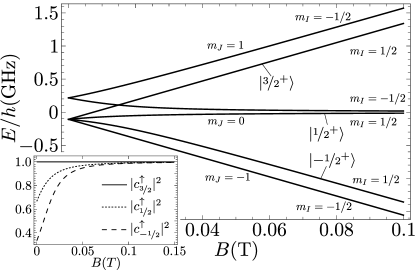
Figure 4: Zeeman diagram of the ¹P₁ manifold. The eigenstates approach product states of electronic and nuclear spin for a large magnetic field. The states suitable for dressing the metastable excited state $\ket{e\uparrow}$ without flipping the nuclear spin during the decay are $\ket{m_{F}^{+}}$ with $m_{F}=3/2,1/2,-1/2$. In the inset, the probability for decaying without nuclear spin flip is plotted as a function of the external magnetic field.

The eigenstates, which are denoted $\ket{m_{F}^{\pm}}$, approach product states of electronic and nuclear spin for large values of $B$ in the Paschen-Back regime $\mu_{B}B\gg A$ as illustrated in the Zeeman diagram in Fig. 4. The sign $\pm$ labels the nuclear spin projection in this limit, i.e. $\ket{m_{F}^{\pm}}\rightarrow\ket{m_{J}{=}m_{F}{\mp}1/2;m_{I}{=}{\pm}1/2}$. One can couple to the three states $\ket{m_{F}^{+}}$ with $m_{F}=3/2,1/2,-1/2$, which are suitable as intermediate states for the quenching process, with $\sigma^{+}$, $\pi$ and $\sigma^{-}$ polarized laser light, respectively. Their expansion in terms of product states $\ket{m_{j};m_{I}}$ is

$$\ket{m_{F}^{+}}=c_{m_{F}}^{\uparrow}\ket{m_{J}=m_{F}-1/2;m_{I}=1/2}\\ +c_{m_{F}}^{\downarrow}\ket{m_{J}=m_{F}+1/2;m_{I}=-1/2}.$$

The $B$-dependence of the coefficients is given by

$$c_{m_{F}}^{\uparrow(\downarrow)} =\left[\frac{1}{2}\left(1\mathbin{\vbox{\hbox{\oalign{\hfil${+}$\hfil\cr\kern-1.29167pt\cr$({-})$\cr}}}}\frac{x+\frac{2}{3}m_{F}}{\sqrt{x^{2}+\frac{4}{3}m_{F}x+1}}\right)\right]^{\frac{1}{2}},$$

where $x=2(g_{j}\mu_{B}+g_{I}\mu_{N})B/(3\lvert A\rvert)$ is a dimensionless variable for the magnetic field strength. The probability for decaying from $\ket{m_{F}^{+}}$ to $\ket{g\uparrow}$ or $\ket{g\downarrow}$ is $\lvert c_{m_{F}}^{\uparrow}\rvert^{2}$ and $\lvert c_{m_{F}}^{\downarrow}\rvert^{2}$, respectively (see inset Fig. 4). Note that (i) if one chooses to work with a $\sigma^{+}$ polarized dressing laser, a weak magnetic field defining the quantization axis is sufficient because $\lvert c_{3/2}^{\uparrow}\rvert^{2}$ is identically $1$ for arbitrary $B$-values, and $\sigma^{+}$ polarized light couples $\ket{e\uparrow}$ exclusively to $\ket{3/2^{+}}$ in the ¹P₁ manifold. On the other hand, (ii) for $\pi$ and $\sigma^{-}$ polarized light the external magnetic field has to be sufficiently strong so that $\lvert c_{\pm 1/2}^{\uparrow}\rvert^{2}$ approaches unity and the Zeeman splitting becomes large enough so that coupling to $\ket{m_{F}^{-}}$ is negligible. For a magnetic field of $0.05\text{\,}\mathrm{T}$ the probability to decay without nuclear spin flip is $>$95\text{\,}\mathrm{\char 37\relax}$$. The arguments presented here for [171]Yb are also applicable to other alkaline earth-like species which may have a nuclear spin $I>1/2$. Method (i) requires that states with maximal or minimal $m_{I}$ and $m_{F}$ values are used in the protocol whereas method (ii) is suitable for arbitrary $m_{I}$ sublevels. The decoupling of nuclear and electronic spin in the limit of large $B$ also holds for isotopes with $I>1/2$ where additional quadrupole effects have to be taken into account in the Hamiltonian Eq. (10) Reichenbach and Deutsch (2007); Boyd et al. (2007).

After having discussed the required experimental steps let us turn to the resulting Pauli-blocked decay dynamics. First we show that this dynamics is described by a coupled set of effective rate equations for the populations in $\ket{e}$ and $\ket{g}$. Subsequently we provide a suitable set of experimental parameters.

We are interested in a regime where the detuning of the dressing laser $\Delta_{\text{dr}}$ is large compared to all the other characteristic frequencies which govern the system dynamics: the linewidth $\Gamma_{{}^{1}\!\text{P}}$, the dipole-dipole interaction for two atoms in ¹S₀ and ¹P₁, respectively, the dressing laser Rabi frequency $\Omega_{\text{dr}}$ and the trapping frequency $\nu$ of both the metastable excited and the ground state. Under these conditions the intermediate state is only virtually populated and can be adiabatically eliminated. Furthermore, in the resulting effective decay dynamics the ground state atom in $\ket{g\uparrow}\ket{\bm{0}}$ acts as a spectator not taking part in the dynamics but blocking the dominant decay channel $\ket{e\uparrow}\ket{\bm{0}}\rightarrow\ket{g\uparrow}\ket{\bm{0}}$ for the excited atom. The corresponding dynamics in the Lamb-Dicke limit and for the special case of an isotropic trap is described by the rate equations

$$\dot{P}_{e\uparrow} =-\left(\left|c_{m_{F}}^{\uparrow}\right|^{2}(\eta^{2}+\eta_{\text{dr}}^{2})+\left|c_{m_{F}}^{\downarrow}\right|^{2}\right)\Gamma P_{e\uparrow}+\mathcal{O}(\eta^{4})$$

$$\dot{P}_{g\uparrow} =\left|c_{m_{F}}^{\uparrow}\right|^{2}(\eta^{2}+\eta_{\text{dr}}^{2})\Gamma P_{e\uparrow}+\mathcal{O}(\eta^{4})$$

$$\dot{P}_{g\downarrow} =\lvert c_{m_{F}}^{\downarrow}\rvert^{2}\Gamma P_{e\uparrow}.$$

Here we have introduced the effective decay rate $\Gamma=\Omega_{\text{dr}}^{2}/(4\Delta_{\text{dr}}^{2})\Gamma_{{}^{1}\!\text{P}}$ and the populations of the reduced system density matrix

$$P_{e\uparrow} = \braket{\operatorname{vac}}{c_{e\uparrow\bm{0}}c_{g\uparrow\bm{0}}\rho c_{g\uparrow\bm{0}}^{\dagger}c_{e\uparrow\bm{0}}^{\dagger}}{\operatorname{vac}}$$

$$P_{g\uparrow} = \sum_{\bm{m}\neq\bm{0}}\braket{\operatorname{vac}}{c_{g\uparrow\bm{m}}c_{g\uparrow\bm{0}}\rho c_{g\uparrow\bm{0}}^{\dagger}c_{g\uparrow\bm{m}}^{\dagger}}{\operatorname{vac}}$$

$$P_{g\downarrow} = \sum_{\bm{m}}\braket{\operatorname{vac}}{c_{g\downarrow\bm{m}}c_{g\uparrow\bm{0}}\rho c_{g\uparrow\bm{0}}^{\dagger}c_{g\downarrow\bm{m}}^{\dagger}}{\operatorname{vac}}.$$

The latter describe the probability of finding the initially excited atom in $\ket{e\uparrow}$, $\ket{g\uparrow}$ and $\ket{g\downarrow}$, respectively, while the other atom remains in $\ket{g\uparrow}\ket{\bm{0}}$. The two Lamb-Dicke parameters $\eta$ and $\eta_{\text{dr}}$ correspond to the momentum recoils of the induced spontaneous emission and the dressing laser photon, respectively. The main result for the initial state $c_{g\uparrow\bm{0}}^{\dagger}c_{e\uparrow\bm{0}}^{\dagger}\ket{\operatorname{vac}}$ described by $P_{e\uparrow}=1$ and $P_{g\uparrow}=P_{g\downarrow}=0$ is a total decay rate from $\ket{e\uparrow}\ket{\bm{0}}$ given by $\Gamma_{\text{eff}}=(\lvert c_{m_{F}}^{\uparrow}\rvert^{2}(\eta^{2}+\eta_{\text{dr}}^{2})+\lvert c_{m_{F}}^{\downarrow}\rvert^{2})\Gamma$. In the regime of interest $\lvert c_{m_{F}}^{\uparrow}\rvert^{2}\rightarrow 1$ and $\lvert c_{m_{F}}^{\downarrow}\rvert^{2}\rightarrow 0$, the decay rate $\Gamma_{\text{eff}}$ is of order $\eta^{2}$ smaller than the effective induced decay rate $\Gamma$ from $\ket{e\uparrow}$ to $\ket{g\uparrow}$ for a single atom.

In this discussion so far we have not included elastic and inelastic collisions between the two atoms. Collisional shifts do not affect the experiment as long as they are small compared to the motional level spacing. State changing collisions can lead to loss of the atoms from the lattice. While, in principle, the collisional loss from two atoms in ³P₀ could be strong, this situation is never encountered in our protocol. Here, we only require the ¹S₀–³P₀ inelastic collisions to be small compared to the quenching rate in the experiment.

A suitable choice for the detuning $\Delta_{\text{dr}}$ is dictated by the requirement that this has to be the largest frequency scale in the dynamics and simultaneously a sufficiently large effective decay rate $\Gamma$ has to be induced for a given dressing laser Rabi frequency $\Omega_{\text{dr}}$. For [171]Yb with a typical trapping frequency $\nu/(2\pi)=$90\text{\,}\mathrm{kHz}$$, the Lamb-Dicke parameters $\eta=0.28$ and $\eta_{\text{dr}}=0.09$ correspond to transitions with wavelengths $\lambda=$399\text{\,}\mathrm{nm}$$ and $\lambda_{\text{dr}}=$1285\text{\,}\mathrm{nm}$$, respectively. The dipole-dipole interaction between two atoms in ¹S₀ and the virtually populated ¹P₀, respectively, can be estimated to be on the order of $\Gamma_{{}^{1}\!\text{P}}$ so that $\Delta_{\text{dr}}\gg\Gamma_{{}^{1}\!\text{P}}$ is required. For $\Delta_{\text{dr}}=10\Gamma_{{}^{1}\!\text{P}}$, with a Rabi frequency $\Omega_{\text{dr}}=$4\text{\,}\mathrm{MHz}$$, an effective decay rate of $\Gamma=$220\text{\,}\mathrm{Hz}$$ can be reached. Note that as an alternative to the direct coupling ³P₀$\leftrightarrow$¹P₀, quenching of the metastable excited state can be done via a two-photon Raman process involving the dipole-allowed transition ³P₀$\leftrightarrow$³S₁ and the intercombination transition ³S₁$\leftrightarrow$¹P₁ which can lead to a larger two-photon Rabi frequency $\Omega_{\text{dr}}$ Reichenbach and Deutsch (2007).

III.3 Alkali atoms

Let us now turn to alkali atoms with their fastly decaying low lying transitions (see Fig. 3). Here, both the laser excitation and the subsequent decay dynamics are fast compared to the motion of the atoms in the trap. In contrast to the alkaline earth case, where it is important to have equal trapping potentials for ground and excited state atoms, the notion of motional eigenstates becomes irrelevant for the spectrally very broad excited states in alkali atoms, therefore the optical potential for internally excited atoms does not play a crucial role in this scenario.

First we will analyze the experimental requirements and sequences to observe Pauli-blocked spontaneous emission using alkali atoms. Subsequently, we will discuss imperfections associated with the large linewidth of the considered transition and estimate their impact.

The relevant level scheme and the sequence of laser pulses is sketched in Fig. 3 for [40]K as a representative of the alkali family, though the scheme presented here is not specific to a particular species and can readily be adapted to other fermionic alkali isotopes. We propose to use the magnetic sublevels with maximal projection of total angular momentum $m_{F}$, i.e. $\ket{g}=\ket{{}^{2}\text{S}_{1/2};F=9/2;m_{F}=9/2}$ and $\ket{e}=\ket{{}^{2}\text{P}_{3/2};F=11/2;m_{F}=11/2}$, as ground and excited states as depicted in Fig. 1(b). For atoms in the internal state $\ket{e}$, the decay to $\ket{g}$ is the only dipole-allowed transition, ensuring that these states form a closed effective two-level system regarding spontaneous emission. To prepare an initial state suitable to observe the Pauli-blocking effect, the following experimental sequence can be used.

(I) The lattice is adiabatically ramped up on an ultracold cloud of atoms which are internally in a $50\text{\,}\mathrm{\char 37\relax}$ mixture of the state $\ket{g}$ and the magnetic ground state sublevel $\ket{i}=\ket{{}^{2}\text{S}_{1/2};F=7/2;m_{F}=7/2}$, which leads to a band insulator with two atoms per site in the internal states $\ket{g}$ and $\ket{i}$, respectively, provided the temperature is lower then the motional level spacing Viverit et al. (2004); Köhl et al. (2005). For sufficiently deep lattices, when tunneling is negligible on the experimental timescale, the state on each lattice site is $\ket{\psi_{\text{I}}}=c_{i\bm{0}}^{\dagger}c_{g\bm{0}}^{\dagger}\ket{\operatorname{vac}}$. (II) A $\pi$-pulse is applied on the transition $\ket{g}\rightarrow\ket{e}$ with a Rabi frequency $\Omega_{1}$ to internally excite one of the atoms. On the one hand, we require $\Omega_{1}\gg\Gamma$ so that spontaneous emission during the excitation can be neglected to lowest order. On the other hand, $\Omega_{1}$ has to be small compared to the hyperfine splitting between the states $\ket{g}$ and $\ket{i}$, so that the other atom is not affected by the pulse. As the ground state hyperfine splitting typically is on the order of $\mathrm{GHz}$, both requirements can be fulfilled simultaneously. For alkali atoms $\Omega_{1}\gg\Gamma$ also implies $\Omega_{1}\gg\nu$, thus the transfer takes place in the strong-excitation regime Poyatos et al. (1996). The initial motional wavepacket is essentially unchanged during the excitation, apart from a momentum kick $\hbar\bm{k}_{L}$ by the absorbed photon, where $\bm{k}_{L}$ is the laser wave vector. The state prepared by the laser pulse is therefore $\ket{\psi_{\text{II}}}=\sum_{\bm{n}}r_{\bm{n}}c_{i\bm{0}}^{\dagger}c_{e\bm{n}}^{\dagger}\ket{\operatorname{vac}}$ where the expansion coefficients $r_{\bm{n}}$ are related to the recoil momentum associated with the absorption of a laser photon: $r_{\bm{n}}=\braket{\bm{n}}{\mathrm{e}^{\mathrm{i}\bm{k}_{L}\cdot\hat{\bm{X}}}}{\bm{0}}$. For tight traps, in the Lamb-Dicke limit, the probability to find the excited atom in its motional state $\ket{\bm{0}}$ after the laser pulse is $\lvert r_{\bm{0}}\rvert^{2}\sim 1-\sum_{j}\hat{k}_{L,j}^{2}\eta_{j}^{2}$ in leading order in $\eta_{j}$. (III) A second $\pi$-pulse transfers the other atom from $\ket{i}$ to $\ket{g}$ with a radio frequency pulse or by a two-photon Raman transition with effective Rabi frequency $\Omega_{2}\gg\Gamma$. Spontaneous emission from the excited state is neglibigle during the whole pulse sequence when the total time needed to perform both pulses is short compared to $\Gamma^{-1}$. As the energy gap between the initial and final state for the second pulse is not an optical frequency but the hyperfine splitting of the ground state, momentum recoil can be neglected in this case. The state prepared after the second pulse is $\ket{\psi_{\text{III}}}=\sum_{\bm{n}}r_{\bm{n}}c_{g\bm{0}}^{\dagger}c_{e\bm{n}}^{\dagger}\ket{\operatorname{vac}}$. This is the initial state for the Pauli-blocked decay dynamics.

The time evolution of the initial system density matrix $\rho_{0}=\ket{\psi_{\text{III}}}\bra{\psi_{\text{III}}}$ is determined by the master equation Eq. (2), for both shallow or tight confinement in the lattice. The initial effective decay rate can be calculated in analogy to Eq. (9), with $\ket{\psi_{\text{III}}}$ as the initial state. For the special case of an isotropic trap in the Lamb-Dicke limit it is found to be $\Gamma_{\text{eff}}=2\eta^{2}\Gamma+\mathcal{O}(\eta^{4})$, where the factor 2 reflects the fact that there is a momentum kick involved both during the initial state preparation of $\ket{\psi_{\text{III}}}$ and during the spontaneous emission of a photon.

The dispersion of the excited atom’s motional wave packet due to the different optical potential for the excited state can be described by an additional term $\sum_{\bm{n},\bm{n}^{\prime}}\hbar T^{e}_{\bm{n}^{\prime},\bm{n}}c_{e\bm{n}^{\prime}}^{\dagger}c_{e\bm{n}}$ in the effective Hamiltonian Eq. (3). The rates $T_{\bm{n}^{\prime},\bm{n}}^{e}$ are typically on the order of $\nu$ and can be neglected compared to the effective decay rate.

Let us return to collective effects in the master equation. The dipole-dipole interaction induces transitions away from the initial state towards motional states which are not Pauli-blocked and decay essentially with the rate $\Gamma$. Therefore, it competes with the effect one wishes to observe. A compromise has to be found regarding the confinement strength: tighter confinement and thus smaller values of $\eta$ are preferable on the one hand in order to suppress recoil induced change of the initial motional wavepacket, but lead to more pronounced dipole-dipole interaction on the other hand. For the alkali scheme where the atoms are prepared in internal states which encounter strong dipole-dipole interaction, the rate of transitions of the system away from Pauli-blocked states is significant. Estimating these rates is difficult because of diverging matrix elements which emerge if the interaction potential at short interatomic distances is not properly treated. For cutoffs of the order of several hundred Bohr radii, which is a typical value for Potassium, simple estimates show that the timescale for transitions away from Pauli-blocked states is on the order of the original $\Gamma$ even for $\eta$ of order one, with shorter cutoffs leading to larger values. To determine whether this is realistic in experiments would require a much more detailed treatment of the interatomic potential at short scales. Avoiding real population of states which encounter a large dipole-dipole interaction is an advantage of the alkaline-earth scheme compared to the alkali scheme.

IV Shape of the emitted photon wavepacket

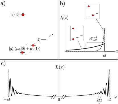
Figure 5: (a) Energy diagram of the initial state: two fermions with blocking atom in a superposition of the motional states $\ket{0}$ and $\ket{1}$. (b) Spatial intensity distribution $I_{t}(x)$ of the emitted photon wavepacket at time $t$ for the limiting cases where the blocking atom is in $\ket{0}$ or $\ket{1}$, respectively. In both cases, the outgoing wavepacket propagates with the speed of light and falls off exponentially with a width $c/((1-\alpha\eta^{2})\Gamma)$ ($c/(\alpha\eta^{2}\Gamma)$) for the initial state $\ket{g1;e0}$ ($\ket{g0;e0}$). (c) The blocking atom is prepared in a superposition of motional states, we choose $\mu_{0}=1-\eta^{2}/2$ and $\mu_{1}=\mathrm{i}\sqrt{1-\mu_{0}^{2}}$. As this is the motional state which the excited atom would reach by sending out a photon along the negative $\hat{\bm{x}}$-axis, emission in this direction is suppressed at the beginning of the atomic decay ($t=0$). Hence, the photon intensity is zero at $x=-ct$ and has a maximum at $x=+ct$. During the decay of the excited atom, the blocking atom oscillates in the trap with a frequency $\nu$, which imprints the spatial period $2\pi c/\nu$ onto the photon wavepacket.

In the previous sections we have discussed the atomic dynamics of the Pauli-blocked decay. In addition, this effect also becomes manifest in the intensity distribution of the emitted photon wavepacket. Compared to the decay in absence of a blocking atom, due to the prolonged lifetime of the excited state, we will see a broader spatial extension of the wavepacket. Furthermore, to some extent a temporal shaping of the emitted photon is possible by preparing the blocking atom initially in a superposition of motional states. For simplicity, we regard the case where the blocking atom is in a superposition of the lowest two motional states (see Fig. 5(a)). This situation captures the essential effect as the contribution of higher motional states in the superposition leads to modifications of order $\eta^{4}$ or less. The photon shaping effect can be most explicitly observed in the regime $\Gamma\ll\nu$, which can be realized in the setup with alkaline earth atoms as discussed above. In this scheme, the appropriate initial state could be prepared after step II, by coherently transferring part of the population of the blocking atom from the motional state $\ket{0}$ to $\ket{1}$.

We study this model system in a Weisskopf-Wigner ansatz, where we have one excitation either in the atomic system or in the radiation field as an one-photon wavepacket. Compared to the previous treatment where we have traced over the radiation field, here the information about the photon is contained. We consider motional excitations of the atoms only in one dimension and additionally, for the excited atom, only include the lowest motional band $\ket{0}$ as shown in Fig. 5(a). Therefore, we do not include the effects of the dipole-dipole interaction and cross-damping. As discussed above, in the limit $\Gamma\ll\nu$, which corresponds to the alkaline-earth case, the effect of these interactions can be suppressed by choosing a sufficiently large detuning in the quenching process.

Within this ansatz, the state can be written as

$$\ket{\psi(t)}=a_{0e}(t)\ket{g0;e0}+a_{1e}(t)\ket{g1;e0}\\ +\smashoperator[]{\sum_{n>m,\bm{k}}^{}}a_{mn,\bm{k}}(t)\ket{gm;gn;1_{\bm{k}}},$$ (11)

where the first two terms correspond to the situation before the decay and the last term corresponds to both atoms in their internal groundstate and an outgoing one-photon wavepacket. The initial condition is $a_{0e}(0)=\mu_{0}$, $a_{1e}(0)=\mu_{1}$, $a_{mn,\bm{k}}(0)=0$ for all $m,n,\bm{k}$ and $\lvert\mu_{0}\rvert^{2}+\lvert\mu_{1}\rvert^{2}=1$. We solve the Schrödinger equation of the Hamiltonian

$$H = \sum_{n}\hbar\omega_{0}c_{en}^{\dagger}c_{en}+\smashoperator[]{\sum_{\sigma\in\left\{e,g\right\},n}^{}}\hbar\nu nc_{\sigma n}^{\dagger}c_{\sigma n}+\sum_{\bm{k}}\hbar\omega_{k}b_{\bm{k}}^{\dagger}b_{\bm{k}}$$

$$-\Bigl{(}\sum_{\bm{k}}\mathcal{E}_{k}\bm{d}_{eg}\cdot\bm{e}_{\bm{k}}b_{\bm{k}}\sum_{n,m}R_{nm}(\hat{\bm{k}}\cdot\hat{\bm{\chi}})c_{en}^{\dagger}c_{gm}+\text{h.c.}\Bigr{)},$$

which consists of internal and center of mass degrees of freedom of the atoms, the free radiation field and the coupling between atoms and field in dipole and rotating wave approximation. Here, in addition to the operators and parameters defined before, $b_{\bm{k}}$ ($b_{\bm{k}}^{\dagger}$) is the annihilation (creation) operator for a photon with frequency $\omega_{k}$ and wave vector (polarization) $\bm{k}$ ($\bm{e}_{\bm{k}}$), $\hat{\bm{\chi}}$ is a unit vector in direction of the 1D harmonic oscillator potential and $\mathcal{E}_{k}=\mathrm{i}\sqrt{\hbar\omega_{k}/(2\varepsilon_{0}L^{3})}$ with quantization volume $L^{3}$. The solution for the coefficients $a_{0e}(t)$, $a_{1e}(t)$ and $a_{mn,\bm{k}}(t)$ is obtained by the standard resolvent method Louisell (1973) and is given in Appendix B.

From the spectral distribution of the photon $a_{mn,\bm{k}}(t)$ we calculate the first order correlation function $I(\bm{r},t)=\braket{\psi(t)}{\bm{E}^{(-)}(\bm{r})\bm{E}^{(+)}(\bm{r})}{\psi(t)}$, which is proportional to the electric field intensity. Here, $\bm{E}^{(+)}(\bm{r})=\sum_{\bm{k}}\mathcal{E}_{k}\bm{e}_{\bm{k}}b_{\bm{k}}\mathrm{e}^{\mathrm{i}\bm{k}\cdot\bm{r}}$ and its hermitian conjugate $\bm{E}^{(-)}(\bm{r})$ is the positive and negative part of the electric field operator, respectively. The probability of detecting a photon between the times $t$ and $t+\mathrm{d}t$ in a volume element $r^{2}\mathrm{d}r\,\mathrm{d}\Omega$ around $\bm{r}$ is proportional to $I(\bm{r},t)r^{2}\mathrm{d}r\,\mathrm{d}\Omega\,\mathrm{d}t$ Glauber (1963).

Let us consider the atomic system placed at the origin of our coordinate system, with $\bm{d}_{eg}$ parallel to the $\hat{\bm{z}}$-axis and $\hat{\bm{\chi}}$ parallel to $\hat{\bm{x}}$. We analyze $I(\bm{r},t)$ in the far zone limit $k_{0}r\gg 1$ and for times $t\gg\Gamma_{\text{eff}}^{-1}$, when the initially excited atom certainly has decayed to the ground state. In the following, we discuss the properties of $I(\bm{r},t)$ along the $\hat{\bm{x}}$-axis where we denote $I(\bm{r},t)r^{2}|_{\bm{r}=(x,0,0)}\equiv I_{t}(x)$. The complete form of $I(\bm{r},t)$ can be found in Appendix B.

For the two limiting cases of the initial state, where all of the population of the blocking atom is either in the motional state $\ket{0}$ or $\ket{1}$ (see Fig. 5(b)), the decay of the excited atom will be maximally blocked or essentially not blocked, respectively. The corresponding decay rates to order $\mathcal{O}(\eta^{2})$ are $\Gamma_{\text{eff}}^{(0)}=\alpha\eta^{2}\Gamma$ and $\Gamma_{\text{eff}}^{(1)}=(1-\alpha\eta^{2})\Gamma$. Consequently, the outgoing exponential photon wave packet, which has a spatial width $c/\Gamma^{(0,1)}_{\text{eff}}$ and propagates with the speed of light $c$, is much broader for the initial state $\ket{g0;e0}$ compared to the case of an initial state $\ket{g1;e0}$.

Let us now consider the case where the blocking atom initially is in a superposition of motional states. As such a state is not an eigenstate of the harmonic trapping potential, the blocking atom oscillates in the trap while the decay of the excited atom takes place. Due to this osciallation, the preferred direction of the emitted photon varies in time. The characteristic frequency for the dynamics in the trap is $\nu$, which is imprinted onto the photon wavepacket as a spatial oscillation with a period $2\pi c/\nu$ (see Fig. 5(c)).

We finally point out that other techniques to induce dynamics for the blocking atom could allow for more sophisticated shaping of the emitted photon. For example, Rabi oscillations could be driven for the blocking atom between $\ket{g0}$ and another, decoupled internal state, or the trapping potential could be modulated during the Pauli-blocked decay.

V Summary and Outlook

In this work we have studied how the Pauli exclusion principle can give rise to a suppression of spontaneous emission from electronically excited states for cold fermionic atoms stored in optical lattices. Here the presence of both a ground state and an excited state atom at the same lattice site can block the dominant decay channel for the excited atom, thereby significantly decreasing the spontaneous emission rate. Complementary to the atomic dynamics we have studied how the decay dynamics in the presence of a blocking atom manifests itself in the characteristics of the emitted photon. We have suggested and analyzed experimental realizations with alkaline earth atoms and also with alkali atoms.

On the one hand, from a conceptual point of view, observing these effects for fermionic atoms in optical lattices would be the first experimental demonstration of Pauli-blocked spontaneous emission. On the other hand, from a more practical perspective, the use of this blocking effect in a controllable way can constitute an additional, valuable tool in the context of reservoir engineering in cold atom systems. Here, the idea of engineering a controlled coupling to an environment for the dissipative preparation of entangled states and many-body quantum phases has been explored both theoretically Diehl et al. (2008); Verstraete et al. (2009); Kraus et al. (2008); Weimer et al. (2010); Cho et al. (2011); Diehl et al. (2011) and in experiments with atomic ensembles Krauter et al. (2010) and trapped ions Barreiro et al. (2011). In particular, for cold fermionic atoms in optical lattices Diehl et al. Diehl et al. (2010) have proposed and analyzed a scenario, where quasi-local single-fermion dissipative processes can be tailored such that they lead to “cooling” into a BCS-type state of $d$-wave symmetry. The corresponding set of fermionic quantum jump operators for the dissipative dynamics are suggested to be implemented via a stroboscopic sequence of coherent and dissipative steps in a system of two-component fermionic alkaline-earth atoms. Here, controlled induced spontaneous decay, which is suppressed (enabled) in the presence (absence) of a second fermionic atom, as studied in the present work, constitutes the dissipative ingredient, which also warrants the required Fermi statistics of the quantum jump operators.

In addition, the possibility to control to some extent the spatial and temporal emission characteristics of the outgoing photon under induced spontaneous decay in the presence of a suitably prepared blocking atom, might constitute an interesting tool in the context of the development of (directed) single-photon sources Grangier et al. (2004).

Appendix A Recoil matrix elements and initial Pauli-blocked decay rate

In Eqs. (6) and (8), the recoil matrix elements $R_{\bm{m}\bm{n}}(\hat{\bm{k}})\equiv\prod_{j=1,2,3}R_{m_{j}n_{j}}(\hat{k}_{j})$ are given by

$$R_{m_{j}n_{j}}(\hat{k}_{j})=\mathrm{e}^{-\hat{k}_{j}^{2}\eta_{j}^{2}/2}\sqrt{\frac{\min(m_{j},n_{j})!}{\max(m_{j},n_{j})!}}(-\mathrm{i}\hat{k}_{j}\eta_{j})^{\lvert m_{j}-n_{j}\rvert}\\ \times L_{\min(m_{j},n_{j})}^{\lvert m_{j}-n_{j}\rvert}(\hat{k}_{j}^{2}\eta_{j}^{2}),$$

where

$$L_{b}^{c}(x) =\sum_{j=0}^{b}(-1)^{j}\binom{b+c}{b-j}\frac{x^{j}}{j!}$$

is the generalized Laguerre polynomial. For a tight trapping in the Lamb-Dicke limit, the recoil matrix elements can be expanded in the small parameter $\eta_{j}\ll 1$. To order $\eta_{j}^{2}$, the result is

$$R_{m_{j}n_{j}}(\hat{k}_{j}) \approx\begin{cases}1-(m+\frac{1}{2})\hat{k}_{j}^{2}\eta_{j}^{2}\ &\text{for $m_{j}=n_{j}$}\\ -\mathrm{i}\hat{k}_{j}\eta_{j}\sqrt{m}&\text{for $\lvert m_{j}-n_{j}\rvert=1$}\\ -\frac{1}{2}\hat{k}_{j}^{2}\eta_{j}^{2}\sqrt{m(m-1)}&\text{for $\lvert m_{j}-n_{j}\rvert=2$,}\end{cases}$$

where we have defined $m=\max(m_{j},n_{j})$. The dominant matrix elements are those with $m_{j}=n_{j}$, whereas matrix elements with $\lvert m_{j}-n_{j}\rvert=1$ and $\lvert m_{j}-n_{j}\rvert=2$ are of order $\eta_{j}$ and $\eta_{j}^{2}$, respectively.

The master equation coefficients $\tilde{R}_{\bm{n}^{\prime}\bm{m}^{\prime}\bm{m}\bm{n}}$ defined in Eq. (7) are real, because of parities they are zero if any of the three components of $\bm{n}^{\prime}+\bm{m}^{\prime}+\bm{m}+\bm{n}$ is odd, and they are invariant under exchange $(\bm{n}^{\prime}\bm{m}^{\prime})\leftrightarrow(\bm{m}\bm{n})$ and under exchange $n^{\prime}_{j}\leftrightarrow m^{\prime}_{j}$ or $m_{j}\leftrightarrow n_{j}$ for any $j=1,2,3$. In Lamb-Dicke expansion to order $\eta_{j}^{2}$, the only contributing coefficients are those with (i) $\bm{m}=\bm{n}$ and $\bm{m}^{\prime}=\bm{n}^{\prime}$, (ii) $\lvert m_{j}-n_{j}\rvert=\lvert m^{\prime}_{j}-n^{\prime}_{j}\rvert=\delta_{i,j}$ for an $i\in\left\{1,2,3\right\}$, (iii) $\bm{m}=\bm{n}$ and $\lvert m^{\prime}_{j}-n^{\prime}_{j}\rvert=2\delta_{i,j}$ for an $i\in\left\{1,2,3\right\}$ (or vice versa). In these cases, we find

$$R_{\bm{n}^{\prime}\bm{m}^{\prime}\bm{m}\bm{n}} \approx\begin{cases}1-\sum_{j}(m^{\prime}_{j}+m_{j}+1)\alpha_{j}\eta_{j}^{2}&\ \text{(i)}\\ \alpha_{i}\eta_{i}^{2}\sqrt{m^{\prime}m}&\ \text{(ii)}\\ -\frac{1}{2}\alpha_{i}\eta_{i}^{2}\sqrt{m^{\prime}(m^{\prime}-1)}&\ \text{(iii)},\end{cases}$$ (12)

where $m^{\prime}=\max(m_{i}^{\prime},n_{i}^{\prime})$, $m=\max(m_{i},n_{i})$. The numerical coefficients $\alpha_{j}=\frac{1}{5}(2-\lvert\hat{d}_{eg,j}\rvert^{2})$ with $\frac{1}{5}\leq\alpha_{j}\leq\frac{2}{5}$ and $\sum_{j}\alpha_{j}=1$ depend on the projection of the transitions dipole matrix element onto the $j$-axis.

The total initial decay rate $\Gamma_{\text{eff}}$ defined in Eq. (9) can be written as

$$\Gamma_{\text{eff}} =\Gamma\left(1-R_{\bm{0}\bm{0}\bm{0}\bm{0}}\right),$$

which in the general case can be evaluated numerically. For the case of tight trapping in the Lamb-Dicke limit, by using Eq. (12), it is given by $\Gamma_{\text{eff}}=\sum_{j=1,2,3}\alpha_{j}\eta_{j}^{2}\Gamma+\mathcal{O}(\eta_{j}^{4})$.

Appendix B Weisskopf-Wigner approach

For times $t\gg\Gamma_{\text{eff}}^{-1}$, the solution of the Weisskopf-Wigner ansatz Eq. (11) in terms of the coefficients $a_{01,\bm{k}}(t)$, $a_{0n,\bm{k}}(t)$, $a_{1n,\bm{k}}(t)$ with $n>1$ is Louisell (1973)

$$a_{01,\bm{k}}(t) =\mathcal{E}_{k}^{\ast}\bm{d}_{eg}\cdot\bm{e}_{\bm{k}}\mathrm{e}^{-\mathrm{i}(\omega_{k}+\nu)t}\left(\frac{\mu_{0}R_{01}^{\ast}(\hat{\bm{k}}\cdot\hat{\bm{\chi}})}{\hbar\left((\omega_{k}+\nu-\omega_{0})+\mathrm{i}\Gamma^{(0)}_{\text{eff}}/2\right)}-\frac{\mu_{1}R_{00}^{\ast}(\hat{\bm{k}}\cdot\hat{\bm{\chi}})}{\hbar\left((\omega_{k}-\omega_{0})+\mathrm{i}\Gamma^{(1)}_{\text{eff}}/2\right)}\right)$$

$$a_{0n,\bm{k}}(t) =\mathcal{E}_{k}^{\ast}\bm{d}_{eg}\cdot\bm{e}_{\bm{k}}\mathrm{e}^{-\mathrm{i}(\omega_{k}+n\nu)t}\frac{\mu_{0}R_{0n}^{\ast}(\hat{\bm{k}}\cdot\hat{\bm{\chi}})}{\hbar\left((\omega_{k}+n\nu-\omega_{0})+\mathrm{i}\Gamma^{(0)}_{\text{eff}}/2\right)}$$

$$a_{1n,\bm{k}}(t) =\mathcal{E}_{k}^{\ast}\bm{d}_{eg}\cdot\bm{e}_{\bm{k}}\mathrm{e}^{-\mathrm{i}(\omega_{k}+(n+1)\nu)t}\frac{\mu_{1}R_{0n}^{\ast}(\hat{\bm{k}}\cdot\hat{\bm{\chi}})}{\hbar\left((\omega_{k}+(n+1)\nu-\omega_{0})+\mathrm{i}\Gamma^{(1)}_{\text{eff}}/2\right)},$$

where $\Gamma^{(0)}_{\text{eff}}=\alpha\eta^{2}\Gamma+\mathcal{O}(\eta^{4})$ ($\Gamma^{(1)}_{\text{eff}}=(1-\alpha\eta^{2})\Gamma+\mathcal{O}(\eta^{4})$) is the effective decay rate for the initial state $\ket{g0;e0}$ ($\ket{g1;e0}$). All other coefficients $a_{mn,\bm{k}}(t)$ with $n>m$ are zero within this model. The first order correlation function $I(\bm{r},t)$ can be written as Scully and Zubairy (1997)

$$I(\bm{r},t) = \lvert\bm{\Psi}_{1}(\bm{r},t)\rvert^{2}+\sum_{n>1}\left[\lvert\bm{\Psi}_{n}^{(0)}(\bm{r},t)\rvert^{2}+\lvert\bm{\Psi}_{n}^{(1)}(\bm{r},t)\rvert^{2}\right]$$

$$\lvert\bm{\Psi}_{1}(\bm{r},t)\rvert^{2} = \frac{d_{eg}^{2}\omega_{0}^{4}\sin^{2}\theta}{(4\pi\varepsilon_{0})^{2}c^{2}r^{2}}\Theta(t-r/c)$$

$$\times\Bigl{\{}\lvert\mu_{0}\rvert^{2}\lvert R_{01}(u)\rvert^{2}\exp\left(-\Gamma^{(0)}_{\text{eff}}(t-r/c)\right)+\lvert\mu_{1}\rvert^{2}\lvert R_{00}(u)\rvert^{2}\exp\left(-\Gamma^{(1)}_{\text{eff}}(t-r/c)\right)\Bigr{.}$$

$$\Bigl{.}-2\real\left(\mu_{0}R_{01}^{\ast}(u)\mu_{1}^{\ast}R_{00}(u)\exp\left(\mathrm{i}\nu(t-r/c)\right)\exp\left(-(\Gamma^{(0)}_{\text{eff}}+\Gamma^{(1)}_{\text{eff}})(t-r/c)/2\right)\right)\Bigr{\}}$$

$$\lvert\bm{\Psi}_{n}^{(0,1)}(\bm{r},t)\rvert^{2} = \frac{d_{eg}^{2}\omega_{0}^{2}\sin^{2}\theta\lvert\mu_{0,1}\rvert^{2}\lvert R_{0n}(u)\rvert^{2}}{(4\pi\varepsilon_{0})^{2}c^{2}r^{2}}\Theta(t-r/c)\exp\left(-\Gamma^{(0,1)}_{\text{eff}}(t-r/c)\right).$$

where $\theta$ is the angle between $\bm{r}$ and $\bm{d}_{eg}$, $u=\hat{\bm{r}}\cdot\hat{\bm{\chi}}$ and $\Theta$ is the Heaviside step function.

References

- Kleppner (1981) D. Kleppner, Phys. Rev. Lett., 47, 233 (1981).
- Noda et al. (2007) S. Noda, M. Fujita, and T. Asano, Nature photonics, 1, 449 (2007).
- Jhe et al. (1987) W. Jhe, A. Anderson, E. A. Hinds, D. Meschede, L. Moi, and S. Haroche, Phys. Rev. Lett., 58, 666 (1987).
- Busch et al. (1998) T. Busch, J. R. Anglin, J. I. Cirac, and P. Zoller, Europhys. Lett., 44, 1 (1998).
- Shuve and Thywissen (2010) B. Shuve and J. Thywissen, J. Phys. B-At. Mol. Opt., 43, 15301 (2010).
- Ye et al. (2008) J. Ye, H. J. Kimble, and H. Katori, Science, 320, 1734 (2008).
- Derevianko and Katori (2011) A. Derevianko and H. Katori, Rev. Mod. Phys., 83, 331 (2011).
- Daley et al. (2008) A. J. Daley, M. M. Boyd, J. Ye, and P. Zoller, Phys. Rev. Lett., 101, 170504 (2008).
- Fukuhara et al. (2009) T. Fukuhara, S. Sugawa, M. Sugimoto, S. Taie, and Y. Takahashi, Phys. Rev. A, 79, 041604 (2009).
- Cazalilla et al. (2009) M. Cazalilla, A. Ho, and M. Ueda, New J. Phys., 11, 103033 (2009).
- Gorshkov et al. (2010) A. Gorshkov, M. Hermele, V. Gurarie, C. Xu, P. Julienne, J. Ye, P. Zoller, E. Demler, M. Lukin, and A. Rey, Nat. Phys., 6, 289 (2010).
- Swallows et al. (2011) M. Swallows, M. Bishof, Y. Lin, S. Blatt, M. Martin, A. Rey, and J. Ye, Science, 331, 1043 (2011).
- Daley (2011) A. Daley, Arxiv preprint arXiv:1106.5712 (2011).
- Bloch et al. (2008) I. Bloch, J. Dalibard, and W. Zwerger, Rev. Mod. Phys., 80, 885 (2008).
- Lewenstein et al. (2007) M. Lewenstein, A. Sanpera, V. Ahufinger, and B. Damski, Adv. Phys., 56, 243 (2007).
- Jaksch and Zoller (2005) D. Jaksch and P. Zoller, Ann. Phys., 315, 52 (2005).
- Kraus et al. (2008) B. Kraus, H. P. Büchler, S. Diehl, A. Kantian, A. Micheli, and P. Zoller, Phys. Rev. A, 78, 042307 (2008).
- Diehl et al. (2008) S. Diehl, A. Micheli, A. Kantian, B. Kraus, H. P. Büchler, and P. Zoller, Nat. Phys., 4, 878 (2008).
- Verstraete et al. (2009) F. Verstraete, M. M. Wolf, and J. I. Cirac, Nat. Phys., 5, 633 (2009).
- Weimer et al. (2010) H. Weimer, M. Müller, I. Lesanovsky, P. Zoller, and H. P. Büchler, Nat. Phys., 6, 382 (2010).
- Cho et al. (2011) J. Cho, S. Bose, and M. S. Kim, Phys. Rev. Lett., 106, 020504 (2011).
- Diehl et al. (2011) S. Diehl, E. Rico, M. Baranov, and P. Zoller, Arxiv preprint arXiv:1105.5947 (2011).
- Krauter et al. (2010) H. Krauter, C. Muschik, K. Jensen, W. Wasilewski, J. Petersen, J. Cirac, and E. Polzik, Arxiv preprint arXiv:1006.4344 (2010).
- Barreiro et al. (2011) J. Barreiro, M. Müller, P. Schindler, D. Nigg, T. Monz, M. Chwalla, M. Hennrich, C. F. Roos, P. Zoller, and R. Blatt, Nature, 470, 486 (2011).
- Diehl et al. (2010) S. Diehl, W. Yi, A. J. Daley, and P. Zoller, Phys. Rev. Lett., 105, 227001 (2010).
- Louisell (1973) W. Louisell, Quantum statistical properties of radiation (John Wiley and Sons, Inc., New York, 1973).
- Katori et al. (2003) H. Katori, M. Takamoto, V. G. Pal’chikov, and V. D. Ovsiannikov, Phys. Rev. Lett., 91, 173005 (2003).
- Poyatos et al. (1996) J. F. Poyatos, J. I. Cirac, R. Blatt, and P. Zoller, Phys. Rev. A, 54, 1532 (1996).
- Reichenbach and Deutsch (2007) I. Reichenbach and I. H. Deutsch, Phys. Rev. Lett., 99, 123001 (2007).
- Lehmberg (1970) R. H. Lehmberg, Phys. Rev. A, 2, 889 (1970).
- Kazantsev et al. (1990) A. P. Kazantsev, G. I. Surdutovich, and V. P. Yakovlev, Mechanical action of light on atoms (World Scientific, 1990).
- Pichler et al. (2010) H. Pichler, A. J. Daley, and P. Zoller, Phys. Rev. A, 82, 063605 (2010).
- Boyd et al. (2007) M. M. Boyd, T. Zelevinsky, A. D. Ludlow, S. Blatt, T. Zanon-Willette, S. M. Foreman, and J. Ye, Phys. Rev. A, 76, 22510 (2007).
- Porsev et al. (2004) S. G. Porsev, A. Derevianko, and E. N. Fortson, Phys. Rev. A, 69, 21403 (2004).
- Kohno et al. (2009) T. Kohno, M. Yasuda, K. Hosaka, H. Inaba, Y. Nakajima, and F.-L. Hong, Appl. Phys. Expr., 2, 072501 (2009).
- Barber et al. (2006) Z. W. Barber, C. W. Hoyt, C. W. Oates, L. Hollberg, A. V. Taichenachev, and V. I. Yudin, Phys. Rev. Lett., 96, 083002 (2006).
- Viverit et al. (2004) L. Viverit, C. Menotti, T. Calarco, and A. Smerzi, Phys. Rev. Lett., 93, 110401 (2004).
- Köhl et al. (2005) M. Köhl, H. Moritz, T. Stöferle, K. Günter, and T. Esslinger, Phys. Rev. Lett., 94, 80403 (2005).
- Santra et al. (2005) R. Santra, E. Arimondo, T. Ido, C. H. Greene, and J. Ye, Phys. Rev. Lett., 94, 173002 (2005).
- Baumann and Wandel (1968) M. Baumann and G. Wandel, Phys. Lett. A, 28, 200 (1968).
- Olschewski and Otten (1967) L. Olschewski and E. W. Otten, Z. Phys. A., 200, 224 (1967).
- Berends and Maleki (1992) R. W. Berends and L. Maleki, J. Opt. Soc. Am. B, 9, 332 (1992).
- Glauber (1963) R. J. Glauber, Phys. Rev., 130, 2529 (1963).
- Grangier et al. (2004) P. Grangier, B. Sanders, and J. Vuckovic, New J. Phys., 6 (2004).
- Scully and Zubairy (1997) M. Scully and M. Zubairy, Quantum Optics (Cambridge University press, 1997).