Molecular-spin dynamics study of electromagnons in multiferroic RMn₂O₅

Abstract

We investigate the electromagnon in magnetoferroelectrics RMn₂O₅ using combined molecular-spin dynamics simulations. We identify the origin of the electromagnon modes observed in the optical spectra and reproduce the most salient features of the electromagnon in these compounds. We find that the electromagnon frequencies are very sensitive to the magnetic wave vector along the $a$ direction. We further investigate the electromagnon in magnetic field. Although the modes frequencies change significant under magnetic field, the static dielectric constant electromagnon does not change much in the magnetic field.

Magnetoferrelectrics with strong magnetoelectric (ME) couplings have attracted intensive attention for their novel physics Hur et al. (2004a); Kimura et al. (2003); Goto et al. (2004); Hur et al. (2004b) and potential applications in tunable multifunctional devicesCheong and Mostovoy (2007); Fiebig (2005). One of the most attractive features of the magnetoferroelectrics is that the spin waves and infrared phonons could couple via ME interactions leading to a new type of elementary excitation, electromagnon Smolenskii and Chupis (1982). Electromagnon has mixed characters of both magnons and infrared phonons. It therefore opens a way to control the magnetic excitations via electric fields Mochizuki and Nagaosa (2010), which may have important applications for information processes. However, despite electromagnon has been proposed theoretically almost four decades ago, it has been observed experimentally only very recently Pimenov et al. (2006). Till today, our knowledge about electromagnon is still very limited.

In the past few years, electromagnon has been observed in various magnetoferroelectrics, mostly in the family of RMnO₃Pimenov et al. (2006); Aguilar et al. (2007) and RMn₂O₅ Sushkov et al. (2007) (R =Tb, Dy, Gd, Eu, Y) compounds. So far, most theoretical works on electromagnon were concentrated on the RMnO₃ familyKatsura et al. (2007); Aguilar et al. (2009); Mochizuki et al. (2010), because they have relatively simpler magnetic structures, containing only Mn³⁺ ions. The study of electromagnon in RMn₂O₅ is still very few both experimentallySushkov et al. (2007); kim and theoretically Sushkov et al. (2008), due to the complexity of the magnetic structures in these compounds. A simulation of the electromagnon in RMn₂O₅ at atomistic level is still lack. It has been shown experimentally that the dielectric step at the commensurate (CM) to incommensurate (ICM) magnetic phase transition in RMn₂O₅ is caused by the electromagnon Sushkov et al. (2007). However, it is still unclear how the electromagnon is related to the magnetodielectric effect, which also happens at the same temperature and is one of the most prominent effects in these materials Hur et al. (2004a).

In this work, we carry out combined molecular-spin dynamics(MSD) simulations to study electromagnons in RMn₂O₅. We reproduce the most salient features of the electromagnon in these compounds and find that the electromagnons frequencies are very sensitive to the magnetic wave vector along the $a$ direction. We further investigate the behavior of electromagnon under magnetic fields, and find that although the mode frequency change significant under magnetic field, the static dielectric constant electromagnon does not change much in the magnetic field in our model.

To study the electromagnon in RMn₂O₅, we use the effective Hamiltonian derived in Ref. Wang et al. (2008); Cao et al. (2009),

$$H=\sum_{k}{1\over 2}m\omega^{2}u_{k}^{2}-\sum_{ij\in{J_{\alpha}}}J_{\alpha}(0){\bf S}_{i}\cdot{\bf S}_{j}-\sum_{ij\in{J_{3}}}\sum_{k}J_{3}^{\prime}\,u_{k}{\bf S}_{i}\cdot{\bf S}_{j}+\sum_{kl}\xi_{kl}u_{k}\cdot u_{l}-\sum_{i}(K_{i}\cdot{\bf S}_{i})^{2}+\sum_{i}D_{i}(S_{i}^{c})^{2}-g\sum_{i}{\bf H}\cdot{\bf S}_{i}.$$ (1)

where $J_{3}$ is the Mn⁴⁺- Mn³⁺ superexchange interaction through pyramidal base corners, and $J_{4}$ the superexchange interaction through the pyramidal apex Chapon et al. (2004). Mn³⁺ couples to Mn⁴⁺ either antiferromagnetically via $J_{4}$ along $a$ axis or with alternating sign via $J_{3}$ along $b$ axis, whereas Mn³⁺ ions in two connected pyramids couple each other antiferromagnetically through $J_{5}$. $J_{1}$, $J_{2}$ couple Mn⁴⁺ ions along the $c$ axis. $u$ is an artificial optical phonon to describe the electric polarization Wang et al. (2008); Cao et al. (2009). In RMn₂O₅, the infrared modes that couple to the electromagnon are the same modes that causes the marcoscopic polarization. This is very different from those in RMnO₃ compounds. One can find more details of the model in Ref. Cao et al. (2009). The major difference between the current model and previous onesWang et al. (2008); Cao et al. (2009) is that we include here the single ion easy axis anisotropy $K_{3}$ for Mn³⁺ ions and the easy plane anisotropies $D_{i}$ for Mn³⁺ and Mn⁴⁺ ions to describe the magnetic anisotropy in these compounds. H is the applied magnetic field and $g$ is gyromagnetic ratio.

We use the model parameters obtained in Ref. Cao et al. (2009) until otherwise noticed. Since accurate magnetic anisotropy energies are still very hard to obtain from the current first-principles methods, especially for complex materials like RMn₂O₅, we use empirical anisotropy parameters to fit the experimental magnetization and optical spectra.

We carry out MSD simulations of the Hamiltonian by solving the coupled equations of motion of spin and phonon using forth-order Runge-Kutta method,

$$\hbar\dot{{\bf S}_{i}} = -{\bf S}_{i}\times{\bf H}^{eff}_{i}$$ (2)

$$\ddot{u}_{k} = {\bf F}_{k}/m$$ (3)

where ${\bf H}^{eff}_{i}=-\partial H/\partial{\bf S}_{i}$ is the effective magnetic field acting on the $i$th Mn spin ${\bf S}_{i}$ and ${\bf F}_{k}=-\partial H/\partial u_{k}$ is the force acting on the $k$th local phonon mode. Since Mn³⁺ and Mn⁴⁺ have 4 and 3 unpaired local $d$ electron respectively, we set the norm of Mn${}_{3}^{+}$ spin vector $|{\bf S}_{3}|=\sqrt{2(2+1)}$ and the norm of Mn${}_{4}^{+}$ spin vector $|{\bf S}_{4}|=\sqrt{1.5(1.5+1)}$. Unlike previous methods Mochizuki et al. (2010), our method takes the phonon degree of freedom into consideration explicitly.

We start the MSD simulation from a pool of equilibrium configurations sampled from MC simulation at a given temperature $T$. The system is further relaxed for sufficient time in the MSD simulations. Simulations with different initial configurations are averaged to realize a canonical assemble at fixed $T$ Landau and Krech (1999). The optical spectrum Im$\chi(\omega)$ is calculated from the Fourier-Laplace transform of correlation function $\Phi(t)$ of dipole moment P(t) with $\Phi(t)=\langle P(t)P(0)\rangle-\langle P(t)\rangle\langle P(0)\rangle$, i.e.,

$$Im\chi(\omega)=\frac{\omega Re{\mathcal{L}[\Phi]}}{K_{B}T}$$ (4)

where $P(t)=\sum_{k}u_{k}(t)$ and $\langle\cdots\rangle$ represents the ensemble average. The static susceptibility $\chi(0)$ can be calculated as,

$$\chi(0)=\frac{\Phi(0)}{K_{B}T}\,,$$ (5)

where $K_{B}$ is the Boltzman constant. To extract the detailed parameters of the spectral weight, we fit $\chi(\omega)$ to a lorentz model,

$$\chi(\omega)=\sum_{j}{\frac{S_{j}}{\omega_{j}^{2}-\omega^{2}-2i\gamma_{j}\omega}}$$ (6)

where $j$ enumerates the vibrations, $\omega_{j}$ is the resonance frequency, and $\gamma_{j}$ is the damping rate. To avoid numerical errors, we fit directly the correlation function $\Phi(t)$, which can be analytically Fourier transformed to lorentz model in Eq. 6. The static electric susceptibility is the sum of all oscillators strengths, $\chi(0)=\sum_{j}\frac{S_{j}}{\omega^{2}_{j}}$. According to the sum rule, the total spectral weight $S=\sum_{j}S_{j}$ should be conserved.

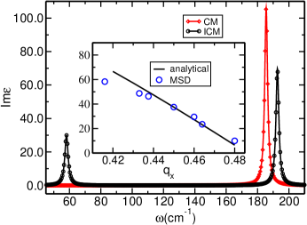
Figure 1: (Color online). The imagery part of the dielectric response Im$\chi(\omega)$ calculated using the $12\times 12\times 12$ lattice in the CM magnetic phase (red) and the ICM magnetic phase (black). Inset: The electromagnon frequency as function of the magnetic wave vector along $a$ direction $q_{x}$. Circles represents the electromagnon frequency calculated by MSD, whereas the black line is calculated from $J_{5}\sin(2\pi q_{x})-14.63$ cm^-1.

We first compare the MSD results to previous MC simulations Cao et al. (2009), by carrying out the MSD simulation in a 12$\times$12$\times$12 lattice at various temperatures, without including the magnetic anisotropy. The imaginary part of the dielectric response Im$\chi(\omega)$ of the CM phase at 20K and ICM phase at 3K is shown in Fig. 1. We can see that, in the CM phase, there is only one peak centered at about 185 cm^-1, corresponding to the bare phonon frequency in our model. While at ICM phase, there are two peaks: one is the phonon peak at about 193 cm^-1 which is hardened compared to the bare phonon frequency due to strong spin-phonon coupling foo (a), and the new peak appear at about 58 cm^-1 is the electromagnon.

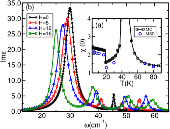
Figure 2: (Color online) (a) The static dielectric susceptibility $\chi$(0) as functions of temperature calculated using MC and MSD. (a) The imaginary part of the dielectric response Im $\varepsilon(\omega)$ of RMn₂O₅ under different magnetic fields.

The calculated $\chi(0)$ is shown in Fig. 2(a) at different temperatures compared with those obtained from MC simulations Cao et al. (2009). We see that $\chi(0)$ calculated from both MC and MSD shows a step at the CM to ICM transition. The difference between $\chi(0)$ calculated with MC an MSD comes from the long-time relaxation effects that are not included in the MSD simulation. The results are in remarkable agreement with the experimental results of Ref. Sushkov et al., 2007. Although electromagnons have been successfully reproduced using our model, the frequency of the electromagnon mode is much higher than the experimental values for TbMn₂O₅ and YMn₂O₅Sushkov et al. (2007). Further examinations show that the electromagnon frequencies are very sensitive to the $x$ component of wave vector $q_{x}$. In the ICM phase, the spins connected by the strongest interaction $J_{4}$ are almost parallel to each otherCao et al. (2009), and the spiral along $a$ direction comes from the spins connected by $J_{5}$, with an angle of 2$\pi q_{x}$. Since the electromagnon excitation is at Brillouin zone center, $J_{4}$ makes no contribution to the electromagnon as can be easily seen from Eq. 2, whereas the second largest exchange interaction $J_{5}$ dominates the interaction. We therefore expect the energy of the electromagnon $\sim J_{5}\sin(2\pi q_{x})$. To confirm this result, we simulate the electromagnon on a larger 50$\times$6$\times$6 lattice and adjust the parameter slightly to obtain different $q_{x}$ of the ICM state. The calculated lowest electromagnon mode frequencies at different $q_{x}$ are shown in the insert of Fig. 1. As we see that the electromagnon frequencies decrease significantly as $q_{x}$ approaching $\pi/2$, showing nice agreement with $J_{5}\sin(2\pi q_{x})-14.63$cm^-1. At $q_{x}$=0.48, the electromagnon frequency decreases to about 10 cm^-1, which is in good agreement with experiments Sushkov et al. (2007). Most of the RMn₂O₅ (R=Tb, Ho, …) compounds have $q_{x}\sim$ 0.48, therefore the electromagnon frequencies in these materials should be very similar. However, we expect that the electromagnons in TmMn₂O₅Kobayashi et al. (2005), with $q_{x}$ $\sim$ 0.467, should have much higher frequencies. Experimental confirm of this prediction is called for.

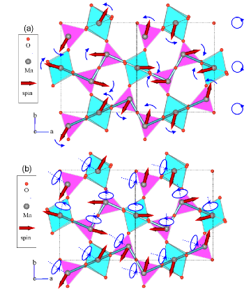
Figure 3: (Color online) The cartoons of two identified electromagnon modes. The blue arrows denote rotation direction. (a) The “phason” mode, where spins in the same chain rotate in the same direction as a unit. (b) The highest frequency electromagnon mode appear under magnetic field H $\parallel a$. The blue arrows denote rotation directions.

We now look into more details of the electromagonons in the ICM phase. To compare better with the experiments, we slightly modify our model parameters to $J_{3}$=1.5 meV and $J_{3}^{\prime}$=0.3 meV to get $q_{x}$=0.46 in the 50$\times$6$\times$6 lattice foo (b). Though the frequencies are a little higher than the experimental data, it does not change the basic physics of our model. To see how the magnetic anisotropy affect the electromagnon, we also include the ionic anisotropy energies in the simulation. We take $D_{3}=0.09$ meV, $D_{4}=0.06$ meV and three typical in-plane easy axis anisotropy energies $K_{3}$=(0.19, $\pm$ 0.21, 0), (0.278, $\pm$0.082, 0), (0.08 $\pm$0.28, 0), corresponding to the case of Dy, Tb and Ho respectively. We first show the results using $K_{3}$=(0.19, $\pm$ 0.21, 0).

The imaginary part of the dielectric response Im $\varepsilon(\omega)$ at 3K are presented in Fig. 2. After adding the magnetic anisotropy, the original electromagnon peak splits into three modes , centered at 30 cm^-1, 46 cm^-1, 51 cm^-1, respectively, consistent with recent experiments Sushkov et al. (2007); kim . To extract the electromagnon modes, a short electrical pulse $E\parallel b$ at $t=0$ is applied at the equilibrium ground states. The time evolution of each spin is calculated and stored. The electromagnon normal modes are reconstructed from the Fourier transform of each spin motion. From the calculated mode profiles, we confirm that the strongest and lowest frequency peak is the optical counterpart of “phason” with wave vector Q=0. The pattern of the mode is shown in Fig.3(a), which corresponds to the spin rotation in the spiral plane kim . In this mode, the spins of neighboring AFM chains rotate in opposite directions, and couple to phonon modes through the term $J_{3}^{\prime}\,u{\bf S}_{i}\cdot{\bf S}_{j}\,$ forming an electromagnon. We do not obtain a clear profile of the other two modes, because they are relatively weak and mixed with other modes.

Magnetodielectric effect is one of the most prominent effects in RMn₂O₅. To clarify the relation between the electromagnon and magnetodielectric effect, it is important to study the electromagnon in the magnetic field. Figure 2 depicts the imaginary part of dielectric response for $H$=8, 12, 16 $T$ $\parallel a$ direction. Interestingly, there is a new electromagnon peak emerges in the magnetic field above the three electromagnon modes of the zero magnetic field. The new mode can be characterized as spins rotating around an axis perpendicular to itself in the $ab$ plane, as shown in Fig.3(b). We find that the pattern of the lowest frequency mode does not change. and the magnitude of the intermediate two modes are getting stronger in magnetic field. The frequencies of the two lowest electromagnon peaks shift down with the increase of magnetic field and the frequency of the lowest mode shifts down by about 17% under $H$=16$T$ compared to that of zero field. In contrast, the two high frequency modes shift toward even higher frequency with increasing of the magnetic field. To identify the driving force for electromagnon frequency shifts, we compare the magnetic structure with and without magnetic field and find that they are almost the same. Therefore, the frequency shifts mainly come from the dynamic contribution of Zeeman term $-g\sum_{i}{\bf H}\cdot{\bf S}_{i}$.

In spite of the large frequency change in magnetic field, the total static susceptibility calculated from MSD remain almost unchanged compared with that at $H$=0. The total spectral weight also conserves well as the magnetic field increases, within numerical errors. The most contribution to $\chi(0)$ always comes from the lowest electromagnon. At zero magnetic field, the intermediate two electromagnon modes have negligible contribution to the overall $\chi(0)$. Under magnetic field, the lowest electromagnon transfers spectral weight to higher ones, e.g. $50\%$ at H=16 $T$. Therefore although the frequency decreases significantly, $\chi(0)$ calculated from MSD almost keep constant.

We also study the electromagnon in magnetic fields with H$\parallel b$ and H $\parallel c$. The results for H $\parallel b$ are similar to those for H $\parallel a$, while H $\parallel c$ has weak influence on electromagnon both in frequency and spectral weight. Our simulations suggest that the magnetodielectric effects in TbMn₂O₅ are not caused by the electromagnon, but it does not rule out such possibility for DyMn₂O₅, which has unique magnetic structure in the ICM phase, with $q_{x}$=0.5. We also do the simulations using two other $K_{3}$ parameters, and obtained very similar results.

The behaviors of electromagnons in RMn₂O₅ are very different from those in DyMnO₃ where the electromagnon shows a soft-mode behavior in magnetic field $H\parallel a$ and lead to the increase of dielectric constantShuvaev et al. (2010) in the field. This is probably because the magnetic structures of DyMnO₃ are much more sensitive to the applied magnetic field.

To summarize, we investigated the electromagnon in magnetoferroelectrics RMn₂O₅ using combined molecular-spin dynamics simulations. We have identified the origin of the electromagnons in these compounds, and reproduced the most salient features of the electromagnon in these compounds. We find that the electromagnon frequencies are very sensitive to the magnetic wave vector along the $a$ direction. We further investigate the electromagnon in magnetic field. Although the mode frequency change significant under magnetic field, the static dielectric constant does not change much in the magnetic field in our model.

LH acknowledges the support from the Chinese National Fundamental Research Program 2011CB921200 and National Natural Science Funds for Distinguished Young Scholars.

References

- Hur et al. (2004a) N. Hur, S. Park, P. A. Sharma, S. Guha, and S.-W. Cheong, Phys. Rev. Lett. 93, 107207 (2004a).
- Kimura et al. (2003) T. Kimura, T. Goto, H. Shintani, K. Ishizaka, T. Arima, and Y. Tokura1, Nature(Landon) 426, 55 (2003).
- Goto et al. (2004) T. Goto, T. Kimura, G. Lawes, A. P. Ramirez, and Y. Tokura, Phys. Rev. Lett. 92, 257201 (2004).
- Hur et al. (2004b) N. Hur, S. Park, P. A. Sharma, J. S. Ahn, S. Guha, and S.-W. Cheong, Nature (London) 429, 392 (2004b).
- Cheong and Mostovoy (2007) S.-W. Cheong and M. Mostovoy, Nature Materials 6, 13 (2007).
- Fiebig (2005) M. Fiebig, J. Phys. D: Appl. Phys. 286, R123 (2005).
- Smolenskii and Chupis (1982) G. Smolenskii and I. Chupis, Sov. Phys. Usp. 25, 475 (1982).
- Mochizuki and Nagaosa (2010) M. Mochizuki and N. Nagaosa, Phys. Rev. Lett. 105, 147202 (2010).
- Pimenov et al. (2006) A. Pimenov, A. A. Mukhin, V. Ivanov, V. Travkin, A. Balbashov, and A. Loidl, Nature Phys 2, 97 (2006).
- Aguilar et al. (2007) R. V. Aguilar, A. B. Sushkov, C. L. Zhang, Y. J. Choi, S.-W. Cheong, and H. D. Drew, Phys. Rev. B 76, 060404(R) (2007).
- Sushkov et al. (2007) A. B. Sushkov, R. V. Aguilar, S. Park, S.-W. Cheong, , and H. D. Drew, Phys. Rev. Lett. 98, 027202 (2007).
- Katsura et al. (2007) H. Katsura, A. V. Balatsky, and N. Nagaosa, Phys. Rev. Lett. 98, 027203 (2007).
- Aguilar et al. (2009) R. V. Aguilar, M. Mostovoy, A. B. Sushkov, C. L. Zhang, Y. J. Choi, S.-W. Cheong, and H. D. Drew, Phys. Rev. Lett. 102, 047203 (2009).
- Mochizuki et al. (2010) M. Mochizuki, N. Furukawa, and N. Nagaosa, Phys. Rev. Lett. 104, 177206 (2010).
- (15) J.-H. Kim et al, arXiv:1008.5354v1.
- Sushkov et al. (2008) A. B. Sushkov, M. Mostovoy, R. V. Aguilar, S-WCheong, and H. D. Drew, J. Phys.: Condens. Matter 20, 434210 (2008).
- Wang et al. (2008) C. Wang, G.-C. Guo, and L. He, Phys. Rev. B 77, 134113 (2008).
- Cao et al. (2009) K. Cao, G.-C. Guo, D. Vanderbilt, and L. He, Phys. Rev. Lett. 103, 257201 (2009).
- Chapon et al. (2004) L. C. Chapon, G. R. Blake, M. J. Gutmann, S. Park, N. Hur, P. G. Radaelli, and S. W. Cheong, Phys. Rev. Lett. 93, 177402 (2004).
- Landau and Krech (1999) D. P. Landau and M. Krech, J. Phys.: Condens. Matter 11, R179 (1999).
- foo (a) The phonon mode in our model is an artificial one, which should not be compared directly to the experiments.
- Kobayashi et al. (2005) S. Kobayashi, H. Kimura, Y. Noda, and K. Kohn, J. Phys. Soc. Jpn 74, 468 (2005).
- foo (b) Because =0.48 corresponds to electromagnons with much lower frequencies, which need significantly longer simulation time. To reduce the computational time, we use =0.46 other than 0.48, which does not change the essential physics in the simulations.
- Shuvaev et al. (2010) A. M. Shuvaev, J. Hemberger, D. Niermann, F. Schrettle, A. Loidl, V. Y. Ivanov, V. D. Travkin, A. A. Mukhin, and A. Pimenov, Phys. Rev. B 82, 174417 (2010).