The WiggleZ Dark Energy Survey: High Resolution Kinematics of Luminous Star-Forming Galaxies

Abstract

We report evidence of ordered orbital motion in luminous star-forming galaxies at $z\sim 1.3$. We present integral field spectroscopy (IFS) observations, performed with the OH Suppressing InfraRed Imaging Spectrograph (OSIRIS) system, assisted by laser guide star adaptive optics on the Keck telescope, of 13 star-forming galaxies selected from the WiggleZ Dark Energy Survey. Selected via ultraviolet and [O II] emission, the large volume of the WiggleZ survey allows the selection of sources which have comparable intrinsic luminosity and stellar mass to IFS samples at $z>2$. Multiple 1–2 kpc size sub-components of emission, or ‘clumps’, are detected within the H$\alpha$ spatial emission which extends over 6–10 kpc in 4 galaxies, resolved compact emission ($r<3$ kpc) is detected in 5 galaxies, and extended regions of H$\alpha$ emission are observed in the remaining 4 galaxies. We discuss these data in the context of different snapshots in a merger sequence and/or the evolutionary stages of coalescence of star-forming regions in an unstable disk. We find evidence of ordered orbital motion in galaxies as expected from disk models and the highest values of velocity dispersion ($\sigma>100$ km s^-1) in the most compact sources. This unique data set reveals that the most luminous star-forming galaxies at $z>1$ are gaseous unstable disks indicating that a different mode of star formation could be feeding gas to galaxies at $z>1$, and lending support to theories of cold dense gas flows from the intergalactic medium.

1 Introduction

An open question remains regarding the accretion of gas and build up of stars in massive galaxies at the peak epoch of cosmic star formation. The traditional theories of isolated disk-formation resulting from gas accretion from the halo (Eggen et al., 1962) have been challenged by recent observations and theories at high redshift. In new models of disk formation at high redshift, cooling flows supply gas directly to the centres of galaxies (Kereš et al., 2005; Dekel et al., 2009a). Direct observations of the gas motions in galaxies are crucial to test these new models and ultimately to disentangle how galaxies form at high redshift.

Morphological studies made possible by Hubble Advanced Camera for Surveys (ACS), Wide Field and Planetary Camera (WFPC) and other deep imagers have provided the first clues to the processes governing high-redshift galaxy formation. High-redshift galaxies exhibit different morphologies to local galaxies, with higher fractions of both compact and irregular galaxies (Glazebrook et al., 1995; Abraham et al., 1996). This deviation from the Hubble Sequence indicates that different mechanisms may be driving star formation and galaxy evolution at earlier cosmic times. Initial interpretations of the complex structures seen in the Hubble Ultra Deep Field (HUDF) favor higher rates of major mergers, a natural consequence of hierarchical merging models in a $\Lambda$CDM Universe (e.g., Conselice et al. 2003; Lotz et al. 2006; Overzier et al. 2008; Engel et al. 2010). Yet, despite large dense regions in these galaxies, observations of their stellar populations reveal galactic properties reminiscent of local disk galaxies (Elmegreen & Elmegreen, 2005). In this case the large dense regions or ‘clumps’ of star formation may be related to HII regions found in spiral galaxies but of much larger size (Jones et al., 2010; Swinbank et al., 2010). Models have been developed to explain the clumpy structures in disks and their evolution into galactic structures seen at $z=0$ (e.g., Noguchi 1999; Immeli et al. 2004a; Bournaud et al. 2007; Elmegreen et al. 2008). In these models, turbulent gas collapses from Jeans instabilities resulting in massive star-clusters that, on a timescale of 1 Gyr, coalesce to the centre of the galaxy to form a pseudo-bulge.

Morphological studies alone do not provide enough information to distinguish between the two kinematically distinct formation theories of merging and isolated disk formation at these redshifts. Given the complex structure of the galaxies it is difficult to derive the major axis for slit positioning making spectroscopic observations less effective in discerning rotation signatures (e.g. Erb et al. 2004, 2006). Spatially-resolved spectroscopy is therefore essential for disentangling kinematics and star-formation histories of galaxies at high redshift.

The past five years have seen a great number of integral field spectroscopy (IFS) studies of the nebular emission line, H$\alpha$, in $z>2$ star-forming galaxies (e.g., Genzel et al. 2006, 2008; Förster Schreiber et al. 2009; Law et al. 2009; Wright et al. 2007, 2009; Epinat et al. 2009; Nesvadba et al. 2008). These redshifts are favored due to the large number of Lyman break galaxies (LBGs) and sub-millimeter galaxies (SMGs) being discovered by methods tailored for high redshift as well as the accessibility of H$\alpha$ in the near-infrared (NIR).

Table 1: OSIRIS observations of WiggleZ galaxies

WiggleZ ID	ID	R.A.	Dec.	za	Obs.	$t_{\mathrm{exp.}}$	Exp.	Filter	Scale
		(J2000.0)	(J2000.0)		Date	(s)	Seq.		(mas)
Detections
R03J032450240$-$13550943	WK0912_13R	03:24:50.240	$-$13:55:09.429	1.288	2009/12	3600	4 $\times$ 900	Hn1	50
S15J145355248$-$00320351	WK1002_61S	14:53:55.247	$-$00:32:03.501	1.305	2010/02	5400	6 $\times$ 900	Hn1	50
R01J005822757$-$03034040	WK0909_02R	00:58:22.757	$-$03:03:40.400	1.362	2009/09	5400	9 $\times$ 600	Hn2	50
R03J032206214$-$15443471	WK0909_06R	03:22:06.214	$-$15:44:34.711	1.461	2009/09	8100	9 $\times$ 900	Hn3	50
S15J144102444+05480354	WK0905_22S	14:41:02.443	05:48:03.540	1.282	2009/05	3600	4 $\times$ 900	Hn1	50
R00J232217805$-$05473356	WK0912_01R	23:22:17.805	$-$05:47:33.560	1.297	2009/12	3600	4 $\times$ 900	Hn1	50
S09J091517481+00033557	WK1002_41S	09:15:17.483	00:03:35.570	1.334	2010/02	7200	8 $\times$ 900	Hn1	50
S00J233338383$-$01040629	WK0809_02S	23:33:38.386	$-$01:04:06.290	1.452	2008/09	5400	6 $\times$ 900	Hn3	50
S11J101757445$-$00244002	WK1002_14S	10:17:57.444	$-$00:24:40.020	1.305	2010/02	5400	6 $\times$ 900	Hn1	50
S15J142538641+00483135	WK1002_18S	14:25:38.639	00:48:31.350	1.305	2010/02	2700	3 $\times$ 900	Hn1	50
S09J090933680+01074587	WK1002_46S	09:09:33.680	01:07:45.870	1.308	2010/02	3000	5 $\times$ 600	Hn1	50
S11J110405504+01185565	WK1002_52S	11:04:05.504	01:18:55.650	1.320	2010/02	7200	8 $\times$ 900	Hn1	50
S09J090312056$-$00273273	WK0912_16S	09:03:12.056	$-$00:27:32.730	1.327	2009/12	8100	9 $\times$ 900	Hn1	50
R00J233618953$-$10580749b	WK0809_05R	23:36:18.955	$-$10:58:07.321	1.402	2008/09	2700	3 $\times$ 900	Hn2	100
R00J232248993$-$12151943b	WK0809_04R	23:22:48.992	$-$12:15:19.439	1.455	2008/09	2700	3 $\times$ 900	Hn3	50
Mis-Identifications
R22J214700239+01333423	WK0809_01R	21:47:00.239	01:33:34.230	1.466	09/2008	3600	4 $\times$ 900	Hn3	50
S00J234420801$-$09322580	WK0809_03S	23:44:20.801	$-$09:32:25.800	1.488	09/2008	2700	3 $\times$ 900	Hn3	50

^aWiggleZ Dark Energy Survey spectroscopic redshift.

^bH$\alpha$ detected but observations unusable due to poor AO correction as a result of stray light on the low bandwidth wavefront sensor.

A main focus of these studies is the classification of galaxies kinematically to define clear observational distinctions between disks and interacting systems. Mergers observed with integral field units (IFUs; Nesvadba et al. 2008; Wright et al. 2009) often show clear kinematic steps across one resolution element, indicating separation between two kinematically separate systems, whilst disks are identified by rotational signatures found in both velocity and velocity dispersion maps. A growing number of massive disks have been found with IFS at $z>2$ which are well fit by disk models and which have Toomre parameters of $Q>1$ indicating stable rotationally supported disks, lending observational support to theories of rapid accretion of cold gas and secular disk evolution at high redshift (Genzel et al., 2008; Epinat et al., 2009; Lemoine-Busserolle & Lamareille, 2010).

However, classifying galaxies in these two distinct groups is an over-simplification. Many of the samples present a variety of kinematic types including dispersion-dominated systems, stable disks, unstable disks, minor mergers, mergers, and merger remnants. Law et al. (2009) present a sample of lower mass ($M_{*,avg}=2\times 10^{10}$ M_⊙) galaxies with kinematics dominated by dispersion. Their results can be interpreted as merger remnants, however they also caution that this is statistically unlikely and find that the kinematic classifications are a crude over-simplification. They argue that their galaxies are observed at a range of times during their formation, and that their kinematic signatures are a result of how they acquire their gas. Despite the different kinematic interpretations, all high-redshift IFS samples show high dispersions ($\sigma\ga$ 90 km s^-1) with many (20$-$100%) systems showing no ordered rotation making classifications uncertain (e.g. Genzel et al. 2008; Förster Schreiber et al. 2009; Law et al. 2009; Wright et al. 2009).

With observation times ranging from 2000s – 40000s, it is only possible to follow up a small fraction of the brightest galaxies at these redshifts. To supplement high-redshift kinematic results other studies target lensed galaxies magnified in both size and flux, allowing the study of sub-L_∗ galaxies (Jones et al., 2010). Using this strategy, IFUs have probed all the way out to $z=4.9$ with NIFS on Gemini (Swinbank et al., 2009) and have targeted strongly lensed galaxies at $z=1.4-3.1$ with OSIRIS on Keck (Stark et al., 2008; Jones et al., 2010; Yuan et al., 2011). With galaxy magnification individual clumps have been resolved with diameters of $\sim$500 pc which will be essential in testing the models of clumpy disk formation (Jones et al., 2010; Swinbank et al., 2009, 2010). However, more kinematically resolved clumps are needed than are available from current studies ($\sim 20$ at $z>1$) in order to rigorously compare with models.

Despite great advantages, lensed studies require strong lenses with confirmed redshifts which can be observationally expensive in addition to requiring reliable lensing models and reconstruction. Furthermore, rather than bridge the gap between the $z\sim 2-3$ results and local galaxies, the majority of current lensing studies push out to higher redshifts.

In order to correctly interpret IFS data at high redshift it is critical to utilize low-redshift IFS results. By comparing directly to these data and by artificially redshifting them out to $z>1$ a better understanding of different kinematic signatures in the high-redshift data can be reached. Recent efforts by Epinat et al. (2010) have supplied a sizable sample of Fabry Perot 3D data of H$\alpha$ emission in 153 nearby isolated galaxies. Disk models are fit to the local population and to the same galaxies artificially redshifted to $z=1.7$, providing guidance in the best disk models to use to fit to high-redshift kinematic results. Green et al. (2010) and Rodríguez-Zaurín et al. (2011) also provide local comparison samples for H$\alpha$ velocity dispersion and morphology. Properties observed locally at parsec to kiloparsec resolution are crucial for the interpretation of high-redshift IFU observations.

Connecting the $z<0.2$ and $z>1.5$ results is a relative dearth of IFS studies closer to $z\sim 1$. At this redshift, galaxies are at the tail end of the epoch of mass assembly but at more accessible distances for current instrumentation (where $(1+z)^{4}$ surface brightness dimming is less severe). Yet suitable galaxies for such studies are rare as once the main epoch of massive galaxy formation is over at $z\sim 2$, the abundance of galaxies with high star formation rates falls rapidly. They are difficult to select with the Lyman-break technique at $z\sim 1$ as the drop in emission blueward of 912Å  cannot be detected with the low sensitivity and resolution of ultraviolet (UV) instruments. These galaxies can, however, be found in very large high-redshift surveys, such as the WiggleZ Dark Energy Survey. The WiggleZ survey contains a rare population of UV-luminous galaxies out to $z=1.5$ with star formation rates (from nebular emission) of $\sim$100 M_⊙ yr^-1. These galaxies may be the link needed to bridge the gap between observations of local luminous galaxies, and LBGs and SMGs found at higher redshift. In this paper, we present integral-field spectroscopy of the H$\alpha$ emission line in 13 star-forming galaxies from the WiggleZ Dark Energy Survey at $z\sim 1.3$.

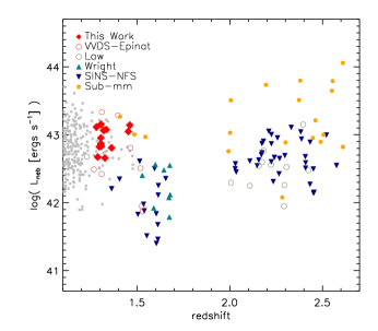
Figure 1: Nebular luminosity as a function of redshift for the largest high-redshift IFS surveys with the work presented here shown by the red diamonds. The gray points show the [O II] luminosity of other WiggleZ galaxies considered for this sample. The red circles show the sample from Epinat et al. (2009) taken from the VVDS survey and observed with SINFONI on the VLT. The green circles show the sample from Law et al. (2009) observed with OSIRIS on Keck. The blue inverted triangles show the SINS sample from Förster Schreiber et al. (2009) observed with SINFONI, and the green triangles show the sample from Wright et al. (2009) observed with OSIRIS. The orange points are SMGs with measured H$\alpha$ taken from Swinbank et al. (2004) and Takata et al. (2006).

In this paper, we present 13 galaxies and their physical properties. In Section 2 we describe our sample selection, observational technique, and data reduction methods. In Section 3 we discuss the properties of the galaxies, in particular we describe the morphological and kinematic properties. In Section 3.6 and 3.7 we discuss the methods of disk fitting and surface brightness profile fitting analysis. The individual and global properties of the 13 systems described in Section 3 are analyzed in Section 4 in the context of theories of galaxy formation at high redshift and the implications for the mechanism triggering massive rates of star formation. We conclude with a summary of our results and interpretations in Section 5, giving a brief list of the key points presented in this paper. The properties of the 13 individual galaxies are described individually in the Appendix.

A standard $\Lambda$CDM cosmology of $\Omega_{\mathrm{m}}=0.3$, $\Omega_{\Lambda}=0.7$, $h=0.7$ is adopted throughout this paper (e.g. Komatsu et al. 2011). In this cosmology, at redshift $z=1.3$, 1 arcsec corresponds to 8.38 kpc.

2 Observations

2.1 Target Selection

Our sample of 13 galaxies was selected from the WiggleZ Dark Energy Survey (Drinkwater et al., 2010). WiggleZ is a UV-selected survey of 238,770 unique emission line galaxies in the redshift range $0<z<1.5$, measured over 245 nights with the AAOmega spectrograph (Sharp et al., 2006) on the 3.9-m Anglo-Australian Telescope (AAT). The primary aim of the survey is to precisely measure the scale of baryon acoustic oscillations imprinted on the spatial distribution of these galaxies at look-back times of 4–8 Gyrs (Blake et al., 2011). The survey samples a total volume of $\sim$1 Gpc³ over 816 deg² of sky across seven fields, with an average target density of 350 galaxies per deg². Photometric data used in target selection for the WiggleZ survey are from the the Galaxy Evolution Explorer (GALEX) satellite (Martin et al., 2005), the fourth data release of the Sloan Digital Sky Survey (SDSS; Adelman-McCarthy et al. 2006) in the northern galactic region, and the Canada-France-Hawaii Telescope Second Red-sequence Cluster Survey (RCS2; Gilbank et al. (2011)) in the southern galactic region.

Whilst the WiggleZ galaxy redshift distribution peaks at $z\sim 0.6$ a long thin tail of high-redshift galaxies reaches to $z=1.5$. These high-redshift galaxies are identified by strong [O II] emission lines, with the [O II] doublet marginally resolved, and have star formation rates of $>50$M_⊙ yr^-1.

Galaxies selected for this study were drawn from the WiggleZ survey subject to a variety of criteria. Primary selection required (1) redshifts of $1.2<z<1.5$, where the [O II] emission line falls between OH sky residuals at $\sim$8000–10000 Å, and (2) [O II] emission exceeding $50\times 10^{-15}$ ergs s^-1 cm^-2. We found $\sim$300 targets in the WiggleZ survey that satisfied the aforementioned criteria. To reduce contamination from active galactic nuclei (AGN), starbursts were preferentially selected by (3) omitting galaxies with [Mg II] emission visible in the WiggleZ spectrum which may be indicative of AGN activity (Grandi & Phillips, 1979). With the additional criteria the number of targets was reduced to $\sim$100 galaxies. Finally, for IFU observations with laser guide star adaptive optics (LGSAO), a suitable tip-tilt star is required to correct aberrations in the wavefront. We require a star with apparent r-band magnitude $m_{\mathrm{r}}\la 17$ with an angular separation $<60$ arcsec from the science target for optimal acquisition. This last criteria reduced our final target sample to $\sim$50 targets.

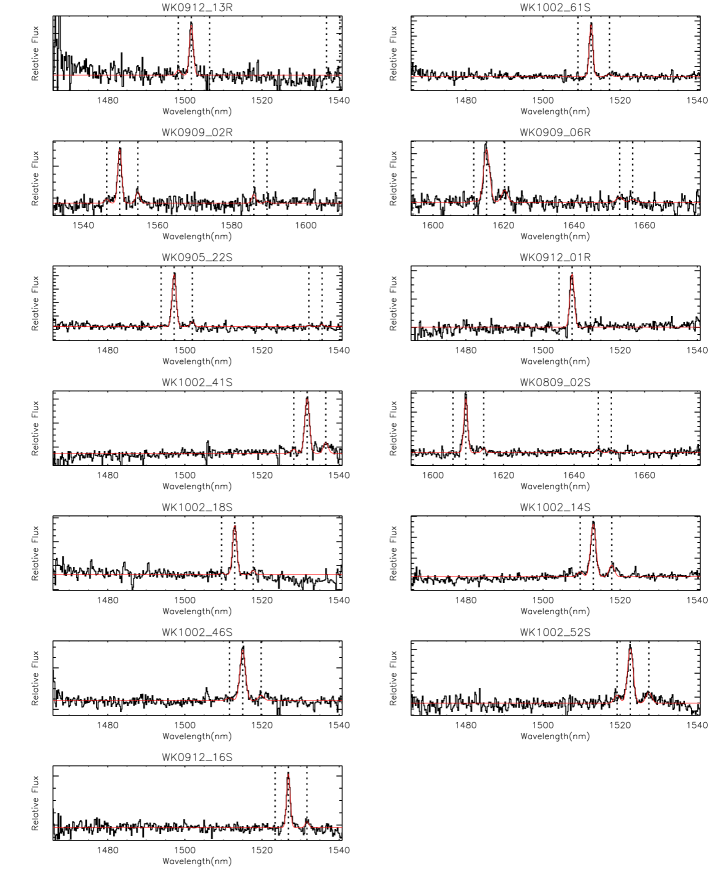
Figure 2: OSIRIS integrated spectra of each galaxy over all pixels satisfying the criteria outlined in Section 2. The vertical dotted lines denote the position of the redshifted locations of nebular emission lines: H$\alpha$, [N II]$\lambda$$\lambda$6548, 6584, and [S II]$\lambda$$\lambda$6716, 6731 at the systematic redshift. The solid red line is the best-fitting single Gaussian fits to each detected emission line.

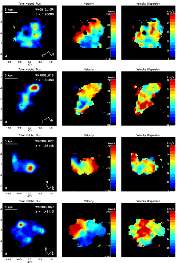
Figure 3: OSIRIS H$\alpha$ kinematics. Left: H$\alpha$ flux map, middle: velocity map from the systemic velocity, right: velocity dispersion map. The black crosses mark the peak(s) in H$\alpha$ flux. Velocity shifts from the systemic redshift and velocity dispersion are measured in km s^-1. Compass at the bottom right of the left panels show the true orientation. Letters at the bottom left of the left panels represent morphology classifications; M=Multiple emission, E=Extended emission, S=Single emission. Objects are presented in the order based on the morphological classification described in Section 3.1.

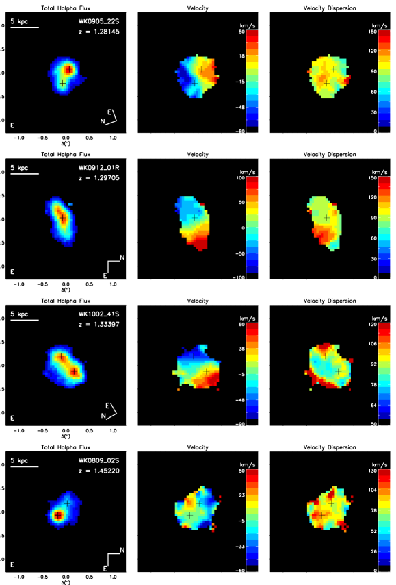
Figure 3: cont.

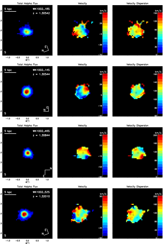
Figure 3: cont.

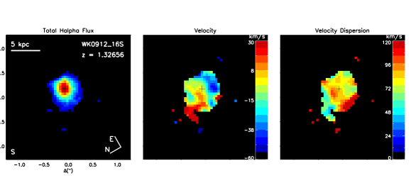
Figure 3: cont.

Table 2: Emission Line Properties

WiggleZ ID	ID	$z_{\mathrm{sys}}^{a}$	$f_{\mathrm{H\alpha}}^{b}$	$f_{\mathrm{[N\hskip 0.85355ptII]}}^{b}$	$L_{\mathrm{H\alpha}}$	$12+\mathrm{log}$(O/H)
					(1041 ergs s-1)
R03J032450240$-$13550943	WK0912_13R	1.2873	48 $\pm$ 16.1	$<$8.4	46.8 $\pm$ 13.2	$<$8.47
S15J145355248$-$00320351	WK1002_61S	1.3039	81.5 $\pm$ 5.3	$<$9.4	81.9 $\pm$ 13.7	$<$8.37
R01J005822757$-$03034040	WK0909_02R	1.3616	41.5 $\pm$ 7.9	9.3 $\pm$ 4.4	46.4 $\pm$ 15.2	8.53 $\pm$ 0.29
R03J032206214$-$15443471	WK0909_06R	1.4602	94.9 $\pm$ 6.7	22.8 $\pm$ 3.7	126.2 $\pm$ 18.1	8.55 $\pm$ 0.1
S15J144102444+05480354	WK0905_22S	1.2810	105.4 $\pm$ 4.3	10.8 $\pm$ 2.3	101.4 $\pm$ 13.1	8.34 $\pm$ 0.12
R00J232217805$-$05473356	WK0912_01R	1.2960	57.3 $\pm$ 7.5	$<$6.4	56.7 $\pm$ 13.5	$<$8.36
S09J091517481+00033557	WK1002_41S	1.3330	64.9 $\pm$ 4.3	13.7 $\pm$ 2.4	68.9 $\pm$ 14.4	8.52 $\pm$ 0.1
S00J233338383$-$01040629	WK0809_02S	1.4521	74.7 $\pm$ 13.6	6.3 $\pm$ 7.3	98.0 $\pm$ 17.8	8.29 $\pm$ 0.68
S15J142538641+00483135	WK1002_18S	1.3044	58.0 $\pm$ 4.8	$<$7.6	58.4 $\pm$ 13.7	$<$8.4
S11J101757445$-$00244002	WK1002_14S	1.3048	92.8 $\pm$ 4.3	20.6 $\pm$ 2.4	93.5 $\pm$ 13.7	8.53 $\pm$ 0.07
S09J090933680+01074587	WK1003_46S	1.3074	50.0 $\pm$ 4.5	$<$5.6	50.6 $\pm$ 13.8	$<$8.36
S11J110405504+01185565	WK1003_52S	1.3191	86.1 $\pm$ 6.0	20.4 $\pm$ 3.4	89.0 $\pm$ 14.1	8.54 $\pm$ 0.1
S09J090312056$-$00273273	WK0912_16S	1.3260	38.6 $\pm$ 4.4	7.5 $\pm$ 2.4	40.5 $\pm$ 14.3	8.49 $\pm$ 0.19

^aSystematic redshift measured from Gaussian fit to H$\alpha$ emission in integrated spectrum.

^bEmission line flux in units of 10^-17 ergs s^-1 cm^-2.

2.2 OSIRIS Observations

Out of the possible targets, spanning across seven fields, we observed 17 star-forming galaxies with OSIRIS (OH Suppressing InfraRed Imaging Spectrograph; Larkin et al. 2006) with the Keck II LGSAO system (Wizinowich et al., 2006; van Dam et al., 2006). These 17 targets were prioritized for having the brightest tip-tilt stars with shortest separation, and for which [O II] and H$\alpha$ fall fortuitously in clean sky regions. OSIRIS is a lenslet array spectrograph with a $2048\times 2048$ Hawaii-2 detector and spectral resolution $R\sim 3600$. Observations were performed in September 2008, May, September, and December 2009, and March 2010. The filters Hn1, Hn2, and Hn3 were used with central wavelengths of 1.500, 1.569, 1.635 $\mu$m respectively in the 0.05^′′ pixel scale. The FWHM of the tip-tilt stars ranged from one and a half to two pixels, 0.062-0.1^′′, with an average Strehl of 30% estimated from the tip-tilt stars. Seeing ranged from 0.4^′′ to 1.4^′′. The galaxies observed on these nights are listed in Table LABEL:osirisobs.table.

The standard observing procedure was as follows. We first acquired the tip-tilt star and applied the optimal position angle of OSIRIS to position the star within the un-vignetted field-of-view of the LGSAO system. Short, $60$s, integrations were taken on the star for calculations of the PSF and to centre the star in the field. A blind offset was then applied to the telescope to acquire the target. The WiggleZ survey selected targets from SDSS and RCS2 which follow different astrometry systems (Drinkwater et al., 2010). In calculating offsets from the reference star to the target, 2MASS (Skrutskie et al., 2006) and USNO-B (Monet et al., 2003) coordinates were used for SDSS and RCS2 galaxies respectively. The typical science observing sequence was to expose on target for 900s in each of two nod positions, A and B, separated by 1.6^′′ on the detector. If H$\alpha$ emission was detected in the difference of the first two exposures, we continued to expose on the galaxy for $\sim 1-2$ hrs as necessary to achieve a high signal-to-noise detection. Multiple A and B positions were dithered by $0.05^{\prime\prime}$ around the base positions in each exposure to remove bad pixels and cosmic ray contamination. Of the 17 observed targets, H$\alpha$ was detected in the spectra of 15 targets. The two non-detections were a result of the [O III]$\lambda$5007 emission line being mis-identified as [O II]$\lambda$3727 in the WiggleZ spectrum. Of the 15 detected targets, observations for two galaxies are unusable for scientific reduction due to poor AO correction as a result of stray light on the low bandwidth wavefront sensor. The H$\alpha$ luminosities of the final 13 galaxies are shown in Figure 1 with [O II] luminosities of all possible targets indicated by the small gray filled circles.

Data reduction was completed with the OSIRIS data reduction pipeline versions 2.2 and 2.3 and custom IDL routines developed for faint emission-line spectra. The pipeline removes crosstalk, detector glitches, and cosmic rays before it mosaics individual exposures and assembles a reduced data cube with two spatial and one wavelength dimension. First-order sky subtraction was achieved by the spatial ABBA nodding on the sky. Further sky subtraction was applied using custom IDL routines which employ the sky subtraction methods of Davies (2007). Galaxies were flux calibrated using telluric standard stars observed throughout the night. On average three telluric standards were observed each night.

Table 3: IRIS2 Observations of WiggleZ Galaxies

ID	Obs.	J Exp.	K Exp.	Ja	Ka
	Date	time(s)	time(s)
WK0912_13R	2010/01	1350	4050	20.71	20.13
WK0909_06R	2010/01	2700	3360	20.77	19.98
WK0905_22S	2009/05	1350	1350	21.36	20.52
WK1002_41S	2010/01	1350	3600	21.30	20.57
WK0809_02S	2010/07	1950	$\ldots$	20.66	$\ldots$
WK1002_18S	2009/05	1350	2700	20.84	21.02
WK1002_14S	2009/05	1350	1350	20.69	20.20
WK1002_52S	2010/01	1350	3300	19.94	18.92
WK0912_16S	2010/01	1260	4050	21.79	21.93
aApparent AB magnitudes. The average error on J and K
magnitudes are 0.11

2.3 Kinematic Mapping

In order to create 2-D spatial and kinematic maps of the H$\alpha$ emission line, the sky-subtracted data cube was convolved with a Gaussian kernel with $FWHM=150$ mas (200 mas in cases of low signal) to achieve a higher signal-to-noise ratio in each spaxel. A Gaussian profile was then fitted to the H$\alpha$ emission in each spaxel of the cube with the wavelength, intensity and width as free parameters. Errors were calculated by adding in quadrature an estimation of the sky noise from the variance of the spectrum offset from the emission lines with the Poisson error of the photon counting statistics in the emission lines. Spaxels were masked from the H$\alpha$ emission map and kinematic maps if the peak of the fitted Gaussian was less than one standard deviation above the median of the spectrum (corresponding to minimum signal-to-noise of $\sim$2), or the width of the Gaussian was less than the resolving power of the instrument. For spaxels surviving these cuts a flux was calculated from the fitted Gaussian. The H$\alpha$ flux images represent this array of fluxes. The integrated spectra, shown in Figure 2, were created by summing all unmasked spaxels in the spatial directions. A Gaussian was fitted to the observed-frame integrated spectrum to obtain the total H$\alpha$ flux and the systematic redshift, $z_{\mathrm{sys}}$ given in Table LABEL:flux.table. A velocity map was constructed for each galaxy using the velocity shifts of the emission line in each spaxel relative to $z_{\mathrm{sys}}$. The velocity dispersion was measured in each spaxel from the r.m.s. of the fitted Gaussian line profile corrected for instrumental broadening. All kinematic maps are shown in Figure 3.

2.4 NIRSPEC Observations & Data Reduction

When the Keck LGSAO system was unavailable due to bad weather, technical faults or space events, observations of available targets were taken with the near-infrared echelle spectrograph (NIRSPEC; McLean et al. 1998) to measure the $H\beta$ and [O III] emission line ratio. The ratios of emission lines from these observations, obtained for $WK0905\_22S$, $WK1002\_18S$, $WK1002\_52S$, $WK1002\_61S$, are used to constrain their AGN contamination as discussed in Section 3.4.

The NIRSPEC detector is a 1024$\times$1024 ALADDIN-3 InSb detector with spectral resolution $R\sim 2000$. All observations were carried out in February 2010 with the 4-pixel slit (42$\times$0.76^′′) in the NIRSPEC-2 filter (1.089$-$1.293 $\mu$m). Seeing in K was 0.8^′′ on average.

The typical observing sequence was to acquire a guide star, typically the star already selected for use with OSIRIS LGSAO system. Short ($\sim$10s) images were taken with the NIRSPEC guider to center the star at the central position on the slit. Once centered a blind offset was applied to the star position. Longer images were taken ($2\times 20$s) at the target position. If the target was observed in these images it was centered on the slit by nudging the slit left and right in single pixel intervals. Once centered spectroscopic object exposures were taken with typical sequence of $2\times 600$s in each of two nod positions, A and B in the sequence ABBA. Occasional shifts of a few pixels were needed to keep the object on the slit throughout the object exposures. No continuum was detected and the ratio of [O III]$\lambda 5007$/H$\beta$$\lambda 4861$ was calculated from the raw data.

Table 4: H$\alpha$ Kinematic & Morphological Properties

ID	$v_{\mathrm{shear}}^{a}$	$\sigma_{\mathrm{mean}}^{b}$	$\sigma_{\mathrm{net}}^{c}$	$v_{\mathrm{shear}}$/ $\sigma_{\mathrm{mean}}$	$r_{1/2}^{d}$	Classe
	(km s-1)	(km s-1)	(km s-1)		(kpc)
WK0912_13R	130.5 $\pm$ 11.0	81.6 $\pm$ 27.7	104.3 $\pm$ 27.1	1.6 $\pm$ 0.6	3.8	M
WK1002_61S	71.5 $\pm$ 10.7	85.1 $\pm$ 20.3	88.4 $\pm$ 4.4	0.9 $\pm$ 0.2	3.8	M
WK0909_02R	136.4 $\pm$ 6.1	87.9 $\pm$ 21.9	103.7 $\pm$ 15.5	1 $\pm$ 0.3	2.6	M
WK0909_06R	160.8 $\pm$ 2.4	92.6 $\pm$ 27.8	153.3 $\pm$ 8.4	1.6 $\pm$ 0.5	4.2	M
WK0905_22S	55.5 $\pm$ 6.5	98.2 $\pm$ 10.9	107.4 $\pm$ 3.3	0.6 $\pm$ 0.1	2.3	E
WK0912_01R	99.4 $\pm$ 7.1	98.6 $\pm$ 19.6	112.1 $\pm$ 11.0	1.3 $\pm$ 0.3	2.8	E
WK1002_41S	80.2 $\pm$ 5.4	91.4 $\pm$ 13.0	116.3 $\pm$ 5.9	1.7 $\pm$ 0.3	3.1	E
WK0809_02S	48.5 $\pm$ 9.4	92.7 $\pm$ 16.6	97.6 $\pm$ 13.8	0.4 $\pm$ 0.1	2.1	E
WK1002_18S	81.1 $\pm$ 17.5	102.1 $\pm$ 20.0	106.6 $\pm$ 6.8	0.7 $\pm$ 0.2	2.1	S
WK1002_14S	48.4 $\pm$ 9.5	113.7 $\pm$ 8.8	133.3 $\pm$ 4.8	0.5 $\pm$ 0.09	2.1	S
WK1003_46S	65.6 $\pm$ 16.7	124.8 $\pm$ 24.9	138.6 $\pm$ 9.6	0.5 $\pm$ 0.2	1.8	S
WK1003_52S	73.7 $\pm$ 18.2	125.4 $\pm$ 20.9	145.4 $\pm$ 8.1	0.7 $\pm$ 0.2	1.8	S
WK0912_16S	54.9 $\pm$ 12.9	85.1 $\pm$ 18.6	104.4 $\pm$ 9.1	0.7 $\pm$ 0.2	2.5	S

^aVelocity shear measured across the H$\alpha$ velocity map as described in Section 3.2.

^bFlux-weighted mean velocity dispersion calculated from a Gaussian fit to the spectra of individual spaxels of the OSIRIS H$\alpha$ detection.

^cVelocity dispersion calculated from a Gaussian fit to the integrated spectrum of the OSIRIS H$\alpha$ detection.

^dHalf-light radius of OSIRIS H$\alpha$ emission in circular aperture.

^eMorphological classification; E:Extended emission, M:Multiple emission, S:Single emission.

2.5 IRIS2 Observations

Near-infrared imaging was obtained for 9 out of 13 galaxies in the sample with the Infrared Imager and Spectrograph (IRIS2, Tinney et al. 2004) on the Anglo-Australian Telescope (AAT). $J$ and $Ks$ bands, with central wavelengths $\lambda_{c}=1.245~{}\mu$m and $\lambda_{c}=2.1444~{}\mu$m respectively, were chosen in order to image the older stellar population of each galaxy to obtain robust estimates of stellar masses. The IRIS2 detector is a $1024\times 1024$ Rockwell HAWAII-1 HgCdTe infrared detector, with a scale of 0.4487 arcsec pixel^-1 and field of view of 7.7 arcmin². Observations were carried out during May 2009, January 2010, and July 2010. Seeing in $Ks$ ranged between 0.9^′′-2.5^′′, 0.9^′′-1.6^′′, and 1.3^′′-2.0^′′, respectively.

The typical $J$ exposure sequence was a series of $15$ second exposures totaling $1350$ seconds on the target. The typical $Ks$ exposure sequence was a series of $10$ seconds exposures totaling $1350$ seconds on target. Most galaxies required 2 or 3 sequences in $Ks$ in order to obtain a detection with a signal-to-noise ratio greater than 5. Due to the time-sensitive variation of the infrared night sky, we used a dithering strategy of successive observations with 9 dithers per sequence with a maximum dither length of 20 arcsec.

Data reduction and mosaicking was carried out by data reduction pipeline ORAC-DR (Cavanagh et al., 2003). Each image was flattened with the other images closest in time and position in the dither pattern. The dithering script averaged out bad pixels on the detector and applied a nearest neighbor smoothing.

Magnitudes were calculated in the AB system using aperture photometry with a circular aperture of $4^{\prime\prime}$ with a concentric sky annulus. A zero point was derived for each reduced mosaicked image by comparing the measured aperture counts with known 2MASS magnitudes for several stars in the image. The zero point was then used to photometrically calibrate the image. On average, four uncrowded central stars with $K$-band magnitudes of $K\sim 15$ were selected to derive the zero point. If the standard deviation of the zero points from these stars was greater than 0.3, the stars producing the most deviant zero points were replaced with other stars in the field. Errors were calculated from the variance in the sky aperture. The sky background was calculated using a clipped mean. The IRIS2 system most closely resembles the Mauna Kea Observatory (MKO) system. Equations 1 and 2 were used to transform between the MKO and 2MASS systems,

$$J_{MKO} = -0.03-0.03\times(J-Ks)+J$$ (1)

$$K_{MKO} = -0.01-0.01\times(J-Ks)+K$$ (2)

where $J$ and $Ks$ are given in the 2MASS system and $J_{MKO}$ and $K_{MKO}$ are given in the Mauna Kea Observatory system used by IRIS2. Derived values of $J$ and $K$-band magnitudes are given in Table 3.

2.6 Stellar Mass Fitting

Stellar masses and star formation rates were calculated using an spectral energy distribution (SED) fitting routine (Glazebrook et al., 2004) which employs the Baldry & Glazebrook initial mass function (IMF) (BG03; Baldry & Glazebrook 2003). The BG03 IMF fits local cosmic luminosity densities well, with a high-mass slope similar to the classical Salpeter IMF but with a more realistic break at 0.5M_⊙. Hopkins & Beacom (2006) have shown that the BG03 IMF gives a better agreement between cosmic star-formation histories and mass assembly.

Infrared JK data from IRIS2 was combined with multiband photometry available in WiggleZ fields, including ugriz from SDSS, grz from the RCS2 Survey, and NUV from GALEX. Two-component modeling was adopted (using PEGASE.2 from Fioc & Rocca-Volmerange (1997) to calculate spectra) to assess the possible biases from starbursts on the calculated masses and to allow a range of dust extinction (0 $\leq A_{V}\leq$ 2 mag) and metallicity (0.0004 $\leq Z\leq$ 0.02). The primary component was modeled using SFR $\propto$ exp(-t/$\tau$) with $\tau=$0.1, 0.2, 0.5, 1, 2, 4, 8, & 500 Gyr (the first approximates an instantaneous starburst and the last a constant SFR). The full distribution function of allowed masses was calculated by Monte-Carlo re-sampling of the photometric errors. The final masses and error bars, given in Table 5, represent the mean and standard deviation of this full distribution function. In the cases where observed UV, optical and NIR magnitudes were available the errors in the derived stellar masses are on average $\delta$[log(M_∗[M_⊙])] = 0.15. When NIR magnitudes were not available, the errors average $\delta$[log(M_∗[M_⊙])]= 0.62.

We do not use the models of Maraston et al. (2006) as Kriek et al. (2010) show a low contribution from TP-AGB stars for post-starburst galaxies at high redshift. For more information on the SED fitting see Glazebrook et al. (2004).

Table 5: Stellar Properties

ID	log$[M_{*}(\hbox{M${}_{\odot}$})]$	$A_{V}$	SFRHα	SFR${}_{\mathrm{[O\hskip 0.85355ptII]}}^{a}$	SFRSED	SSFR
		(mag)	(M⊙ yr-1)	(M⊙ yr-1)	(M⊙ yr-1)	($10^{-9}\mathrm{yr}^{-1}$)
WK0912_13R	10.7 $\pm$ 0.2	1.1 $\pm$ 0.3	20.3 $\pm$ 6.8	43.3 $\pm$ 0.9	116 $\pm$ 40.4	1.8
WK1002_61S	10.7 $\pm$ 0.7	0.2 $\pm$ 0.2	35.6 $\pm$ 2.3	69.0 $\pm$ 2.8	25.6 $\pm$ 13	2.9
WK0909_02R	10.3 $\pm$ 0.6	0.7 $\pm$ 0.4	20.2 $\pm$ 3.8	33.1 $\pm$ 0.8	57.4 $\pm$ 41.5	4.6
WK0909_06R	11.0 $\pm$ 0.2	0.8 $\pm$ 0.3	54.8 $\pm$ 3.9	120.3 $\pm$ 14.9	91.8 $\pm$ 48.7	2.09
WK0905_22S	10.3 $\pm$ 0.2	0.3 $\pm$ 0.2	44.0 $\pm$ 1.8	202.4 $\pm$ 23.8	44.6 $\pm$ 15.1	10
WK0912_01R	10.0 $\pm$ 0.6	0.5 $\pm$ 0.2	24.6 $\pm$ 3.2	59.0 $\pm$ 3.8	40.3 $\pm$ 13	11.2
WK1002_41S	10.2 $\pm$ 0.1	0.4 $\pm$ 0.1	29.9 $\pm$ 2.0	112.8 $\pm$ 5.7	60.3 $\pm$ 9.3	8.1
WK0809_02S	11.1 $\pm$ 0.6	0.0 $\pm$ 0.1	42.5 $\pm$ 7.7	29.7 $\pm$ 0.8	19.5 $\pm$ 6.9	1.5
WK1002_18S	10.2 $\pm$ 0.1	0.5 $\pm$ 0.1	25.3 $\pm$ 2.1	188.6 $\pm$ 14.2	64 $\pm$ 17.4	6.09
WK1002_14S	10.6 $\pm$ 0.2	0.3 $\pm$ 0.1	40.6 $\pm$ 1.9	43.9 $\pm$ 0.7	55.5 $\pm$ 16	4.5
WK1003_46S	9.8 $\pm$ 0.6	0.2 $\pm$ 0.3	22.0 $\pm$ 2.0	41.3 $\pm$ 4.8	22.4 $\pm$ 17.1	12.8
WK1003_52S	11.7 $\pm$ 0.1	0.0 $\pm$ 0.1	38.6 $\pm$ 2.7	103.7 $\pm$ 16.9	15.9 $\pm$ 2.2	0.3
WK0912_16S	9.8 $\pm$ 0.2	0.1 $\pm$ 0.1	17.6 $\pm$ 2.0	64.1 $\pm$ 6.8	12.6 $\pm$ 3.2	12

^aErrors on the [O II]  SFRs are statistical errors only.

3 Results

In Figure 3 we present H$\alpha$ spatial (left panels) and kinematic maps of our 13 galaxies observed with OSIRIS with spatial extent ranging from $2-12$ kpc. A broad range of morphologies and kinematics are observed with 8/13 galaxies showing some velocity shear and the remaining showing disturbed kinematic morphologies (middle panels). The dispersion maps for the entire sample are chaotic with peaks in velocity dispersion exceeding $100$ km s^-1(right panels). In the next subsections we will discuss the H$\alpha$ morphology and kinematics, emission-line properties, and masses of the sample. For convenience IDs are shortened and referred to by their last three unique digits.

3.1 Classification

We initially classified the galaxies into three groups based solely on H$\alpha$ morphology: single emission, extended emission, and multiple emission. Galaxies classified as single-emission have a single resolved source of H$\alpha$ emission: 16S, 14S, 18S, 46S, 52S. Systems classified as extended emission show multiple unresolved or extended components: 02S, 22S, 01R, 41S. Systems 02R, 06R, 13R, 61S are classified as multiple-emission galaxies, which have multiple, resolved regions of H$\alpha$ emission. The centres of the separate components are marked in Figure 3. These classifications are made for the purpose of discussing properties of galaxies with similar morphologies. The classifications are used to order Tables and Figures. Kinematic classifications are discussed in Section 4.

3.2 Kinematic Quantities

A flux-weighted velocity dispersion ($\sigma_{\mathrm{mean}}$) was calculated from the dispersion and flux across all spaxels. We define velocity dispersion by $\sigma_{\mathrm{mean}}$,  which is representative of the internal motions of the gas (Law et al., 2007; Green et al., 2010). For comparison, a line-of-sight velocity dispersion ($\sigma_{\mathrm{net}}$) was calculated from the width of a Gaussian fit to the H$\alpha$ emission of the integrated spectrum. The measured values of $\sigma_{\mathrm{mean}}$ are consistent with or slightly less than $\sigma_{\mathrm{net}}$, as expected from velocity smearing. The values of $\sigma_{\mathrm{mean}}$  in this sample reach to $\sim 130$ km s^-1, and are typically higher than in the samples of Law et al. (2009) and Epinat et al. (2009). We note that the 0.15^′′ smoothing described in Section 2.3 produces a +10 km s^-1 median boost compared to $\sigma_{\mathrm{mean}}$ calculated from the non-smoothed data which is less than the statistical error. We give the $\sigma_{\mathrm{mean}}$ values from the smoothed data in Table 4 for comparison to the literature.

We do not make a correction based on beam smearing resultant from the PSF, which can be a problem for interpreting kinematic observations at high redshift (e.g. Law et al. 2009; Wright et al. 2009; Förster Schreiber et al. 2009; Epinat et al. 2010). Although all observations were taken in LGSAO mode, with a PSF of FWHM$\sim$850 pc, Law et al. (2009) and Wright et al. (2009) note that beam smearing can still have the effect of reducing the maximum rotation velocity and inflating the velocity dispersion for edge on disks in particular. However, as the inclination is not well constrained in this study it is unclear when and what correction would be appropriate. The same authors note that beam smearing does not explain the high velocity dispersions of objects which show no rotational velocity structure.

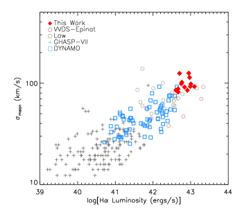
Figure 4: Flux weighted velocity dispersion as a function of $L_{H\alpha}$ from Green et al. (2010) with galaxies from this sample as red diamonds. The WiggleZ points extend this relationship to higher $\sigma_{\mathrm{mean}}$ and H$\alpha$ luminosity.

The observed dispersion and luminosity of the WiggleZ sample continues the relationship, spanning over $0<z<3$, observed by Green et al. (2010) for star-forming galaxies, recreated in Figure 4. The galaxies in the WiggleZ sample follow this relationship tightly with the highest dispersions and H$\alpha$ luminosities of the IFS samples introduced in Figure 1. Green et al. (2010) argue that the correlation seen implies star formation rate is the driving factor of the high velocity dispersion, not mass or gas fractions. Consequently, arguments that high velocity dispersions at high redshift are evidence for cold-flow accretion are weakened as the cold flows are no longer in place at the current epoch to produce the high dispersions observed in local galaxies.

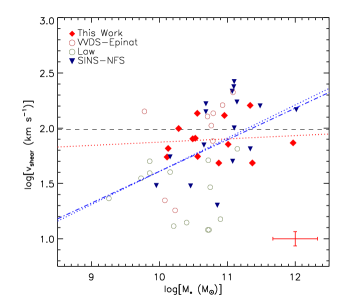
Figure 5: Logarithmic velocity shear as a function of logarithmic stellar mass for our 13 galaxies and galaxies from Law et al. (2009); Genzel et al. (2006, 2008); Förster Schreiber et al. (2006) and Epinat et al. (2009). Data are not corrected for inclination. All stellar masses are converted to the Salpeter IMF for ease of comparison with the literature. A median error for the WiggleZ points is plotted in red in the lower right corner. The red dotted line is the best-fitting linear model to the 13 galaxies in our sample [$\log$($v_{\mathrm{shear}}$ /km s^-1) $=0.03\times\log$(M_∗/M_⊙)$+1.58$]. The blue dot-dash line is the best-fitting linear model to the data from all the samples [$\log$($v_{\mathrm{shear}}$ /km s^-1) $=0.25\times\log$(M_∗/M_⊙)$-0.84$], the blue dotted line is the best-fitting linear model from Law et al. (2009) [$\log$($v_{\mathrm{shear}}$ /km s^-1) $=0.29\times\log$(M_∗/M_⊙)$-1.25$] and the black dashed line is at the value of $\langle\log$($\sigma_{\mathrm{mean}}$)$\rangle$.

A velocity shear was measured across each galaxy, $v_{\mathrm{shear}}=\frac{1}{2}(v_{\mathrm{max}}-v_{\mathrm{min}}),$ following Law et al. (2009). In order to prevent biasing from outliers, $v_{\mathrm{max}}$ and $v_{\mathrm{min}}$ are calculated from the mean of the highest and lowest 5% of the velocity map respectively (Gonçalves et al., 2010). The values of $v_{\mathrm{shear}}$ underestimate the true rotational velocity of the gas in the cases that the galaxy extends to greater radii than detected by OSIRIS. The values of $\sigma_{\mathrm{mean}}$, $\sigma_{\mathrm{net}}$, $v_{\mathrm{shear}}$, and $v_{\mathrm{shear}}$/$\sigma_{\mathrm{mean}}$ are given in Table 4. We do not find a correlation between velocity shear and stellar mass in this sample of 13 galaxies, in disagreement with the $z\sim 3$ sample of Law et al. (2009) and Lyman break analogs at $z\sim 0.1$ (Gonçalves et al., 2010). However, in the context of other star-forming galaxies at $1<z<3$ a positive correlation is seen, as shown in Figure 5. The interpretation of the relationship is that stable rotation is more prevalent in galaxies that have assembled a relatively large stellar population. However, the addition of this sample does not affect the correlation originally published by Law et al. (2009). It is unclear if the velocity shear from all samples are comparable given the different spatial scales probed by OSIRIS and SINFONI and the different signal-to-noise reached for each set of observations.

3.3 Star Formation Rate Indicators

Star formation rates were measured from WiggleZ [O II] and OSIRIS H$\alpha$ luminosities. Due to uncertainties arising in the flux calibration of optical fiber spectroscopy, the WiggleZ [O II] fluxes are only accurate to within 40% due to systematic errors. OSIRIS H$\alpha$ flux measurements are comparably more accurate and are thus used as the primary measure of the nebular star formation. Star formation rates (SFR) were calculated from Kennicutt (1998),

$$\mathrm{SFR}_{\mathrm{H}\alpha}[\mathrm{M}_{\odot}~{}\mathrm{yr}^{-1}]=\frac{1}{1.82}\frac{L_{\mathrm{H}\alpha}~{}[\mathrm{ergs~{}s}^{-1}]}{1.26\times 10^{41}}$$ (3)

$$\mathrm{SFR}_{\mathrm{OII}}[\mathrm{M}_{\odot}~{}\mathrm{yr}^{-1}]=\frac{1}{1.82}\frac{L_{\mathrm{OII}}~{}[\mathrm{ergs~{}s}^{-1}]}{7.1\times 10^{40}}$$ (4)

where the 1/1.82 converts to the BG03 IMF.

Further measurement of star formation is derived from the SEDs generated from the stellar mass fitting described in Section 2.5 (SFR_SED). A dust extinction, $Av_{\mathrm{SED}}$, is estimated from the SED fitting described in Section 2.6 and given in Table 5. The mean error on $Av_{\mathrm{SED}}$ is 0.2.

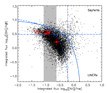
Figure 6: The emission line diagnostic diagram of Baldwin, Phillips & Terlevich (1981). The black points are WiggleZ galaxies and the red diamonds are 52S, 22S, 61S and 18S from this sample. The shaded gray area is the range containing the [N II]/H$\alpha$ ratio for the remainder of the systems in this sample. The dashed curved line is the empirical line from Kauffmann et al. (2003), the solid curved line is the theoretical curve from Kewley et al. (2001) and the vertical and horizontal lines are used to identify Seyferts and LINERS as labelled. The WiggleZ sub-sample presented here is primarily in the region of the diagram were star formation is the dominant mechanism driving line emission.

3.4 Metallicity

[N II] was detected in 8 of the 13 galaxies in our sample. The detections and upper limits are used to investigate the metallicity and level of contamination from hosting an AGN by using the [N II]$\lambda$6584/H$\alpha$ ratio. Metallicity was calculated from this ratio, as calibrated by Pettini & Pagel (2004),

$$12+\mathrm{log}(\frac{\mathrm{O}}{\mathrm{H}})=8.90+0.57\times\mathrm{log}(\frac{\mathrm{[N\hskip 0.85355ptII]}}{\mathrm{H}\alpha})$$ (5)

and given in Table LABEL:flux.table. The metallicities of the sample are all sub-solar and are consistent with the results of IFS samples at $z\sim 1-3$ of Genzel et al. (2008); Stark et al. (2008); Law et al. (2009); Förster Schreiber et al. (2009); Wright et al. (2009) and DEEP2 star-forming galaxies at $z\sim 1.3$ (Shapley et al., 2005). The typical errors in $12+\mathrm{log}(\frac{\mathrm{O}}{\mathrm{H}})$ are 0.2.

Metallicity measurements calculated from Equation 5 alone can be biased due to elevated levels of [N II] caused by AGN contamination. We look for this bias by constraining the position of the galaxies in this sample on the emission line diagnostic, or BPT, diagram (Baldwin, Phillips & Terlevich, 1981), shown in Figure 6. NIRSPEC observations of [O III]$\lambda$5007, 4959 and H$\beta$ of four galaxies in the sample further quantify AGN contamination using the [O III]$\lambda 5007$/H$\beta$ ratio. Two of the [N II]/H$\alpha$ measurements are upper limits (see column 5 of Table 2), and in all cases the [N II]/H$\alpha$ ratios are significantly lower than the level expected for the given values of [O III]$\lambda 5007$ / H$\beta$ if there was a significant component of AGN emission. The remainder of galaxies all lie to the left of $\log$([N II]/H$\alpha$) = $-0.6$, in the shaded gray region of Figure 6. Although AGN contamination can not be ruled out completely for these sources, their integrated nebular emission is clearly dominated by star formation.

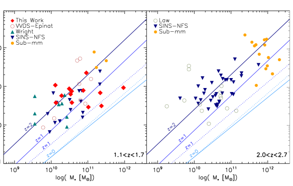
Figure 7: H$\alpha$ star formation rates of IFU samples at $z>1$ as a function of stellar mass. Stellar masses and SFRs for all samples are converted to the Salpeter IMF for ease of comparison to the literature. The symbols are as described in Figure 1. The solid lines are from the Great Observatories Origins Deep Survey (GOODS) given in Elbaz et al. (2007) and Daddi et al. (2007). The dotted lines are from the Millennium simulation(Springel et al., 2005; Croton et al., 2006) at redshifts $z=0$ (light blue) and $z=1$ (blue). An extinction correction is made from E(B$-$V)_SED.

3.5 Mass Estimates

The sample stellar masses range from $9.8<\log(\mathrm{M}_{*}[\hbox{M${}_{\odot}$}])<11.7$, comparable to masses from other IFS samples covering the same redshift range ($1.2<z<1.7$; Epinat et al. 2009; Wright et al. 2009; Förster Schreiber et al. 2009) but with a higher $\langle$M${}_{*}\rangle$ than high-redshift IFS samples ($z>2$; Law et al. 2009; Genzel et al. 2008). No correlation is found between H$\alpha$ morphology and mass; the three most massive systems cover all three morphological classes, and the three lowest-mass galaxies cover two morphological classes.

With stellar mass estimates we are able to identify where these systems lie relative to the main sequence of star formation (SFR vs. M_∗) as a function of redshift informing on the intensity of their star formation (e.g. Noeske et al. 2007; Rodighiero et al. 2010). If positioned above the main sequence, outside the limited range of SFRs at a given M_∗, the star formation of the sample may be indicative of episodic variations rather than being associated with the larger population of continuous star-forming galaxies. Furthermore, the main sequence evolves with redshift in which higher SFRs were more typical in past epochs. Rodighiero et al. (2010) show that the mean specific SFR (SSFR$\equiv$SFR/M_∗) of galaxies decreases by a factor of $\sim 15$ from $z=2$ to $z=0$ for the most massive galaxies. The main sequence for IFS samples is shown, as SFR vs M_∗, in Figure 7 in two redshift bins to account for this evolution. The SSFR is calculated, using SFR_Hα, and presented in Table 5.

In the lower-redshift bin of Figure 7, $1.2<z<1.7$, the star-forming galaxies of the SINS survey and Wright et al. (2009) form a sequence of star formation which scatter between the GOODS $z=1$ and $z=2$ empirical relations. The WiggleZ points in contrast do not show an increase in SFR with mass and therefore the galaxies in this sample below $\mathrm{M_{*}}=5\times 10^{10}$ M_⊙ scatter above the main sequence and the galaxies with masses $>5\times 10^{10}$ M_⊙ scatter below the main sequence. We note that the extinction correction applied here is derived from the SED fitting and future measurements of the dust content from far-infrared indicators will provide a more accurate correction affecting the location of this sample along the main sequence.

The high-redshift bin, $2.0<z<2.7$, shows a similar main sequence from the star-forming galaxies of the SINS Survey and Law et al. (2009) which scatters around the GOODS $z=2$ empirical relation. The mean SFR in the low-redshift bin ($\langle z\rangle\sim 1.52$) is a factor of 0.7 less than the the mean SFR in the high-redshift bin ($\langle z\rangle\sim 2.3$). Sub-millimeter galaxies (SMGs) are included in Figure 7 for comparison to the IFS samples. SMGs are considered as the ‘maximum starbursts’ (Tacconi et al., 2008) with infrared determined SFRs $>1000$ M_⊙ yr^-1. For consistency, only SMGs with published nebular emission are included in the comparison to IFS results (Swinbank et al., 2004; Takata et al., 2006). SMG stellar masses are taken from Michałowski et al. (2010). SFRs for all samples are calculated from measured nebular flux values with an extinction correction from $A_{\mathrm{V,SED}}$ and with a Salpeter IMF for consistency.

We find that the SMGs in the low-redshift bin are well matched statistically to the lower mass data presented here and higher on average than the other IFS samples. In the high-redshift bin the SMGs are offset in mass from the IFS samples. Unfortunately, the low number of SMGs with measured line emission limits an in-depth comparison to this interesting galaxy population. However, initial comparisons to the available data indicate the WiggleZ sample presented here may be related to SMGs with more episodic star formation than LBGs at a given redshift and stellar mass.

Figure 8: Disk fitting results for the 7/13 galaxies well-fit by disks in the sample. The first panel shows the smoothed velocity map, the second panel shows the smoothed modeled velocity map fit to the unsmoothed data, the third panel shows the residual from the difference of panel 1 and panel 2 and the final panel shows the binned rotation curve across the major axis with the model overlaid in red.

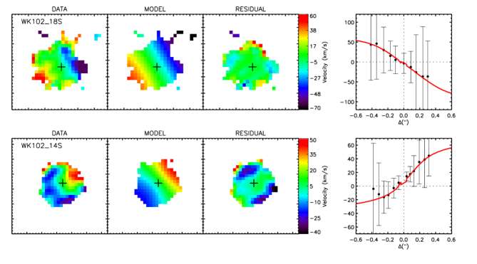
Figure 8: cont.

Table 6: Disk Model Parameter Results

ID	$\phi$	$V_{\mathrm{p}}\sin(i)$	$r_{\mathrm{p}}$	$V_{\mathrm{0}}$	Residual	$\chi^{2}_{\mathrm{R}}$
		(km s-1)	(kpc)	(km s-1)	(km s-1)
WK0912_13R	25${}^{+331}_{-14}$	73${}^{+64}_{-32}$	2${}^{+20}_{-1}$	8${}^{+14}_{-9}$	3.2	1.97
WK0909_06R	53$\pm$2	187$\pm$7	1$\pm$1	43${}^{+5}_{-6}$	4.3	5.12
WK0905_22S	287${}^{+10}_{-6}$	102${}^{+80}_{-26}$	5${}^{+3}_{-7}$	-7${}^{+32}_{-22}$	3.5	2.27
WK0912_01R	226${}^{+21}_{-35}$	83${}^{+49}_{-43}$	18${}^{+6}_{-3}$	-14${}^{+7}_{-8}$	2.6	3.44
WK1002_41S	219$\pm$14	141${}^{+126}_{-20}$	10${}^{+6}_{-2}$	-7${}^{+28}_{-26}$	1.5	0.99
WK1002_14Sa	320$\pm$36	42${}^{+49}_{-30}$	17${}^{+3}_{-17}$	15${}^{+6}_{-5}$	1.1	1.71
WK1002_18Sa	140${}^{+58}_{-65}$	24${}^{+32}_{-21}$	16${}^{+8}_{-3}$	28$\pm$7	2.1	2.58

^aKinematic center fixed to peak of H$\alpha$ flux distribution.

3.6 Disk Fitting

The velocity maps of the galaxies were modeled to determine whether the data are consistent with disks. Inclined disk models are generated varying the kinematic centre ($x_{\mathrm{0}},y_{\mathrm{0}}$), the inclination ($i$, where $i$=0 is a face-on disk), the position angle ($\phi$), the systemic velocity ($V_{\mathrm{0}}$), the plateau velocity ($V_{\mathrm{p}}$), and the plateau radius ($r_{\mathrm{p}}$) using the prescription of Begeman (1989),

$$V(x,y)=V_{\mathrm{0}}+V_{\mathrm{c}}(r)\sin(i)\cos(\theta),$$ (6)

where $V_{\mathrm{c}}$ is the circular velocity at a given radius from ($x_{\mathrm{0}},y_{\mathrm{0}}$) and $\theta$ is the azimuthal angle in the plane of the galaxy, defined as:

$$\cos(\theta)=\frac{-(x-x_{0})\sin(\phi)+(y-y_{0})\cos(\phi)}{r},$$

$$\sin(\theta)=\frac{-(x-x_{0})\cos(\phi)+(y-y_{0})\sin(\phi)}{r\cos(i)}.$$ (7)

The circular velocity is defined as:

$$V_{\mathrm{c}}(r)=\begin{cases}&V_{\mathrm{p}}\frac{r}{r_{\mathrm{p}}},\hskip 19.91684ptr\leq r_{\mathrm{p}}\\ &V_{\mathrm{p}},\hskip 28.45274ptr>r_{\mathrm{p}}\end{cases}$$ (8)

for a flat rotation curve (Wright et al., 2007). The ‘flat’ disk model has been shown statistically to reproduce fitting parameters more successfully than the exponential disc, isothermal sphere, and arctangent models in artificially redshifted IFS data (Epinat et al., 2010). The models are convolved with the observed PSF, modeled from a tip-tilt star observation, and are fit to the data prior to the 0.15^′′ smoothing to reduce the effects of beam smearing. The best-fitting models were determined by minimizing the reduced chi-squared value ($\chi^{2}_{\mathrm{R}}$) using Monte Carlo Markov Chain methods. The parameter results of the best-fitting models, $\chi^{2}_{\mathrm{R}}$ values, and the average residual velocity are given in Table 6. Example models are shown in Figure 8. The residual velocity, $v_{\mathrm{res}}$, is calculated from the pixel average of the absolute value of the difference of the data and model.

The kinematic center is not well constrained in single emission galaxies, particularly in the single emission galaxies that show no shear or have fewer spatial pixels. In these cases, specified in Table 4, the kinematic center is fixed to the peak of H$\alpha$ emission. Although the peak of H$\alpha$ emission is not necessarily the dynamical center of the galaxy, Wright et al. (2009) find that it is a reasonable approximation.

We find that 7/13 of our galaxies (06R, 01R, 13R, 41S, 22S, 14S, 18S) are well fit by a disk model. To determine which objects are well fit by this simple disk model we consider the velocity residual, reduced chi-square value and a qualitative measure of coherent velocity shear. We note that $\chi^{2}_{\mathrm{R}}$ is biased as the spaxels are correlated due to the intrinsic PSF and is not alone a reliable indicator. Furthermore, small fluctuations in the velocity map resulting from galactic winds and/or interactions between individual star-forming regions will inflate the residual and reduced chi-squared values as they are not accounted for in the model.

A known approximate degeneracy exists between $V_{\mathrm{p}}$ and $i$ in the form $V_{\mathrm{p}}\sin(i)$ in Equation 6 (e.g. Begeman 1989; Law et al. 2009; Epinat et al. 2009). In previous low signal-to-noise IFS work the inclination is set to a constant of $i=45$ (Wright et al., 2009) however, Law et al. (2009) derive $i=57.3$ as the correct average inclination between our line of sight to a given disk and the vector normal to the disk. The most robust method may be to fix the inclination to values derived from deep broadband imaging (Epinat et al., 2009), however we consider $V_{\mathrm{p}}\sin(i)$ as one parameter in this study as we lack sufficiently deep imaging to determine it from photometry.

We find another degeneracy present in 41S, 14S and 13R between the plateau radius and plateau velocity. This degeneracy arises from the linear nature of the velocity gradients observed and is likely a consequence of not probing to faint enough surface-brightness emission to detect the kinematic turnover. A characteristic peak of velocity dispersion, a result of rapid unresolved change in velocity, would not be expected in the dispersion maps. Similarly, face-on and low mass galaxies which have a low velocity gradient show a very faint or no central peak of velocity dispersion (Epinat et al., 2010). As a result we do not use the central peak of velocity dispersion as an indicator for disk classification.

As found in previous IFS studies of high-redshift galaxies the v_shear/$\sigma_{\mathrm{mean}}$ (Table 4) values of this sample are approximately unity. The $v/\sigma$ measurement is often used to make a split between rotationally supported systems ($v/\sigma>1$) and systems dominated by dispersion ($v/\sigma<1$). In this sample 02R, 06R, 01R, 13R have $v/\sigma>1$ while 02S, 22S, 16S, 46S, 52S have $v/\sigma<1$ and 41S, 18S, 61S have $v/\sigma\approx 1$ within the errors. This correlates with the results of disk modeling in which 06R, 01R, 13R and 41S are well fit by disks and 02S, 16S, 46S, 52S are not well fit by disks. However, this picture fails for 22S, 14S which are well fit by disks but have $v/\sigma<1$ and 02R which likely has an elevated $v/\sigma$ as a result of an outflow rather than from the signature of rotational support (See Appendix). It is likely that the discrepancy between these two methods is a result of the detection limit of the observations. The v_shear measurement probes only the inner star-forming regions of the galaxies and is not representative of the overall rotational velocity of the galaxy, thereby reducing the value of $v/\sigma$. Other factors are known to reduce the observed values of $v/\sigma$ such as the foreshortening due to the inclination by a factor of $\sin i$ (Law et al., 2009). Because the inclination values in this study are poorly constrained this correction is not applied. As a result, more weight is given to the results of disk modeling rather than $v/\sigma$ in classifying galaxies as being rotationally supported.

3.7 Surface Brightness Profiles

The effective radius was calculated by fitting convolved 1-D Sérsic models to the H$\alpha$ surface brightness profiles of single-emission galaxies. In order to fit model Sérsic profiles, the central spaxel of the galaxy or star-forming complex was first identified from the peak of the flux maps. The distance to the remaining spaxels was calculated from the central point assuming a circular profile, reducing the number of free parameters by setting the aspect ratio to unity and position angle to zero. Individual measurements are averaged in radial bins. The models were convolved with the PSF. The best-fitting Sérsic profile model was determined by minimizing the chi-squared value ($\chi^{2}$) with three free parameters, $n$, $r_{0}$, and $\Sigma_{0}$, where $n$ is the Sérsic index, $r_{0}$ is the effective radius and $\Sigma_{0}$ is the surface brightness at the effective radius. We assume this simple model as the inclination and position angle determined in Section 3.6 are not well constrained.

The fitted results are shown in Table 7 with $r_{\mathrm{eff}}$ ranging from $0.4$ kpc $<r_{\mathrm{eff}}<1.9$ kpc and $n$ ranging from $0.5<n<2.0$. An example model fit to the data is shown in Figure 9. It is not completely understood what the flux profile of H$\alpha$ emission reveals about the parent galaxy as Sérsic profiles are more commonly fit to broadband emission representative of continuum emission from continuous star formation (Sérsic, 1968). However, the SINS survey obtained deep rest-frame optical images of six irregular galaxies in their sample and found surprisingly good morphological agreement between H$\alpha$ and broadband images (Förster Schreiber et al., 2010). They find the Sérsic parameters of H$\alpha$ emission and $H$-band emission (rest-frame optical) are consistent for the six galaxies with a difference on average of 0.08 for the Sérsic index and agreement within 3% for $r_{\mathrm{eff}}$. The Sérsic indices are comparable to our H$\alpha$ results with $n<1$ in all cases however they find greater effective radii with $r_{\mathrm{eff}}>2$ kpc in all cases, most likely due to the coarser resolution from their non-AO corrected observations.

The fitting method described above is applied to available $r$-band images from RCS2 only, as galaxies are unresolved in SDSS images. The RCS2 images, taken in average seeing of 0.7^′′, are sufficient to fit Sérsic profiles to 3 of 13 systems of the sample. We obtain results in the range $0.2<n<1.0$. A direct comparison to the H$\alpha$ Sérsic parameters however is not possible as the only RCS2 data available is of extended or multiple emission galaxies. Deeper imaging of the whole sample is needed to reveal whether the underlying stellar population probed by the rest-frame optical for these galaxies follows the morphology of the H$\alpha$ emission.

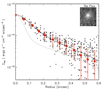
Figure 9: Example of surface brightness modeling results for 14S. The black points represent the flux in each spaxel from the peak of emission marked with the red plus sign in the H$\alpha$ image of the galaxy in the top right corner. The red circles represent binned points, the black solid line is the best-fitting Sérsic model, and the black dotted line is a fit to the flux profile of a tip-tilt star observed with OSIRIS.

Table 7: Surface Brightness Fitting

ID	n	$r_{\mathrm{eff}}$(kpc)
H$\alpha$ Images
WK0909_02R	$1.0^{+0.1}_{-1.6}$	0.6${}^{+0.2}_{-1.6}$
WK1002_18S	$0.8\pm 0.1$	$1.9\pm 0.4$
WK1002_14S	$0.9^{+0.03}_{-0.1}$	0.9${}^{+0.1}_{-0.2}$
WK1003_46S	$1.0\pm 0.1$	0.7${}^{+0.1}_{-0.2}$
WK1003_52S	$2.0^{+0.6}_{-0.1}$	$0.4\pm 0.1$
WK0912_16S	$0.5^{+0.1}_{-0.3}$	1.5${}^{+0.2}_{-0.6}$
RCS2 rest-frame UV Images
WK0912_13R	$0.6^{+0.1}_{-1.8}$	$4.6^{+2.9}_{-2.5}$
WK0909_02R	$1.0^{+0.2}_{-0.6}$	$6.1\pm 2.0$
WK0909_06R	$0.4\pm 0.3$	$3.4^{+2.6}_{-1.1}$

3.7.1 Radii

We note that radius is a particularly difficult property to measure robustly and consistently with a variety of methods used in the literature. We calculate the kinematic plateau radius, $r_{p}$, from disk modeling and the effective radius, $r_{\mathrm{eff}}$, from surface brightness profile fitting. The $r_{\mathrm{eff}}$ values presented are consistent with the sample of Law et al. (2009), $0.6$ kpc $\leq r\leq 1.6$ kpc, but are smaller than most other samples (e.g. Wright et al. 2009: $2.1$ kpc $\leq r\leq 3.9$ kpc, Förster Schreiber et al. 2009: $1.2$ kpc $\leq r\leq 7.5$ kpc, Epinat et al. 2009: $1.2$ kpc $\leq r\leq 5.5$ kpc). The half light radius, $r_{1/2}$, is also estimated directly from the data by determining the size of the circular aperture needed to enclose half the H$\alpha$ light from the centre of emission, and is given in Table 4. In some cases $r_{1/2}$ is the best measure of radius as neither $r_{\mathrm{eff}}$ or $r_{p}$ are able to be measured due to irregular morphologies and kinematics. The $r_{1/2}$ values are greater on average than the $r_{\mathrm{eff}}$, likely due to noise, and are comparable to the samples of Wright et al. (2009) and Epinat et al. (2009).

4 Discussion

The sample presented here was selected from the WiggleZ survey for strong UV and nebular luminosities. The luminosity, mass, SSFR, and $v_{\mathrm{shear}}$ are more comparable to the $z>2$ sub-set of the SINS survey than the samples at the same redshift, but more comparable in size to the $z\sim 2$ sample from Law et al. (2009). Like other IFS surveys we find a range of kinematics and morphologies with high velocity dispersions on average ($\langle\sigma_{\mathrm{mean}}\rangle=98$ km s^-1), yet the uniqueness of this sample is derived from the range of H$\alpha$ morphologies with resolved $kpc$-size star-forming regions and ultra-compact H$\alpha$ emission of the single emission galaxies.

However, IFS samples are all selected differently and may not be directly comparable. The SINS survey observes galaxies found from a variety of selection techniques including optical color selected ‘BX/BM’ galaxies (Steidel et al., 2004), infrared color selected ‘BzK’ galaxies (Daddi et al., 2004), Lyman break selected galaxies (LBGs), and bright sub-millimeter galaxies (SMGs). Epinat et al. (2009) select their galaxies from the magnitude complete VVDS survey, while Wright et al. (2009) observe BM galaxies, and Law et al. (2009) observed BX galaxies. While the WiggleZ sample was not selected by any of these methods, the SEDs of the sample imply that they could be classified as BM galaxies, BzKs and LBGs. Because IFS surveys are observationally expensive we are working with low number statistics and we cannot follow up mass or luminosity complete samples at high redshift.

The initial classification of this sample was based on H$\alpha$ morphology into three groups; single emission, extended emission, and multiple emission. A reclassification is now considered based upon the properties discussed in Section 3 in the context of disk formation at high redshift and a merger sequence. However, it is a challenge to distinguish between a galaxy merger and the merger of massive sub-clumps embedded within a rotating disk and similarly to distinguish between a merger remnant and a pseudo-bulge formed from the collapse of massive sub-clumps. Below we explore models of both disk formation and merger events at high redshift. We use the kinematic properties, masses, sizes, etc. to differentiate between the dominate formation mechanism for the WiggleZ galaxies sample presented here.

4.1 The Merger Hypothesis

With separations of 3–10 kpc the H$\alpha$ complexes may be sites of multiple regions of star formation merging from different parent galaxies. Kinematic quantities need to be utilized to find support for this hypothesis as deep imaging of diffuse continuum emission is unavailable to reveal tidal features characteristic of mergers. We analyze here a scenario in which our sample form a merger sequence with pre$-$, ongoing, and post$-$mergers.

In this scenario the multiple emission galaxies are the initial stages of mergers when star formation in separate galaxies can still be spatially differentiated. The extended emission galaxies are the next stage in the sequence representing ongoing merging activity (or pre-mergers with component confusion due to projection effects). The final stage in the proposed merger sequence is the single emission galaxies representing merger remnants with high dispersions and star formation rates.

Velocity dispersion maps provide some evidence indicating that we are seeing separate kinematic components merging. The observed peaks in dispersion may correspond to centres of individual galaxies or be a result of shock fronts between merging systems. Systems 41S and 61S show multiple peaks in velocity dispersion correlated with the brightest regions of emission, indicative that the system is an early-stage merger where each galaxy has a peak in velocity dispersion corresponding to an unresolved component. Systems 13R and 06R show multiple peaks in velocity dispersion correlated with the gas between the brightest regions of emission, indicative of the turbulence occurring from the interaction of the gas from the merging galaxies in this scenario or the effect of fitting substructure along the line of sight with a single Gaussian.

However, the majority of IFS results classified as mergers show velocity maps where the velocity does not vary smoothly across the source but rather show a quick turnover within a resolution element or less (Nesvadba et al., 2008; Wright et al., 2009; Law et al., 2009). An ideal example, presented in Nesvadba et al. (2008), is a merging system observed as two unresolved “clumps” of [O III] emission with a step in the velocity map between both components. This step function, observable with AO resolution, is not present in the kinematics presented here.

The single emission galaxies in this scenario could be merger remnants. This comparison is particularly difficult as merger remnants produced in simulations show a wide range of kinematic and morphological properties with observables sensitive to the initial mass ratio of the merger (Naab & Burkert, 2003). However, the majority of remnants are slow rotators (with v/$\sigma<1$), and have high velocity dispersions and minor axis rotation (Naab & Burkert, 2003; Cox et al., 2006; Bois et al., 2010). These properties could be used to describe 22S, 16S, 14S, 18S and 46S (although major and minor axes cannot be distinguished). These galaxies show some indication of rotation but with very low amplitudes ($v_{\mathrm{shear}}$  $\sim$40 km s^-1). But it is difficult to distinguish merger remnants and disks. Some simulations even find that a low percentage of remnants also have disk-like isophotes (Naab & Burkert, 2003).

A fraction of the sample, particularly the lower-mass galaxies, are found above the ‘main sequence’ of star formation (Figure 7), which indicates they may be undergoing a burst of star formation typical of a gas-poor or minor merger event (Noeske et al., 2007).

Unfortunately, surface brightness detection limits of OSIRIS may introduce a selection effect of detecting only the brightest objects in merging systems. This effect can be seen in Figure A1b of the Appendix for object 02R where an outflow or companion is seen in the RCS2 image but not detected in the H$\alpha$ OSIRIS image. Classification errors may arise as a result of this effect. Deep broadband imaging of all sources will help to reveal merging companions.

4.2 The Clumpy Disk Hypothesis

We investigate the scenario where the data presented here represent different stages of the clumpy disk models of the Elmegreen et al. (2008) simulations, hereafter EBE08. In this context galaxies with multiple regions of emission represent the early phases of disk formation when gravitational instabilities result in multiple star-forming complexes forming under Jeans collapse embedded within a disk galaxy. As turbulent speeds decrease relative to the rotational speed of the disk, the clumps migrate towards the centre on a timescale of 1 Gyr, represented here by the galaxies with extended emission. Finally, the clumps coalesce and form a slowly rotating pseudo bulge (Noguchi, 1999; Bournaud et al., 2007; Elmegreen et al., 2008; Dekel et al., 2009b; Krumholz & Dekel, 2010), represented here by galaxies with a single spherical emission profile.

The morphologies of multiple emission systems, 06R, 13R, and 61S (Figure 3) are well matched to the early stages of clumpy disk formation ($t=175-450$ Myr). Systems 06R and 13R are well fit by disk models. The clump velocities follow the global velocity structure of the galaxy as seen in Figure 8, where the major axis of rotation cuts across multiple clumps revealing no corresponding deviation in the rotation curves (Immeli et al., 2004b).

The morphologies of 02S, 22S, 41S and 01R are either consistent with the system being observed at the clump coalescence phase ($t=600-800$ Myr) or the result of projection effects. Systems 02S and 22S, each show two close components which can be distinguished when fitting surface brightness profiles, while 41S and 01R have single bright extended regions where multiple components cannot be differentiated visually or from surface brightness profiles. 22S, 41S and 01R are well fit by disk models whereas 02S has a flat velocity map with a peak in dispersion corresponding to the brightest peak in H$\alpha$ emission. The fainter peak of emission may be a signature of a galactic outflow resulting in confusion in classification.

Star-forming regions within a disk should have similar or consistent metallicities as they are evolving within the same conditions as predicted by theoretical models for disks at high redshift (Immeli et al., 2004a). In a major or minor merger no similar correlation is expected in the metallicities of each galaxy. By integrating the light of each clump, the clump metallicities are calculated from Equation 5. Metallicities of clumps in 06R and 61S are equal within the errors, as predicted for the early stages of disk fragmentation. At clump coalescence metallicities of individual clumps would be consistent as seen in 02S and 22S. Although this supports current theories, $12+\log$(O/H) varies little across the sample ($\Delta[12+\log$(O/H)]$\sim 0.26$).

Compact single emission galaxies 14S, 16S, 18S, 46S, and 52S have morphologies well matched to the later stage of simulated formation when the clumps have collapsed to form a bulge ($t=1000$ Myr). The dispersions of 14S, 46S, and 52S are the highest in the sample and are consistent with EBE08 bulges, predicted to form by clump coalescence and become slow rotators with high turbulence of $\sigma_{\mathrm{los}}\sim 130$ km s^-1 in their inner regions. Systems 14S, 16S, 18S all show velocity gradients with amplitudes less than 70 km s^-1. The bulge density profiles in the EBE08 models are well fit by Sérsic profiles of $n\sim 4$ in the inner 500 pc and $n>2$ at greater radii. While we do not resolve the inner 500 pc we do resolve to $650-750$ pc and find $n<2$ in all cases for the H$\alpha$ emission.

Velocity dispersion maps in this sample do not show characteristic central peaks in velocity dispersion observed in IFS studies in both local (de Zeeuw et al., 2002) and high redshift (Genzel et al., 2006; Förster Schreiber et al., 2009) disk galaxies and therefore cannot be used as an indicator for disk classification. As discussed in Section 3.6, this peak in velocity dispersion can be attributed to beam-smearing across the inner regions of the velocity turnover of the galaxy. However, because we are observing only the central region of rotation and have a small PSF as a result of using LGSAO, a dispersion peak is not expected.

Furthermore, if we model the velocity dispersion using the equation for a thick or compact disk (Binney & Tremaine, 2008);

$$\sigma\sim\frac{h_{\mathrm{z}}V_{\mathrm{c}}(r)}{r}$$ (9)

where $h_{\mathrm{z}}$ is the disk scale height, the expected model would give a constant, featureless dispersion map within the plateau radius ($r\leq r_{\mathrm{p}}$). This would be consistent with galaxies 41S, 14S, and 13R where a plateau velocity is never reached. In this case the observed variations in velocity dispersion are more likely a result of random perturbations within the centre of the disk or local perturbations due to clumps.

The simulations of EBE08 and others that model and evolve these galaxies have mainly been developed with sticky-particle codes (Elmegreen et al., 2008; Noguchi, 1999) which only model the cold gas associated with the cold cloud medium. Immeli et al. (2004a, b) do include a hot phase to their simulation allowing the galaxy models to track stellar ages and metallicities providing observables that can be tested. Furthermore, the initial conditions of such models require the disks to have very high velocity dispersions to mimic observational results at these redshifts making it difficult to distinguish inputs and outputs of the models. More realistic models are needed for a more rigorous comparison. Regardless of these limitations the data is well-matched to the available models.

5 Conclusion

We favor the clumpy disk model over the merger sequence model. We find 7/13 of the sample is well modeled by a disk and we find that clumps found in galaxies with multiple regions of emission do not strongly affect the kinematic fields. This provides observational evidence for the models of Elmegreen et al. (2008) which provide an explanation for the irregular morphologies seen at high redshift.

However, whilst natural to attempt to identify kinematic observations as disks or mergers, as been attempted here, this simplified picture of galaxies becomes increasingly fallible at high-redshift. More than half of the galaxy kinematics in this sample are well-described by disk models, however it is important to be cautious of definitive kinematic classifications. For example, Epinat et al. (2010) provide evidence that up to 30% of disk galaxies may be misclassified as perturbed rotators or complex kinematics with current classification schemes.

It is likely that we are seeing a variety of mechanisms at work which cannot be broken down into simply disks and mergers. Even if disk instability is a dominant mechanism in star-formation histories at high redshift, as we find here, the disks are still likely to undergo mergers in their lifetime further complicating kinematic interpretations. Lemoine-Busserolle et al. (2010), for example, observe a galaxy pair with separation of 12 kpc with one galaxy in the pair classified as a disk with velocity gradient of $\sim$91 km s^-1 and the other galaxy classified is compact and likely dominated by AGN. It is unclear how to classify this system, which has multiple kinematic components. Furthermore, With such small number statistics, the varying kinematics across multiple IFS samples could be due to varying properties amongst the galaxies selected and instruments used, making it difficult to compare results.

The global properties of the sample, the most luminous population, studied at $z\sim 1.3$ with IFS, are in surprising agreement with a model of unstable disks. We agree with Law et al. (2009) that statistically all high-redshift galaxies cannot be mergers. Models show that on average the enhancement of SFR in a merger is only a factor of a few and lasts $200-400$ Myr with peak enhancement lasting for less than 100 Myr (Teyssier et al., 2010; Di Matteo et al., 2008). It has been shown locally that all ultra-luminous infrared galaxies (ULIRGS) are mergers (Duc et al., 1997) and it is therefore possible a high-redshift subset of galaxies are also exclusively mergers. However, galaxies on average formed their stars more rapidly in the past implying the need for an evolving definition of what makes more luminous galaxies ‘extreme’. We therefore stress the importance of the bolometric luminosity in knowing if the sample presented here fall on or above the main sequence of star formation at this redshift to aid in making generalizations about galaxy populations at $z>1$.

Discerning the dust content will aid in a better understanding of their star-formation histories. Such moderate to high mass, gas rich, intensely luminous galaxies are reminiscent of local ULIRGs and $z\sim 2-3$ SMGs. However, critical to making this link is to determine their far-infrared and sub-mm SEDs, and enabling the measurement of their bolometric luminosities and dust content. Such quantities will inform on whether these galaxies are dust-enshrouded starbursts or dust-free late time proto-galaxies. We will present $Herschel$ data in a future paper that will address the dust content in this sample.

We expect to see signatures of outflows in these systems as galactic scale winds are expected in galaxies forming stars at $>5$M_⊙ yr^-1and are seen in 75% of ULIRGS (Veilleux et al., 2005). Previous studies have detected galactic winds with IFS (high-z: Swinbank et al. 2009; Alexander et al. 2010; Shapiro et al. 2009; local: Sharp & Bland-Hawthorn 2010). The high dispersions to the edges of 02S, 52S, and 02R are real and not an inflation from lower signal-to-noise data. This increase in dispersion towards the edges most likely indicates the presence of galactic winds which add an underlying broad component of H$\alpha$ (Veilleux et al., 2005). The influence of winds on this sample will be further discussed in a subsequent paper.

Measuring the properties of the individual clumps including size, metallicity, SFR, and velocity dispersion to compare to local samples will be important to testing models of clumpy disk formation. Only on order $\sim 10$ clumps have been resolved with IFS studies using lensing and a further $\sim 10$ resolved or marginally resolved within the SINS survey (Genzel et al., 2010). The properties of the 10 clumps identified in these systems will be presented in our next paper.

In this paper we:

• Present kinematic data of 13 star-forming galaxies at $z\sim 1.3$, selected from the WiggleZ Dark Energy Survey, of better or comparable resolution than previous studies.

• Extend the trend of Green et al. (2010) to higher star formation rates and higher dispersions between $1<z<2$ (Figure 4).

• Find the most luminous star-forming galaxies at this redshift show a variety of star-forming morphologies with a high incidence of star formation in disks.

• Identify clumps of 1–2 kpc in size at $z\sim 1.5$ that are resolved kinematically with LGSAO IFS without aid of lensing.

• Conclude the clumps in multiple emission galaxies follow the overall kinematics of the system, and find a high incidence of velocity gradients consistent with rotation lending support of the clumpy disk scenario of EBE08 over the major merger scenario.

Appendix A

A.1 Multiple Emission Galaxies

A.1.1 WK0912_13R

WK0912_13R has an extended irregular flux profile with faint surface brightness at the centre encircled by a brighter ring of emission. This galaxy shows multiple bright regions of H$\alpha$ spatial emission, however due to low signal the individual regions are not resolved. The velocity map shows an ordered velocity gradient with the“hole” in emission spatially placed at the central region of the velocity gradient and is well fit by a disk model. However, this detection has the lowest signal-to-noise of the sample and only a portion of the rotation curve is detected. Optical emission is shown in Figure 10.

Figure 10: RCS2 r-band and OSIRIS H$\alpha$ images for 02R, 01R, 06R, and 13R, the only objects with resolved broadband imaging. The green dot-dash lines on the RCS2 image of 02R mark the position of the LRIS long-slit. LRIS spectroscopy confirms the low surface brightness region below the central emission is at the same redshift as the central emission detected by OSIRIS.

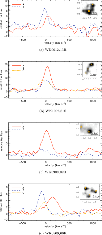
Figure 11: Integrated spectra from individual clumps for all multiple emission systems. Clumps and their corresponding spectra are labeled in H$\alpha$ images found in the upper right corner. The spectra are the integrated spectra of emission within 2 r_eff of star-forming regions that are resolved or marginally resolved.

A.1.2 WK1002_61S

The morphology of 61S reflects that of “chain galaxies” observed in the Hubble Ultra Deep Field (UDF) with $2-3$ resolved clumps marked by plus signs in Figure 3. However, unlike the clumpy galaxies 06R and 13R in this sample, 61S has one of the lowest velocity dispersions of this sample of $\sigma_{\mathrm{mean}}$=85 km s^-1 and shows little or no velocity separation between clumps as shown in Figure 11. There is a messy velocity gradient across the length of the “chain” with peaks of velocity dispersion spatially aligned with the peaks of the eastern most clumps.

A.1.3 WK0909_02R

WK0909_02R has the most irregular optical morphology of the objects with available broadband imaging. The RCS2 r-band image (0.185^′′/pixel) shows three distinct regions of emission spread over 4 arcseconds, including the central brightest region denoted by an $\times$ in Figure 10, a lower surface brightness feature to the NW, and a larger low surface brightness feature to the south of the brightest region extending $\sim$21 kpc away from the central peak of broadband emission. The OSIRIS observations of WK0909_02R has a single peak in H$\alpha$ flux with a faint tail of emission to the NW coincident with the peak of r-band emission and faint NW feature respectively. [N II]$\lambda\lambda$ 6584 is detected with peak flux coincident with peak H$\alpha$ flux. Long-slit spectroscopy with LRIS reveals the southern low surface brightness component is at the same redshift as the brighter central emission.

A.1.4 WK0909_06R

WK0909_06R has three resolved knots of H$\alpha$ emission. In velocity space these peaks correspond to a velocity range of approximately 320 km s^-1 shown in Figure 11. This large change in velocity over $\sim$10 kpc leads to broad velocity width of the H$\alpha$ emission line between flux peaks where a signature of two Gaussians is seen. Peak [N II] emission corresponds with the brightest peak of H$\alpha$ and is not detected elsewhere in the galaxy. Faint [S II] emission is detected in the integrated spectrum but does not have high enough signal-to-noise to be mapped spatially. The RCS2 image in Figure 10 reveals a possible optical companion 1.8^′′ to the south-west (15 kpc). Future long-slit spectroscopy will determine if the galaxies are under-going a merger.

A.2 Extended Emission Galaxies

A.2.1 WK0905_22S

The flux profile of WK0905_22S is also best fit by two components with the the primary peak of velocity dispersion occurring at the boundary of the two systems indicative of a line-of-sight merger, however the velocity map shows evidence of rotation and is well fit by a disk.

A.2.2 WK0912_01R

WK0912_01R has one extended peak of H$\alpha$ flux with a fainter surrounding halo. The velocity map shows a strong velocity gradient of $v_{\mathrm{shear}}$ $\sim 200$ km s^-1 and a near linear rotation curve. It is well-fit by a disk with optical morphology consistent with being an edge-on system as seen by the ellipticity of the rest-frame UV image in Figure 10. [N II]  was not detected in the OSIRIS observation of this galaxy, which is partly due to its short integration time, an upper limit is given in Table LABEL:flux.table.

A.2.3 WK1002_41S

The H$\alpha$ morphology of 41S reveals two peaks of emission connected by a dip in the H$\alpha$ surface brightness at the central region of the detection. The rotation profile of 41S is linear ($v_{\mathrm{shear}}$=114 km s^-1) with a featureless velocity dispersion; as a result there exist a strong degeneracy between $r_{\mathrm{p}}$ and $V_{\mathrm{p}}$ when fitting a disk profile. This indicates that 41S is well-fit by a disk but as we only detect the inner part of rotation, the kinematic extent cannot be constrained. It follows that the dispersion map is flat and featureless as the turnover has not been reached.

A.2.4 WK0809_02S

The 2-D flux profile of WK0809_02S is best fit by two emission components. The peak in velocity dispersion corresponds with the brightest peak in flux, however no clear velocity gradient is seen and the object has the lowest velocity shear in the sample ($v_{\mathrm{shear}}$ =36 km s^-1). With $J$ band photometry ($K$ not available) the stellar mass is estimated at $\log(\mathrm{M_{*}})$ = $11.1\pm 0.3$ M_⊙, one of the most massive of the sample. A tentative IRAM detection of the CO(2-1) emission line exists at 500 km s^-1 from the $z_{\mathrm{sys}}$ of H$\alpha$. The CO(2-1) line is formally 2.5$\sigma$ per channel, but spans $>$3 channels, so is $\sim$5$\sigma$ integrated over the line, possibly indicative of an outflow/inflow signature. This result is outside of the scope of this analysis and will be addressed in a subsequent paper.

A.3 Single Emission Galaxies

A.3.1 WK1002_18S

WK1002_18S is a compact resolved single emission galaxy with $n_{\mathrm{H}\alpha}$=0.8 and shows a near-linear velocity gradient. The stellar mass of 18S is $8\times 10^{9}$M_⊙and has a velocity dispersion $\sigma_{\mathrm{mean}}$$=102$ km s^-1.

A.3.2 WK1002_14S

WK1002_14S has a single compact region of resolved H$\alpha$ emission showing a linear velocity shear, with some variations in the velocity field at the edges of the galaxy detection. As with 41S there exists a degeneracy between $r_{\mathrm{p}}$ and $V_{\mathrm{p}}$ due to the linear nature of the velocity profile. The flat dispersion map can be explained by the lack of turn-over in the velocity profile. This galaxy is one of the highest dispersion galaxies with $\sigma_{\mathrm{mean}}$$\sim$130 km s^-1 and stellar mass of M_∗=$3.7\times 10^{10}$ M_⊙. [N II]$\lambda\lambda 6583.5$ is detected coincident with H$\alpha$ emission.

A.3.3 WK1002_46S

WK1002_46S is the most compact ( $r_{1/2}$(H$\alpha$)$\sim$1.8 kpc ) resolved galaxy. The stellar mass of 46S is $7\times 10^{9}$M_⊙and the galaxy has a relatively low $\sigma_{\mathrm{mean}}$$=85$ km s^-1.

A.3.4 WK1002_52S

52S is only marginally resolved and an outlier in many respects including: highest velocity dispersion ($\sigma_{\mathrm{mean}}$=125 km s^-1), highest stellar mass (M_∗=$4.6\times 10^{11}$ M_⊙), most compact ($r_{1/2}\sim$1.8 kpc). Given the high stellar mass it is more likely that 52S is a merger remnant rather than a newly forming bulge.

A.3.5 WK0912_16S

WK0912_16S is observed to have a single resolved peak in H$\alpha$ flux. [N II] is detected with peak flux coincident with the peak H$\alpha$ flux. 16S has one of the lowest velocity dispersions of the sample at $\sigma_{\mathrm{mean}}$$\sim 90$ km s^-1, and does not show a coherent velocity gradient. It also has the lowest stellar mass of the sample of $6.3\times 10^{9}$ M_⊙  and the flattest flux profile with $n_{\mathrm{H}\alpha}$=0.5${}^{+0.3}_{-0.1}$.

References

- Abraham et al. (1996) Abraham, R. G., Tanvir, N. R., Santiago, B. X., Ellis, R. S., Glazebrook, K., & van den Bergh, S. 1996, MNRAS, 279, L47
- Adelman-McCarthy et al. (2006) Adelman-McCarthy, J. K., et al. 2006, ApJS, 162, 38
- Alexander et al. (2010) Alexander, D. M., Swinbank, A. M., Smail, I., McDermid, R., & Nesvadba, N. P. H. 2010, MNRAS, 402, 2211
- Baldry & Glazebrook (2003) Baldry, I. K., & Glazebrook, K. 2003, ApJ, 593, 258
- Baldwin, Phillips & Terlevich (1981) Baldwin, J. A., Phillips, M. M., & Terlevich, R. 1981, PASP, 93, 5
- Begeman (1989) Begeman, K. G. 1989, A&A, 223, 47
- Binney & Tremaine (2008) Binney, J., & Tremaine, S. 2008, Galactic Dynamics: Second Edition, ed. Binney, J. & Tremaine, S. (Princeton University Press)
- Blake et al. (2011) Blake, C., et al. 2011, MNRAS,
- Bois et al. (2010) Bois, M., et al. 2010, MNRAS, 406, 2405
- Bournaud et al. (2007) Bournaud, F., Elmegreen, B. G., & Elmegreen, D. M. 2007, ApJ, 670, 237
- Cavanagh et al. (2003) Cavanagh, B., Hirst, P., Jenness, T., Economou, F., Currie, M. J., Todd, S., & Ryder, S. D. 2003, in Astronomical Society of the Pacific Conference Series, Vol. 295, Astronomical Data Analysis Software and Systems XII, ed. H. E. Payne, R. I. Jedrzejewski, & R. N. Hook, 237–+
- Conselice et al. (2003) Conselice, C. J., Bershady, M. A., Dickinson, M., & Papovich, C. 2003, AJ, 126, 1183
- Cox et al. (2006) Cox, T. J., Dutta, S. N., Di Matteo, T., Hernquist, L., Hopkins, P. F., Robertson, B., & Springel, V. 2006, ApJ, 650, 791
- Croton et al. (2006) Croton, D. J., et al. 2006, MNRAS, 365, 11
- Daddi et al. (2004) Daddi, E., Cimatti, A., Renzini, A., Fontana, A., Mignoli, M., Pozzetti, L., Tozzi, P., & Zamorani, G. 2004, ApJ, 617, 746
- Daddi et al. (2007) Daddi, E., et al. 2007, ApJ, 670, 156
- Davies (2007) Davies, R. I. 2007, MNRAS, 375, 1099
- de Zeeuw et al. (2002) de Zeeuw, P. T., et al. 2002, MNRAS, 329, 513
- Dekel et al. (2009a) Dekel, A., et al. 2009a, Nat, 457, 451
- Dekel et al. (2009b) Dekel, A., Sari, R., & Ceverino, D. 2009b, ArXiv e-prints
- Di Matteo et al. (2008) Di Matteo, P., Bournaud, F., Martig, M., Combes, F., Melchior, A., & Semelin, B. 2008, A&A, 492, 31
- Drinkwater et al. (2010) Drinkwater, M. J., et al. 2010, MNRAS, 401, 1429
- Duc et al. (1997) Duc, P., Mirabel, I. F., & Maza, J. 1997, A&AS, 124, 533
- Eggen et al. (1962) Eggen, O. J., Lynden-Bell, D., & Sandage, A. R. 1962, ApJ, 136, 748
- Elbaz et al. (2007) Elbaz, D., et al. 2007, A&A, 468, 33
- Elmegreen et al. (2008) Elmegreen, B. G., Bournaud, F., & Elmegreen, D. M. 2008, ApJ, 688, 67
- Elmegreen & Elmegreen (2005) Elmegreen, B. G., & Elmegreen, D. M. 2005, ApJ, 627, 632
- Engel et al. (2010) Engel, H., et al. 2010
- Epinat et al. (2010) Epinat, B., Amram, P., Balkowski, C., & Marcelin, M. 2010, MNRAS, 401, 2113
- Epinat et al. (2009) Epinat, B., et al. 2009, A&A, 504, 789
- Erb et al. (2004) Erb, D. K., Steidel, C. C., Shapley, A. E., Pettini, M., & Adelberger, K. L. 2004, ApJ, 612, 122
- Erb et al. (2006) Erb, D. K., Steidel, C. C., Shapley, A. E., Pettini, M., Reddy, N. A., & Adelberger, K. L. 2006, ApJ, 646, 107
- Fioc & Rocca-Volmerange (1997) Fioc, M., & Rocca-Volmerange, B. 1997, A&A, 326, 950
- Förster Schreiber et al. (2009) Förster Schreiber, N. M., et al. 2009, ApJ, 706, 1364
- Förster Schreiber et al. (2006) —. 2006, ApJ, 645, 1062
- Förster Schreiber et al. (2010) Förster Schreiber, N. M., Shapley, A. E., Erb, D. K., Genzel, R., Steidel, C. C., Bouché, N., Cresci, G., & Davies, R. 2010, ArXiv e-prints
- Genzel et al. (2008) Genzel, R., et al. 2008, ApJ, 687, 59
- Genzel et al. (2010) —. 2010, ArXiv e-prints
- Genzel et al. (2006) —. 2006, Nat, 442, 786
- Gilbank et al. (2011) Gilbank, D. G., Gladders, M. D., Yee, H. K. C., & Hsieh, B. C. 2011, AJ, 141, 94
- Glazebrook et al. (2004) Glazebrook, K., et al. 2004, Nat, 430, 181
- Glazebrook et al. (1995) Glazebrook, K., Ellis, R., Santiago, B., & Griffiths, R. 1995, MNRAS, 275, L19
- Gonçalves et al. (2010) Gonçalves, T. S., et al. 2010, ApJ, 724, 1373
- Grandi & Phillips (1979) Grandi, S. A., & Phillips, M. M. 1979, ApJ, 232, 659
- Green et al. (2010) Green, A. W., et al. 2010, Nat, 467, 684
- Hopkins & Beacom (2006) Hopkins, A. M., & Beacom, J. F. 2006, ApJ, 651, 142
- Immeli et al. (2004a) Immeli, A., Samland, M., Gerhard, O., & Westera, P. 2004a, A&A, 413, 547
- Immeli et al. (2004b) Immeli, A., Samland, M., Westera, P., & Gerhard, O. 2004b, ApJ, 611, 20
- Jones et al. (2010) Jones, T. A., Swinbank, A. M., Ellis, R. S., Richard, J., & Stark, D. P. 2010, MNRAS, 369
- Kauffmann et al. (2003) Kauffmann, G., et al. 2003, MNRAS, 346, 1055
- Kennicutt (1998) Kennicutt, Jr., R. C. 1998, ARA&A, 36, 189
- Kereš et al. (2005) Kereš, D., Katz, N., Weinberg, D. H., & Davé, R. 2005, MNRAS, 363, 2
- Kewley et al. (2001) Kewley, L. J., Dopita, M. A., Sutherland, R. S., Heisler, C. A., & Trevena, J. 2001, ApJ, 556, 121
- Komatsu et al. (2011) Komatsu, E., et al. 2011, ApJS, 192, 18
- Kriek et al. (2010) Kriek, M., et al. 2010, ApJL, 722, L64
- Krumholz & Dekel (2010) Krumholz, M. R., & Dekel, A. 2010, MNRAS, 406, 112
- Larkin et al. (2006) Larkin, J., et al. 2006, New A Rev., 50, 362
- Law et al. (2007) Law, D. R., Steidel, C. C., Erb, D. K., Larkin, J. E., Pettini, M., Shapley, A. E., & Wright, S. A. 2007, ApJ, 669, 929
- Law et al. (2009) —. 2009, ApJ, 697, 2057
- Lemoine-Busserolle & Lamareille (2010) Lemoine-Busserolle, M., & Lamareille, F. 2010, MNRAS, 402, 2291
- Lemoine-Busserolle et al. (2010) Lemoine-Busserolle, M., Bunker, A., Lamareille, F., & Kissler-Patig, M. 2010, MNRAS, 401, 1657
- Lotz et al. (2006) Lotz, J. M., Madau, P., Giavalisco, M., Primack, J., & Ferguson, H. C. 2006, ApJ, 636, 592
- Maraston et al. (2006) Maraston, C., Daddi, E., Renzini, A., Cimatti, A., Dickinson, M., Papovich, C., Pasquali, A., & Pirzkal, N. 2006, ApJ, 652, 85
- Martin et al. (2005) Martin, D. C., et al. 2005, ApJL, 619, L1
- McLean et al. (1998) McLean, I. S., et al. 1998, in Presented at the Society of Photo-Optical Instrumentation Engineers (SPIE) Conference, Vol. 3354, Society of Photo-Optical Instrumentation Engineers (SPIE) Conference Series, ed. A. M. Fowler, 566–578
- Michałowski et al. (2010) Michałowski, M., Hjorth, J., & Watson, D. 2010, A&A, 514, A67+
- Monet et al. (2003) Monet, D. G., et al. 2003, AJ, 125, 984
- Naab & Burkert (2003) Naab, T., & Burkert, A. 2003, ApJ, 597, 893
- Nesvadba et al. (2008) Nesvadba, N. P. H., Lehnert, M. D., Davies, R. I., Verma, A., & Eisenhauer, F. 2008, A&A, 479, 67
- Noeske et al. (2007) Noeske, K. G., et al. 2007, ApJL, 660, L43
- Noguchi (1999) Noguchi, M. 1999, ApJ, 514, 77
- Overzier et al. (2008) Overzier, R. A., et al. 2008, ApJ, 677, 37
- Pettini & Pagel (2004) Pettini, M., & Pagel, B. E. J. 2004, MNRAS, 348, L59
- Rodighiero et al. (2010) Rodighiero, G., et al. 2010, A&A, 518, L25+
- Rodríguez-Zaurín et al. (2011) Rodríguez-Zaurín, J., Arribas, S., Monreal-Ibero, A., Colina, L., Alonso-Herrero, A., & Alfonso-Garzón, J. 2011, A&A, 527, A60+
- Sérsic (1968) Sérsic, J. L. 1968, Atlas de galaxias australes, ed. Sérsic, J. L.
- Shapiro et al. (2009) Shapiro, K. L., et al. 2009, ApJ, 701, 955
- Shapley et al. (2005) Shapley, A. E., Coil, A. L., Ma, C.-P., & Bundy, K. 2005, ApJ, 635, 1006
- Sharp et al. (2006) Sharp, R., et al. 2006, in Presented at the Society of Photo-Optical Instrumentation Engineers (SPIE) Conference, Vol. 6269, Society of Photo-Optical Instrumentation Engineers (SPIE) Conference Series
- Sharp & Bland-Hawthorn (2010) Sharp, R. G., & Bland-Hawthorn, J. 2010, ApJ, 711, 818
- Skrutskie et al. (2006) Skrutskie, M. F., et al. 2006, AJ, 131, 1163
- Springel et al. (2005) Springel, V., et al. 2005, Nat, 435, 629
- Stark et al. (2008) Stark, D. P., Swinbank, A. M., Ellis, R. S., Dye, S., Smail, I. R., & Richard, J. 2008, Nat, 455, 775
- Steidel et al. (2004) Steidel, C. C., Shapley, A. E., Pettini, M., Adelberger, K. L., Erb, D. K., Reddy, N. A., & Hunt, M. P. 2004, ApJ, 604, 534
- Swinbank et al. (2004) Swinbank, A. M., Smail, I., Chapman, S. C., Blain, A. W., Ivison, R. J., & Keel, W. C. 2004, ApJ, 617, 64
- Swinbank et al. (2010) Swinbank, A. M., et al. 2010, Nat, 464, 733
- Swinbank et al. (2009) —. 2009, MNRAS, 400, 1121
- Tacconi et al. (2008) Tacconi, L. J., et al. 2008, ApJ, 680, 246
- Takata et al. (2006) Takata, T., Sekiguchi, K., Smail, I., Chapman, S. C., Geach, J. E., Swinbank, A. M., Blain, A., & Ivison, R. J. 2006, ApJ, 651, 713
- Teyssier et al. (2010) Teyssier, R., Chapon, D., & Bournaud, F. 2010, ApJL, 720, L149
- Tinney et al. (2004) Tinney, C. G., et al. 2004, in Society of Photo-Optical Instrumentation Engineers (SPIE) Conference Series, Vol. 5492, Society of Photo-Optical Instrumentation Engineers (SPIE) Conference Series, ed. A. F. M. Moorwood & M. Iye, 998–1009
- van Dam et al. (2006) van Dam, M. A., et al. 2006, PASP, 118, 310
- Veilleux et al. (2005) Veilleux, S., Cecil, G., & Bland-Hawthorn, J. 2005, ARA&A, 43, 769
- Wizinowich et al. (2006) Wizinowich, P. L., et al. 2006, PASP, 118, 297
- Wright et al. (2007) Wright, S. A., et al. 2007, ApJ, 658, 78
- Wright et al. (2009) Wright, S. A., Larkin, J. E., Law, D. R., Steidel, C. C., Shapley, A. E., & Erb, D. K. 2009, ApJ, 699, 421
- Yuan et al. (2011) Yuan, T.-T., Kewley, L. J., Swinbank, A. M., Richard, J., & Livermore, R. C. 2011, ApJL, 732, L14+