Explaining radio emission of magnetars via rotating and oscillating magnetospheres of neutron stars

Abstract

We investigate the conditions for radio emission in rotating and oscillating magnetars, by focusing on the main physical processes determining the position of their death-lines in the $P-\dot{P}$ diagram, i.e. of those lines that separate the regions where the neutron star may be radio-loud or radio-quiet. After using the general relativistic expression for the electromagnetic scalar potential in the magnetar magnetosphere, we find that larger compactness parameters of the star as well as larger inclination angles between the rotation axis and the magnetic moment produce death-lines well above the majority of known magnetars. This is consistent with the observational evidence of no regular radio emission from the magnetars in the frequency range typical for the ordinary pulsars. On the contrary, when oscillations of the magnetar are taken into account, the death-lines shift downward and the conditions necessary for the generation of radio emission in the magnetosphere are met. Present observations showing a close connection between the burst activity of magnetars and the generation of the radio emission in the magnetar magnetosphere are naturally accounted for within our interpretation.

1 Introduction

Magnetars are neutron stars with very strong magnetic fields, namely $B_{0}\simeq 10^{14}-10^{15}\mathrm{G}$ (Duncan & Thompson 1992), in comparison with the magnetic field of ordinary pulsars, $B_{0}\simeq 10^{12}\mathrm{G}$. At the moment $21$ magnetars are known, 9 of which as soft gamma-ray repeaters (SGRs) and 12 of which as anomalous X-ray pulsars (AXPs). Magnetars distinguish from ordinary pulsars also because they have larger periods of rotation, $P\simeq 5-10\ \mathrm{s}$, and they spin down much faster, with typical $\dot{P}\simeq 10^{-10}-10^{-12}$ in contrast to $\dot{P}\simeq 10^{-15}$ for ordinary pulsars. These numbers provide the huge magnetic fields reported above, through the simple dipolar approximation $B_{0}\simeq 2(P\dot{P}_{-15})^{1/2}10^{12}\mathrm{G}$. In addition, magnetars are characterized by persistent X-ray luminosities $L_{X}\approx 10^{34}-10^{36}\rm{erg}\ s^{-1}$, no evidence of Doppler shifts in the light curves and lack of any bright optical companion. The canonical magnetar model, proposed by Duncan & Thompson (1992), is based on the consideration that, unlike the case of radio pulsars, the global energetics of magnetars is accounted for by magnetic energy, rather than rotational energy (Kramer 2008). Recent reviews reporting both theoretical modeling and observations of SGRs and AXPs can be found in Woods & Thompson (2006) and Hurley (2009).

The activity of magnetars is observed in the form of bursts in X-ray and $\gamma$-ray bands, while there is no periodic radio emission from the majority of magnetars in the same range of frequencies of ordinary pulsars. It was recently shown by Istomin & Sobyanin (2007) (hereafter IS07) that the absence of radio emission from magnetars is likely to be related to their slow rotation, which would also explain the low energy of the primary particles, accelerated near the surface of the star. IS07 has also investigated the physics determining the slope and the position of the death-line for magnetars, i.e. the line in the $P-\dot{P}$ diagram that separates the regions where the neutron star may be radio-loud or radio-quiet.

However, in the recent past two magnetars, namely XTE J1810 —197 and 1E 1547.0-5408 (Camilo et al. 2006, 2007), plus the candidate source PSR J1622-4950 (Levin et al. 2010), were discovered that present radio emission very similar to that encountered in ordinary pulsars, but still with some peculiar features. It is interesting to note that in both the radio-magnetars AXP J1810-197 and 1E 1547.0-5408, the radio emission was anticipated by a X-ray burst. Moreover, recent observations of quasi-periodic oscillations in the initially rising spike and decaying tail of the spectra of SGRs (Barat et al. 1983; Israel et al. 2005; Terasawa et al. 2005; Strohmayer & Watts 2006) suggest that neutrons stars in general, and magnetars in particular, may be subject to some seismic events, so called glitches, producing mechanical oscillations of the stellar crust (Schumaker & Thorne 1983; McDermott et al. 1988; Duncan 1998; Glampedakis et al. 2007; Timokhin et al. 2008; Eichler & Shaisultanov 2010; Colaiuda & Kokkotas 2011), and providing the opportunity to infer crucial information about the internal structure of these objects (Levin 2007; van Hoven & Levin 2011). Oscillations of the stellar crust, as in the case of the earthquakes, may cause electromagnetic events in the plasma magnetosphere of the neutron stars and have influence on the parameters of this magnetosphere. Investigations of the electrodynamics of the oscillating neutron star magnetosphere have been performed by Timokhin et al. (2000), Abdikamalov et al. (2009), Ahmedov & Morozova (2009) and Morozova et al. (2010). The burst character of magnetars activity indicates that they may be subject to different kind of perturbations (and therefore oscillations) with a probability higher than that found in ordinary pulsars. In the present paper we consider the influence of magnetar oscillations on the conditions for the radio emission generation in the magnetosphere of magnetars. In particular, we revisit the problem of magnetars death-line, by taking into account the role both of rotation and of toroidal oscillations in a relativistic framework. Although our analysis follows the general logic presented in IS07, for the electromagnetic scalar potential in the magnetosphere of the neutron stars we adopt the more consistent expressions reported by Muslimov & Tsygan (1992) and Morozova et al. (2010). We show that, by virtue of this modification, the lack of radio-emission from magnetars, at least in the radio-band typical for the ordinary pulsars, can be naturally explained. Moreover, we also show that, as in the case of ordinary pulsars (Morozova et al. 2010), the oscillations make the death-line shift down, allowing for some magnetars to become radio-loud.

The plan of the paper is the following. In Section 2 we discuss the properties of the death-line for magnetars, while introducing some basic concepts. Subsection 2.2, in particular, is devoted to the aligned magnetars and it considers the dependence of the death-line position on the compactness parameter of the magnetar. while in Subsection 2.3 we investigate the dependence of the death-line position on the inclination angle of the magnetar. Section 3, on the other hand, is devoted to the case of rotating as well as oscillating magnetars. Finally, Section 4 contains the conclusions of our work.

In the rest of the paper we adopt a system of units for which $\hbar=\lambdabar=c=1$, where $\hbar$ is the Planck constant, $\lambdabar$ is the Compton wavelength of the electron and $c$ is the speed of light. The final estimations for the magnetic field are given in Gauss.

2 Relativistic death-line for magnetars

2.1 Basic concepts

IS07 investigated the distribution function of electrons and positrons in the magnetosphere of magnetars and they showed that the possible Lorentz factor of the particles in electron-positron plasma is restricted by the boundary values $\gamma_{min}$ and $\gamma_{max}$. The maximum value $\gamma_{max}$ is determined by the energy $k$ of the photons producing the electron-positron pairs in the neutron star magnetosphere. These photons are emitted by the primary particles, pulled out from the surface of the neutron star and accelerated to ultra-relativistic velocities very close to the star surface due to the presence of the unscreened component of the electric field parallel to the magnetic field. The characteristic energy of these photons, called curvature photons, is given by $k=3\gamma_{0}^{3}/2\rho$, where $\gamma_{0}$ is the Lorentz factor of the primary accelerated particles and $\rho$ is the radius of curvature of the magnetic field lines in the point of emission. The creation of the electron-positron pair by the single photon moving in the magnetic field of the star is possible if the angle $\delta$ between the trajectory of the photon and the magnetic field lines reaches some threshold value $\delta_{t}=2/k$. As it was shown in Beskin et al. (1993) the energy of the photon generating the pair is distributed between the electron and positron almost evenly and the Lorentz factor of created particles is determined by the expression $\gamma=1/\delta$ (see also Beskin (2010)). Thus, one may find the maximum value of the Lorentz factor of the produced particles as $\gamma_{max}=1/\delta_{t}\approx 3\gamma_{0}^{3}/4\rho$, which, obviously, decreases with increasing radius of curvature of the magnetic field lines and depends on the energy of the primary accelerated particles.

The minimum value of the Lorentz factor of particles in the electron-positron plasma magnetosphere of the neutron star $\gamma_{min}$ is determined by the geometry of the magnetic field of the neutron star and increases with the increasing radius of curvature of magnetic field lines. IS07 found $\gamma_{min}=\rho/z_{0}$, where $z_{0}$ is the distance of the photon emission point from the center of the star along the dipole axis. The key point of the discussion, which allows to determine the slope of the death line in the $P-\dot{P}$ diagram, is that, by equating $\gamma_{min}$ and $\gamma_{max}$, one can get the condition for the minimum value of the magnetic field for which the production of the electron-positron pairs in the magnetosphere of the neutron star is still possible.

IS07 have also shown that the condition $\gamma_{min}=\gamma_{max}$ is equivalent to the condition $l_{f\ min}=R_{s}$, where $l_{f}$ is the mean free path of the photons emitted by primary particles near the stellar surface and $R_{s}$ is the stellar radius. After using this condition, IS07 computed the minimum value of the magnetic field allowing for effective electron-positron plasma production within the magnetosphere of a rotating magnetar. In particular, the slope of the death-line of ordinary pulsars, with surface magnetic fields of the order of $10^{12}\mathrm{G}$, turns out to be $11/4$, while that of magnetars, with surface magnetic fields of the order of $10^{15}\mathrm{G}$, is $11/3$. This is due to the different absorption coefficients for the curvature photons in the case of relatively weak magnetic fields, namely when $B\gtrsim B_{c}$, and in the case of the huge magnetic fields of magnetars, namely when $B>>B_{c}$.

The minimum possible mean free path of curvature photons can be found using the relation $l_{f}=\rho/\gamma_{max}$ (see IS07) with $\gamma_{max}=3\gamma_{0}^{3}/4\rho$, taking into account that $\gamma_{0}$ is determined by the the scalar potential accelerating the first generation of particles, i.e. $\gamma_{0}=|\Psi(\theta,\phi)|$.

Here we assume that the structure of the magnetar magnetosphere has the same qualitative features of the magnetosphere of ordinary pulsars. In particular, we assume that the magnetic field of the magnetar has a dipolar structure, with a region of closed field lines co-rotating with the star, and, in addition, a region of so called open magnetic field lines, escaping to infinity through the surface of the light cylinder. Moreover, at the surface of the star the open magnetic field lines form a region, known as the polar cap region, which is very relevant in the context of particle acceleration mechanisms within neutron star magnetospheres. Unlike IS07, who adopted a Newtonian approximation for the electromagnetic scalar potential in the vicinity of the polar cap region, in our analysis we have used the consistent relativistic expression provided by Muslimov & Tsygan (1992), which is valid at angular distances $\Theta_{0}<<\eta-1<<R_{c}/R_{s}$, i.e.

with

$$H(\eta) = \frac{1}{\eta}\left(\varepsilon-\frac{\kappa}{\eta^{2}}\right)+$$

$$\left(1-\frac{3}{2}\frac{\varepsilon}{\eta}+\frac{1}{2}\frac{\kappa}{\eta^{3}}\right)\left[f(\eta)\left(1-\frac{\varepsilon}{\eta}\right)\right]^{-1}\ ,$$

$$f(\eta) = -3\left(\frac{\eta}{\varepsilon}\right)^{3}\left[\ln\left(1-\frac{\varepsilon}{\eta}\right)+\frac{\varepsilon}{\eta}\left(1+\frac{\varepsilon}{2\eta}\right)\right]\ ,$$ (2)

where $\eta=r/R_{s}$ is the dimensionless radial coordinate, $\Theta(\eta)$ is the polar angle of the last open magnetic field line, given by

$$\Theta(\eta)\cong\sin^{-1}\left\{\left[\eta\frac{f(1)}{f(\eta)}\right]^{1/2}\sin\Theta_{0}\right\}\ ,$$ (3)

$\Theta_{0}$ is the polar angle of the last open field line at the surface of the star, given by

$$\Theta_{0}=\sin^{-1}\left(\frac{R_{s}}{R_{c}f(1)}\right)^{1/2}\ ,$$ (4)

while $\Omega$, $R_{c}=1/\Omega$, $\Phi_{0}=\Omega B_{0}R_{s}^{2}$ are the angular velocity of the neutron star rotation, the radius of the light cylinder and the characteristic value of scalar potential generated in the vicinity of the neutron star, respectively. Finally, $\chi$ is the inclination angle between the angular momentum of the neutron star and its magnetic moment, $\varepsilon=2GM/R_{s}$ is the compactness parameter, $G$ is the gravitational constant, $\beta=I/I_{0}$ is the moment of inertia of the star in units of $I_{0}=MR_{s}^{2}$, $\kappa=\varepsilon\beta$, and $\xi=\theta/\Theta$.

It is worth stressing that Eq. (LABEL:Mus_phi) is the approximation of a more complex expression involving Bessel functions (see, for example, equations (50) and (51) of Muslimov & Tsygan (1992)). Although such an approximation makes Eq. (LABEL:Mus_phi) more suitable to describe the scalar potential at relatively large distances from the star, after passing through the first zero of the zeroth-order Bessel function, the scalar potential ceases to change noticeably with the radial coordinate, tending to its asymptotic value. As a result, in the rest of our analysis, when we consider the dependence of the death-line on such parameters as the compactness of the star $\varepsilon$ or the inclination angle $\chi$, we will use the asymptotic expression provided by equation (LABEL:Mus_phi). With this caveat in mind, the results we obtain become more and more realistic in the far pair creation region and applicable in principle if this region lies at distances larger than $R_{p}/\mu_{1}$ from the surface of the star (see also IS07), where $R_{p}$ is the transverse size of the polar cap of the neutron star magnetosphere and $\mu_{1}\approx 2.4$ is the first root of the zeroth-order Bessel function.

Expression (LABEL:Mus_phi) for the electromagnetic scalar potential consists of two terms. The first one is purely general relativistic and it contains the relativistic parameter $\kappa$ which tends to zero in the case of a non-relativistic star. The second term also contains some relativistic corrections, encoded in the functions $H(\eta)$ and $f(\eta)$, but, unlike the first term, it does not vanish in the case of a non-relativistic star. However, as noticed by Muslimov & Tsygan (1992), unless the rotator is exactly orthogonal ($\chi=90^{\circ}$), the general relativistic component of the electromagnetic scalar potential, and therefore of the accelerating electric field in the polar cap region of the neutron star, is approximately $10^{2}$ times greater than the scalar potential in the flat-space limit (for typical values of the neutron star parameters). Hence, in the model we are considering, the origin of the electromagnetic scalar potential in the polar cap region of the neutron star is mainly contributed by general relativistic Lense-Thirring effect of dragging of inertial reference frames through the parameter $\kappa$.

2.2 Dependence of the death-line on the compactness parameter of the magnetar.

Figure 1: Death-lines for the aligned magnetar determined by Eq. (7) for different values of the parameter $\kappa$. The dashed line indicates the position of the death-line from IS07. The moment of inertia of the magnetar is taken to be $I=10^{45}\mathrm{g}\ \mathrm{cm}^{2}$. Crosses and squares indicate the position of soft gamma-ray repeaters and anomalous X-ray pulsars, respectively. Anomalous X-ray pulsars from which the radio emission has been registered are marked with ticks, radio-loud soft gamma-ray repeater is enclosed in circle.

We first consider the case $\chi=0$, namely when the rotation axis of the neutron star is aligned with the magnetic moment. Then, after using Eq. (LABEL:Mus_phi) for the scalar potential in the polar cap region of the magnetar, we obtain the following expression for the minimum possible mean free path of the curvature photons in the magnetar magnetosphere

$$l_{f}=\frac{\rho}{\gamma_{max}}=\left(\frac{8}{3B_{0}}\frac{R_{c}^{2}}{R_{s}^{3}}\right)^{3}\frac{R_{s}R_{c}f^{3}(1)}{\kappa^{3}}\xi^{-2}\left(1-\xi^{2}\right)^{-3}\ .$$ (5)

In the derivation of the above equation we have used the expression for the radius of curvature of the magnetic field line (see IS07), namely $\rho=4\sqrt{zR}/3$, written in cylindrical coordinates $(\bar{r},z)$, where $\bar{r}$ denotes the distance from the dipolar magnetic field axis to the point of observation, $z$ denotes the distance from the stellar center to the point of observation along the dipole axis and $R$ is the distance from the stellar center at which a given field line will cross the $z=0$ plane when extended as a dipole one, namely $R=z^{3}/r^{2}=const$ for a given field line. Eq. (5) differs from Eq. (62) by IS07 in two respects. Firstly, we have adopted the parameter $\kappa$ rather than the phenomenological parameter $(1-i_{0})$, allowing us to explore the dependence of the death-line position on the compactness parameter of the magnetar in a rigorous way. Secondly, our Eq. (5) includes the term $f^{3}(1)$ in the numerator, which represents a genuine general relativistic correction. The minimum of the mean free path $l_{f}$ as a function of the coordinate $\xi$ is obtained for $\xi=1/2$. Equating $l_{f\ min}$ to the stellar radius one immediately obtains the value of the magnetic field for which the generation of secondary plasma in the magnetosphere of the magnetar is still possible:

$$B_{0}\gtrsim\left(\frac{\kappa}{f(1)}\right)\left(\frac{P}{1\mathrm{s}}\right)^{7/3}\left(\frac{R_{s}}{10\mathrm{km}}\right)^{-3}10^{12}\mathrm{G}\ ,$$ (6)

which gives the expression for the death-line of the magnetars in the form

$$\log\dot{P}=\frac{11}{3}\log P-15.6-2\log\left(\frac{\kappa}{f(1)}\right)-6\log\left(\frac{R_{s}}{10\mathrm{km}}\right)\ .$$ (7)

There is unfortunately a great uncertainty in the determination of both the moment of inertia and the mass of known magnetars, because all of them are isolated objects not included in a binary system. In the absence of more precise observational data one may, however, use the approximate formula applicable for the neutron stars, $\kappa=0.15I_{45}/R_{6}$, derived by Muslimov & Harding (1997) to evaluate the parameter $\kappa$ for magnetars. Using the value $I\sim 10^{45}\mathrm{g}\ \mathrm{cm^{2}}$ (Malheiro et al. 2011) we can therefore draw the magnetar death-lines, reported in Fig. 1, for the different values of the radius of the magnetar. In addition, we have also reported the observational data for magnetars as taken from the ATNF catalog (Manchester et al. 2005). The most relevant result highlighted by Fig. 1 is that general relativistic effects alone make the death-lines shift upwards, and therefore move magnetars in the radio-quiet zone below the death-line. This is in agreement with the observations indicating that there is no periodic radio emission from the magnetars in the range of frequencies typical for ordinary pulsars. IS07 propose several arguments to explain the fact that most of the magnetars in their Fig.1 are placed in the radio-loud zone in the $P-\dot{P}$ diagram, contrary to observations. On the other hand, such ad hoc arguments are not necessary within our interpretation, where the radio-quietness is naturally explained as due to purely relativistic effects.

It should be emphasized that according to our result the non-relativistic case corresponds to zero $\kappa$, i.e. the complete absence of the accelerating potential for the aligned magnetar. This further clarifies the general relativistic origin of the accelerating potential in the considered case, related to the Lense-Thirring effect of the dragging of the inertial reference frames.

2.3 Dependence of the death-line on the inclination angle of the magnetar.

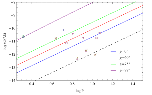
Figure 2: Death-lines for the misaligned magnetar for different values of the inclination angle $\chi$. The value of $\kappa$ is taken to be $0.1$. The dashed line indicates the position of the death-line from IS07. The moment of inertia of the magnetar is taken to be $I=10^{45}\mathrm{g}\mathrm{cm}^{2}$. Crosses and squares indicate the position of soft gamma-ray repeaters and anomalous X-ray pulsars, respectively. Anomalous X-ray pulsars from which the radio emission has been registered are marked with ticks, radio-loud soft gamma-ray repeater is enclosed in circle.

As a next step we investigate the dependence of the magnetar death-line on the inclination angle between the angular momentum of the magnetar and its magnetic moment. By using Eq. (LABEL:Mus_phi) with nonzero $\chi$, we obtain the following expression for the minimum mean free path of the curvature photons

where

$$\tilde{a}=\frac{\kappa}{f(1)}\cos\chi\ ,\quad\tilde{b}=\frac{3}{4}\frac{R_{s}^{1/2}}{R_{c}^{1/2}}\frac{H(1)}{(f(1))^{3/2}}\left(\frac{\Theta(\eta)}{\Theta_{0}H(1)}-1\right)\sin\chi\ ,$$ (9)

while $\xi_{min}$ may be found as a solution of the cubic equation

$$11\tilde{b}\xi_{min}^{3}+8\tilde{a}\xi_{min}^{2}-5\tilde{b}\xi_{min}-2\tilde{b}\xi_{min}=0\ ,$$ (10)

obtained by setting to zero the derivative of the mean free path $l_{f}$. We note that in the derivation of Eq. (10) we have used the fact that $\tilde{b}>0$, so the minimum of the mean free path $l_{f}$ corresponds to the value $\cos\phi=1$. As already mentioned above, at the considered distances from the star surface we are allowed to use the values of the functions $H(\eta)$ and $f(\eta)$ in the limit of large $\eta$, therefore adopting $H(\eta)\approx f(\eta)\approx 1$. The value of $\Theta(\eta)/\Theta_{0}$, on the other hand, is determined after using equation (3) in the small angle approximation. Under these assumptions we have solved Eq. (10) numerically finding the following expression for the death-line of the inclined magnetar:

In Fig.2 we have reported a few death-lines for magnetars having different inclination angles, while keeping the same compactness parameter $\kappa=0.1$. This figure shows that, by increasing the angle $\chi$ between the angular momentum vector of the star and its magnetic moment, the death-line is shifted upwards. Although this effect is even more pronounced than that produced by purely general relativistic effects, its physical relevance for explaining the radio-quietness of magnetars cannot be over-emphasized, since it would imply a implausible strong misalignment in all magnetars that have been observed.

3 Death-line for the rotating and oscillating magnetars

In this section we consider magnetars that are subject to toroidal oscillations, relying on results obtained by Timokhin (2007) and Morozova et al. (2010). In spherical coordinates $(r,\theta,\phi)$ the velocity field of an oscillating neutron star can be written as (Unno et al. 1989)

$$\delta v^{\hat{i}}=\left\{0,\frac{1}{\sin\theta}\partial_{\phi}Y_{lm}(\theta,\phi),-\partial_{\theta}Y_{lm}(\theta,\phi)\right\}\tilde{\eta}(r)e^{-i\omega t}\ ,$$ (12)

where $\tilde{\eta}$ is the radial eigenfunction expressing the amplitude of the oscillation, $\omega$ is the frequency of oscillation and the orthonormal functions $Y_{lm}(\theta,\phi)$ are the eigenfunctions of the Laplacian in spherical coordinates.

The electromagnetic scalar potential in the polar cap region of rotating and oscillating aligned neutron star magnetosphere has been computed by Morozova et al. (2010) and it is given by

This equation differs from the analogous equation (33) by Morozova et al. (2010) in one fundamental respect. Namely, the oscillatory part of the scalar potential is missing the term proportional to $1/r^{2}$ that was reported in Eq. (33) by Morozova et al. (2010), because we have taken the asymptotic value as discussed above.

For any particular mode $(l,m)$, we use the approximation $Y_{lm}(\theta,\phi)\approx A_{lm}(\phi)\theta^{m}$, valid in the limit of small polar angles $\theta$, where the terms $A_{lm}(\phi)$ have real parts given by

$$A_{00} = \frac{1}{\sqrt{4\pi}}\ ,$$ (14)

$$A_{10} = \sqrt{\frac{3}{4\pi}}\ ,$$ (15)

$$A_{11} = -\sqrt{\frac{3}{8\pi}}\cos\phi\ ,$$ (16)

$$A_{20} = \sqrt{\frac{5}{4\pi}}\ ,$$ (17)

$$A_{21} = -3\sqrt{\frac{5}{24\pi}}\cos\phi\ .$$ (18)

In addition, since we do not explore the time evolution of the system, in the calculations that follow we drop the time dependence of the oscillatory term (computed at time $t=0$ as in Morozova et al. (2010)), we then recall the definition $\xi=\theta/\Theta$, and we therefore rewrite Eq. (LABEL:Psi1) as

$$\Psi(\xi,\phi)_{lm} = \frac{B_{0}}{2}\frac{R_{s}^{3}}{R_{c}^{2}}\frac{\kappa}{f(1)}\left(1-\xi^{2}\right)-$$ (19)

$$\tilde{\eta}(R_{s})\frac{B_{0}}{f^{m}(1)}\frac{R_{s}^{\frac{m}{2}+1}}{R_{c}^{\frac{m}{2}}}\xi^{m}A_{lm}(\phi)\ ,$$

where one takes into account the expressions (3) and (4) for the $\Theta$ and $\Theta_{0}$, respectively.

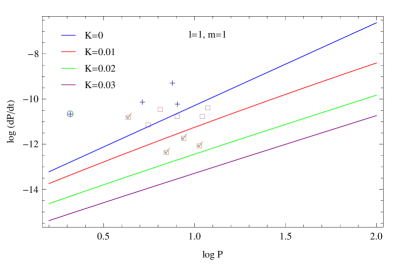
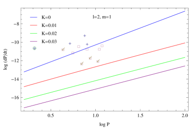
Figure 3: Death-lines for rotating and oscillating magnetars in the $P-\dot{P}$ diagram. The left panel corresponds to the mode $(1,1)$ and values of $K=0\ ,0.01\ ,0.02\ ,0.03$. The right panel corresponds to the mode $(2,1)$ and values of $K=0\ ,0.01\ ,0.02\ ,0.03$. Other parameters are taken to be $R_{s}=10\mathrm{km}$, $M=2M_{\bigodot}$ and $\kappa=0.15$. Crosses and squares indicate the position of soft gamma-ray repeaters and anomalous X-ray pulsars, respectively. Anomalous X-ray pulsars from which the radio emission has been registered are marked with ticks, radio-loud soft gamma-ray repeater is enclosed in circle.

At this point, by repeating the procedure already described in Sec. 2.2 and 2.3, but with the scalar potential in the polar cap region given by Eq. (19), we find the mean free path of the curvature photon in the form

The minima of (LABEL:l_f_oscill) clearly depends on the choice of the mode $(l,m)$ that is considered. For example, for $m\neq 0$, the minimum of $l_{f}$ comes after solving the following quadratic equation

$$8a\xi_{min}^{2}+(2b+3mb)\xi_{min}^{m}=2a\ ,$$ (21)

where

$$a=\frac{B_{0}}{2}\frac{R_{s}^{3}}{R_{c}^{2}}\frac{\kappa}{f(1)}\ ,\qquad b=\tilde{\eta}(R_{s})\frac{B_{0}}{f^{m}(1)}\frac{R_{s}^{\frac{m}{2}+1}}{R_{c}^{\frac{m}{2}}}A_{lm}(\phi)\ .$$ (22)

When $m=1$ and $m=2$ the solution of equation (21) is given by

$$\xi_{min} = \frac{-5b+\sqrt{25b^{2}+64a^{2}}}{16a}\ \ \ \ \ \ \ \ \ \rm{for}\ \ \ \ m=1\ ,and$$ (23)

$$\xi_{min} = \frac{1}{2}\sqrt{\frac{a}{a+b}}\hskip 31.2982pt\ \ \ \ \ \ \ \ \ \ \ \ \ \ \ \ \rm{for}\ \ \ \ m=2\ .$$ (24)

In the absence of oscillations, namely when $b=0$, both cases $m=1$ and $m=2$ give the minimum of $l_{f}$ at the value $\xi_{min}=1/2$, corresponding to the case of pure rotation (Istomin & Sobyanin 2007). After performing an averaging on the azimuthal angle $\phi$, we derive the condition for radio emission on the intensity of the magnetic field, which, for $m\neq 0$, is given by

We then proceed in complete analogy with Sec. 2.2, namely by assuming that the magnetar spins down due to the generation of magnetodipole radiation, so that $B_{0}\simeq 2(P\dot{P}_{-15})^{1/2}10^{12}\mathrm{G}$. In this way the equation of the death-lines for oscillating and rotating neutron stars is

where $\dot{P}_{-15}$ is the period time derivative measured in $10^{-15}\mathrm{s\ s^{-1}}$. The amplitude of the oscillation is now parametrized in terms of the small number $K=\tilde{\eta}(1)/\Omega R$, giving the ratio between the velocity of oscillations and the linear rotational velocity of magnetar. Fig. 3 reports the death-lines for rotating as well as oscillating magnetars for two modes of oscillations and different values of the parameter $K$. In particular, the left panel shows the case $l=1,m=1$, while the right panel shows the case $l=2,m=1$, thus providing the two most relevant physical cases for non-axisymmetric modes. Unlike the effects induced by general relativistic corrections and by the inclination angle $\chi$, which only produce shifting of the death-lines without affecting their slope, changes in the intensity of the oscillation affect both the slope and the shifting of the death-lines. In particular, larger values of $K$ produce smaller slopes (though converging to a constant value) and downward shifting in the $P-\dot{P}$ diagram. On the overall, stronger oscillations of the modes with $m=1$ contribute to radio-loudness of magnetars. This result is in agreement with the work by Morozova et al. (2010), where it was found that that oscillation modes with $m=1$ considerably increase the electromagnetic energy losses from the polar cap region of the neutron star, which may be several times larger than in the case when no oscillations are present.

In a recent paper, Timokhin et al. (2008) invoked stellar oscillations to explain the observed quasi-periodic oscillations in the tail of soft gamma repeater giant flares. Such oscillations lie in the range between 18 Hz and 1800 Hz, and are widely interpreted as shear modes of the solid crust of the neutron stars (Steiner & Watts 2009). Timokhin et al. (2008) showed that the stellar oscillations should be of the order of $1\%$ of the stellar radii, in order to explain the observed phenomenology. It is interesting to note that, when translated in terms of our parameter $K$, these estimates imply $K\sim 0.1$ or higher, while we have shown that noticeable effects on the magnetospheric features of the magnetars are already present for $K\sim 0.01-0.03$.

A complementary information to that of Fig. 3 is provided by Fig. 4, where we have plotted the velocity field for a few modes of stellar oscillations (see also Timokhin et al. (2000)). The electron-positron plasma in the neutron star magnetosphere is expected to be continuously generated in the polar cap region, where magnetic field lines are open and the plasma may freely escape from the surface of the star to infinity. When the star rotates, the linear velocity of the stellar surface motion is of course proportional to the distance from the axis of rotation to the considered point. Therefore, in the polar cap region this velocity is proportional to the polar angle. When we limit our attention to the polar cap region, namely by looking at the top of each sphere reported in Fig. 4, we see that the velocity distribution for the oscillatory modes with $m=0$ has the same form as for the case of pure rotation. For the modes $m=1$, on the other hand, the velocity of oscillations remains almost constant across the polar cap region. This further indicates that the modes with $m=1$ have greater impact on the magnetosphere processes and, therefore, merit more attention.

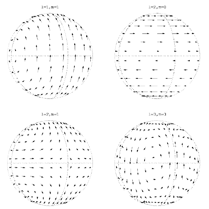
Figure 4: Velocity distribution for a few different modes of stellar oscillations.

4 Conclusions

It was not until 2006 that the first detection of a radio magnetar was reported. To date, only two radio magnetars have been confirmed, namely XTE J1810 —197 and 1E 1547.0-5408 and it remains unclear what is the physical mechanism preventing the radio-loudness of these sources.

In this work, by using the general relativistic expression for the accelerating electromagnetic scalar potential in the vicinity of the polar cap, we have performed a detailed analysis of the position of the death-line in the $P-\dot{P}$ diagram. Our results can be summarized as follows:

• When the compactness of the neutron star is increased, the death line shifts upwards in the $P-\dot{P}$ diagram, pushing the magnetar in the radio-quiet region. This is a purely general relativistic effect.

• When the inclination angle $\chi$ between the angular momentum vector of the neutron star and its magnetic moment is increased, the death-line shifts upwards in the $P-\dot{P}$ diagram, pushing the magnetar in the radioquiet region.

• On the contrary, when oscillations of the magnetar are taken into account, the radio emission from the magnetosphere is generally favored. In fact, the major effect of oscillations is to amplify the scalar potential in the polar cap region of the magnetar magnetosphere. As a result, the energy of primary particles that are pulled out and accelerated in the vicinity of the stellar surface is enhanced, and the probability of effective electron-positron plasma generation is increased. The largest effect is expected for oscillation modes with $m=1$, whose velocity field is almost uniform in the polar cap region.

It is worth stressing that, according to our explanation, there is not a unique death line which is valid for the entire class of magnetars. On the contrary, each source has its own death line that is determined by individual physical conditions. This also implies that a source in the $P-\dot{P}$ diagram may be radio-quiet while another source, located below the first one, is radio-loud, just because their death-lines are different. While providing an effective explanation of magnetar radio-quieteness in terms of the stellar compactness and of the misalingment between angular momentum and magnetic moment, our results may also indicate that the unusual radio emission observed from some magnetars may be related to the generation of oscillations in the magnetar crust. This hypothesis is sustained by the registration of preceding bursts from these magnetars. According to this interpretation, one may expect that after the magnetar burst, which produces mechanical oscillations of the stellar crust, the conditions for radio emission within the magnetospehere are satisfied. However, because of the inevitable damping of the oscillations, after a damping time the magnetar will turn back to the radioquiet region in the $P-\dot{P}$ diagram (the deathline will shift back upwards). This is qualitatively in agreement with observations showing that in radio-loud magnetars the radio emission reveals strong fluctuations in time. This is particularly true for the candidate radio-magnetars which may be located at the border between radio-loud and radio-quiet regions (see Malofeev et al. (2007), Malofeev et al. (2010)). Future more accurate observations are likely to verify or refute our interpretation by testing if there is a close connection between the burst activity of magnetars and the generation of the radio emission in the magnetar magnetosphere.

References

- Abdikamalov et al. (2009) Abdikamalov E. B., Ahmedov B. J., Miller J. C., 2009, Mon. Not. R. Astron. Soc., 395, 443
- Ahmedov & Morozova (2009) Ahmedov B. J., Morozova V. S., 2009, Astrophys. Space. Sci., 319, 115
- Arons & Scharlemann (1979) Arons J., Scharlemann E. T., 1979, Astrophys. J., 231, 854
- Barat et al. (1983) Barat C., Hayles R. I., Hurley K., Niel M., Vedrenne G., Desai U., Kurt V. G., Zenchenko V. M., Estulin I. V., 1983, Astron. Astrophys., 126, 400
- Beskin et al. (1993) Beskin V. S., Gurevich A. V., Istomin Ya. N., 1993, Physics of the Pulsar Magnetosphere. Cambridge University Press, Cambridge
- Beskin (2010) Beskin V. S., 2010, MHD Flows in Compact Astrophysical Objects: Accretion, Winds and Jets. Springer-Verlag, Berlin
- Camilo et al. (2006) Camilo F., Ransom S. M., Halpern J. P., Reynolds J., Helfand D. J., Zimmerman N., Sarkissian J., 2006, Nature, 442, 892
- Camilo et al. (2007) Camilo F., Ransom S. M., Halpern J. P., Reynolds J., 2007, Astrophys. J., 666, L93
- Chen & Ruderman (1993) Chen K., Ruderman M. A., 1993, Astrophys. J., 402, 264
- Colaiuda & Kokkotas (2011) Colaiuda A., Kokkotas K. D., 2011, Mon. Not. R. Astron. Soc., 414, 3014
- Duncan (1998) Duncan R. C., 1998, Astrophys. J. Lett., 498, L45+
- Duncan & Thompson (1992) Duncan R. C., Thompson C., 1992, Astrophys. J. Lett., 392, L9
- Eichler & Shaisultanov (2010) Eichler D., Shaisultanov R., 2010, Astrophys. J. Lett., 715, L142
- Glampedakis et al. (2007) Glampedakis K., Samuelsson L., Andersson N., 2007, Astrophys. Space Sci., 308, 607
- van Hoven & Levin (2011) van Hoven M., Levin Yu., 2011, Mon. Not. R. Astron. Soc., 410, 1036
- Hurley (2009) Hurley K., 2009, in Becker W., ed., Neutron Stars and Pulsars, Springer-Verlag, Berlin, p.575
- Israel et al. (2005) Israel G. L., Belloni T., Stella L., Rephaeli Y., Gruber D. E., Casella P., Dall’Osso S., Rea N., Persic M., Rothschild R. E., 2005, Astrophys. J. Lett., 628, L53
- Istomin & Sobyanin (2007) Istomin Y. N., Sobyanin D. N., 2007, Astronomy Letters, 33, 660
- Kantor & Tsygan (2004) Kantor E. M., Tsygan A. I., 2004, Astronomy Reports, 48, 1029
- Kramer (2008) Kramer M., 2008, in Strassmeier K. G., Kosovichev A. G., Beckman J. E., eds, Cosmic Magnetic Fields: From Planets, to Stars and Galaxies, Proceedings IAU Symposium No. 259, p. 485
- Levin (2007) Levin Yu., 2007, Mon. Not. R. Astron. Soc., 377, 159
- Levin et al. (2010) Levin L., Bailes M., Bates S., Bhat N. D. R., Burgay M., Burke-Spolaor S., D’Amico N., Johnston S., Keith M., Kramer M., Milia S., Possenti A., Rea N., Stappers B., van Straten W., 2010, Astrophys. J. Lett., 721, L33
- Malheiro et al. (2011) Malheiro M., Rueda J. A., Ruffini R., 2011, eprint arXiv:1102.0653
- Malofeev et al. (2007) Malofeev V. M., Malov O. I., Teplykh D. A., 2007, Astrophys. Space. Sci., 308, 211
- Malofeev et al. (2010) Malofeev V. M., Teplykh D. A., Malov O. I., 2010, Astronomy Reports, 54, 995
- Manchester et al. (2005) Manchester R. N., Hobbs G. B., Teoh A., Hobbs M., 2005, Astron. J., 129, 1993
- McDermott et al. (1988) McDermott P. N., van Horn H. M., Hansen C. J., 1988, Astrophys. J., 325, 725
- Morozova et al. (2010) Morozova V. S., Ahmedov B. J., Zanotti O., 2010, Mon. Not. R. Astron. Soc., 408, 490
- Muslimov & Harding (1997) Muslimov A., Harding A. K., 1997, Astrophys. J., 485, 735
- Muslimov & Tsygan (1992) Muslimov A. G., Tsygan A. I., 1992, Mon. Not. R. Astron. Soc., 255, 61
- Rudak & Ritter (1994) Rudak B., Ritter H., 1994, Mon. Not. R. Astron. Soc., 267, 513
- Ruderman & Sutherland (1975) Ruderman M. A., Sutherland P. G., 1975, Astrophys. J., 196, 51
- Schumaker & Thorne (1983) Schumaker B. L., Thorne K. S., 1983, Mon. Not. R. Astron. Soc., 203, 457
- Steiner & Watts (2009) Steiner A. W., Watts A. L., 2009, Phys. Rev. Lett., 103, 181101
- Strohmayer & Watts (2006) Strohmayer T. E., Watts A. L., 2006, Astrophys. J., 653, 593
- Terasawa et al. (2005) Terasawa T., Tanaka Y. T., Takei Y., Kawai N., Yoshida A., Nomoto K., Yoshikawa I., Saito Y., Kasaba Y., Takashima T., Mukai T., Noda H., Murakami T., Watanabe K., Muraki Y., Yokoyama T., Hoshino M., 2005, Nature, 434, 1110
- Timokhin et al. (2000) Timokhin A. N., Bisnovatyi-Kogan G. S., Spruit H. C., 2000, Mon. Not. R. Astron. Soc., 316, 734
- Timokhin (2007) Timokhin A. N., 2007, Astropys. Space Sci., 308, 345
- Timokhin et al. (2008) Timokhin A. N., Eichler D., Lyubarsky Yu., 2008, Astrophys. J., 680, 1398
- Unno et al. (1989) Unno W., Osaki Y., Ando H., Saio H., Shibahashi H., 1989, Nonradial Oscillations of Stars. Univ. Tokyo Press, Tokyo
- Woods & Thompson (2006) Woods P. M., Thompson C., 2006, in Lewin W., van der Klis M., eds, Compact Stellat X-ray Sources, Cambridge University Press, New York, p.547
- Zhang et al. (2000) Zhang B., Harding A. K., Muslimov A. G., 2000, Astrophys. J., 531, L135