Fluctuation Probes of Early-Time Correlations in Nuclear Collisions

Abstract

Correlation measurements imply that anisotropic flow in nuclear collisions includes a novel triangular component along with the more familiar elliptic-flow contribution. Triangular flow has been attributed to event-wise fluctuations in the initial shape of the collision volume. We ask two questions: 1) How do these shape fluctuations impact other event-by-event observables? 2) Can we disentangle fundamental information on the early time fluctuations from the complex flow that results? We study correlation and fluctuation observables in a framework in which flux tubes in an early Glasma stage later produce hydrodynamic flow. Calculated multiplicity and transverse momentum fluctuations are in excellent agreement with data from 62.4 GeV Au+Au up to 2.76 TeV Pb+Pb.

I Introduction

Measurements of two particle correlations in nuclear collisions exhibit a complex pattern of ridges, bumps, and valleys as functions of relative pseudorapidity $\Delta\eta=\eta_{1}-\eta_{2}$ and azimuthal angle $\Delta\phi=\phi_{1}-\phi_{2}$ Putschke (2007); Abelev (2009); Nattrass (2009); Daugherity (2008); De Silva (2009); Adams et al. (2006); Adamova et al. (2008); Alver et al. (2008, 2009). In a recent advance, Alver and Roland showed that much of the $\Delta\phi$ dependence of these correlations can be described in terms of anisotropic flow Alver and Roland (2010). Their key realization was that a novel triangular flow contribution $\sim v_{3}\cos 3\Delta\phi$ is needed to describe the data. Such contributions have been attributed to fluctuations of the geometric shape of the collision volume from event to event Takahashi et al. (2009); Alver and Roland (2010); Alver et al. (2010); Sorensen (2010); Sorensen et al. (2011); Luzum (2010); Petersen et al. (2010); Qin et al. (2010); Petersen and Bleicher (2010); Teaney and Yan (2010); Schenke et al. (2011); Qiu and Heinz (2011). A unique shape is determined in the first instants of each collision event as the nuclei crash through one another.

Interestingly, fluctuations have been of measured in nuclear collisions for many years, but for different reasons. Event-by-event fluctuations of the multiplicity, mean transverse momentum, and net charge are viewed as probes of the QCD phase transition, although signature behavior has yet to be seen Westfall (2008); Koch (2008); Aggarwal et al. (2010). Such observations are explained by the variation of density, geometry, thermalization, and flow; see, e.g., Gavin (2004, 2004); Voloshin (2006); Mrowczynski et al. (2004); Broniowski et al. (2009).

In this paper we explore the common influence that the early-time dynamics of the system has on correlations, flow, and fluctuations. We begin by asking how geometric fluctuations impact other event-by-event observables. In Sec. II, we recall the relationship between correlations and anisotropic flow. Next, we discuss the relationship between fluctuations and correlations in Sec. III. We exploit integral relationships obtained in Ref. Pruneau et al. (2002) to marry the dynamical language of flow and correlations to the statistical formulation of fluctuation observables. This yields model independent properties of experimental observables. In particular, we find that geometric shape fluctuations alone cannot explain measured multiplicity and transverse momentum fluctuations.

We next ask what fluctuation and correlation measurements can reveal about the early-time dynamics of the collision system. The first evidence that correlations originate at early times in the collision is the long rapidity range of the ridge Dumitru et al. (2008); Gavin et al. (2009). Correlations show a ridge-like peak near $\Delta\phi=0$. This ridge extends over a broad range in $\Delta\eta$, as do away-side features centered near $\Delta\phi\sim\pi$ Alver et al. (2008). Causality dictates that correlations over several rapidity units must originate at the earliest stages of the collision Dumitru et al. (2008); Gavin et al. (2009). With that in mind, we described the ridge as a consequence of particle production in an early Glasma stage followed by transverse flow in Refs.  Dumitru et al. (2008); Gavin et al. (2009); Moschelli and Gavin (2010); Dusling et al. (2009). Our description is part of a broader family of models in which particles are initially correlated at the point of production Voloshin (2006); Pruneau et al. (2008); Lindenbaum and Longacre (2007); Peitzmann (2009); Takahashi et al. (2009); Andrade et al. (2010); Werner et al. (2010); Sharma et al. (2011).

Identifying the impact of anisotropic flow on these correlations adds considerable credence to this observation Sorensen et al. (2011). Anisotropic flow is well understood as an early time effect, since it is generated in part by the geometric configuration of participant nucleons in the colliding nuclei; see, e.g., Voloshin et al. (2008); Sorensen (2009). Correspondingly, the measured $v_{2}$ coefficients vary little with rapidity.

To illustrate how correlations, flow, and fluctuations result from the early-time dynamics, we apply the general framework of Refs. Gavin et al. (2009); Moschelli and Gavin (2010) in Sec. IV. We obtain expressions for the correlation function and its Fourier coefficients, (23), (24), and (25). This provides a unifying framework for understanding hydrodynamic $v_{n}$ studies together with earlier work on the ridge. We also derive expressions for transverse momentum fluctuations, (26) and (27).

In Sec. V, we use fluctuation measurements to extract information on the particle production mechanism. We focus on the Color Glass Condensate formulation in Ref. Dumitru et al. (2008); Gavin et al. (2009); Dusling et al. (2009); Moschelli and Gavin (2010), and argue that dynamic multiplicity fluctuations $\cal R$ can provide information on particle production that is independent of flow. Transverse momentum fluctuations $\langle\delta p_{t1}\delta p_{t2}\rangle$ provide similar information, although the results are somewhat sensitive to radial flow (but not the $v_{n}$). Constraining the flow contribution by calculating $\langle p_{t}\rangle$ and $v_{2}$, we compute the fluctuations for $\cal R$ and $\langle\delta p_{t1}\delta p_{t2}\rangle$. We find that the same model that described the energy, target-mass, and $p_{t}$ dependence of the ridge also describes transverse momentum fluctuations measured at the Brookhaven Relativistic Heavy Ion Collider, RHIC, and the CERN Large Hadron Collider LHC.

II Correlations and Flow

Correlation measurements commonly center on the pair distribution

$$\rho_{2}(\mathbf{p}_{1},\mathbf{p}_{2})={{dN}\over{d\eta_{1}d^{2}p_{t1}d\eta_{2}d^{2}p_{t2}}},$$ (1)

where $\eta_{i}$ is pseudorapidity and $p_{ti}=|\mathbf{p}_{ti}|$ is transverse momentum of particles $i=1,2$. In the absence of correlations, $\rho_{2}(\mathbf{p}_{1},\mathbf{p}_{2})\rightarrow\rho_{1}(\mathbf{p}_{1})\rho_{1}(\mathbf{p}_{2})$, where the single particle distribution is $\rho_{1}(\mathbf{p})=dN/d\eta d^{2}p_{t}$. Experiments typically report ratios of $\rho_{2}$ to either $\rho_{1}\rho_{1}$ or mixed event pairs integrated over ranges of $p_{t}$. To keep the notation simple, we will not make the $\eta$ dependence explicit unless needed.

To illustrate the connection between flow and correlations, recall for the moment the traditional picture of flow in which event-by-event fluctuations are neglected. It has long been known that collisions at non-zero impact parameter $b$ produce anisotropic flow Voloshin et al. (2008); Sorensen (2009). Anisotropy derives from the change in the shape of the collision volume with respect to the reaction plane, i.e., the plane spanned by $\mathbf{b}$ and the beam direction. The distribution with respect to this plane is

$$\rho_{1}(\mathbf{p}_{t};\psi_{{}_{RP}})=\overline{\rho}_{1}\{1+2\sum_{n=1}^{\infty}v_{n}(p_{t})\cos[n(\phi-\psi_{{}_{RP}})]\},$$ (2)

where the coefficients depend only on the magnitude $p_{t}=|\mathbf{p}_{t}|$ and $\eta$. An experimental analysis that does not identify the reaction plane measures the distribution $(2\pi)^{-1}\int\rho_{1}(\mathbf{p}_{t};\psi_{{}_{RP}})d\psi_{{}_{RP}}=\overline{\rho}_{1}$, where the “bar” denotes average over $\phi$. The second equality follows because $\rho_{1}$ is a function of $\phi-\psi_{{}_{RP}}$.

Anisotropic flow introduces correlations because pairs from the same collision event have the same reaction plane. The reaction plane averaged pair distribution can only be a function of the relative angle $\Delta\phi$, so that

$${\rho}_{2}=\overline{\rho}_{2}\{1+2\sum_{n=1}^{\infty}a_{n}(p_{1},p_{2})\cos(n\Delta\phi)\}.$$ (3)

If geometry is the only source of correlations then ${\rho}_{2}(\mathbf{p}_{t1},\mathbf{p}_{t2})$ is the product $\rho_{1}(\mathbf{p}_{t1};\psi_{{}_{RP}})\rho_{1}(\mathbf{p}_{t2};\psi_{{}_{RP}})$ averaged over $\psi_{{}_{RP}}$. In that case the Fourier coefficients of (2) and (3) are related. For $n=0$ we find

$$\overline{\rho}_{2}(p_{1},p_{2})\rightarrow\overline{\rho}_{1}(p_{1})\overline{\rho}_{1}(p_{2}).\,\,\,\,\,\,\,\,\,\,\,\,\,\,\,\,{\rm uncorrelated}$$ (4)

while for $n\geq 2$

$$a_{n}(p_{1},p_{2})\rightarrow{v_{n}(p_{1})v_{n}(p_{2})};\,\,\,\,\,\,\,\,\,\,\,\,{\rm uncorrelated}$$ (5)

these results hold only when fluctuations may be neglected. Momentum conservation contributes to $a_{1}$, modifying the $v_{1}(p_{1})v_{1}(p_{2})$ term, as discussed by Borghini and others Borghini et al. (2002); Borghini (2003, 2007, 2007); Chajecki and Lisa (2008).

Fluctuations introduce further anisotropy because the shape of the collision volume is different in each collision event. In collisions of identical nuclei, the event-averaged interaction volume is symmetric in $\phi$ and fixed by $b$ and $\Psi_{{}_{RP}}$. If all events of a given $b$ had the same interaction volume, we then would expect only even $n$ to contribute to (2). Shape fluctuations cause the flow parameters $v_{n}$ to vary from event to event and allow odd $n$ to contribute. The average pair distribution has the same form as (3), but with coefficients

$$a_{n}(p_{1},p_{2})=\langle{v_{n}(p_{1})v_{n}(p_{2})}\rangle,$$ (6)

where the brackets denote average over events (including all event shapes) Teaney and Yan (2010). The measured azimuthal dependence of two particle correlations are reasonably described by (3) with $n=1,2$ and $3$. We emphasize that fluctuations in shape alone cannot alter $\overline{\rho}_{2}$ – this requires further dynamical fluctuations which we discuss in the next sections.

We remark in passing that one often discusses the shape fluctuations in terms of a geometric eccentricity $\epsilon_{n}$. If one assumes that the relation between $\epsilon_{n}$ and the resulting anisotropy of the fluid flow $v_{n}$ is approximately deterministic, then fluctuations of the ratio $v_{n}(p_{1})/\epsilon_{n}$ are negligible. In that case $\langle{v_{n}(p_{1})v_{n}(p_{2})}\rangle\approx(v_{n}(p_{1})/\epsilon_{n})(v_{n}(p_{2})/\epsilon_{n})\langle\epsilon_{n}^{2}\rangle$. This factorization conjecture seems plausible, but currently requires further theoretical investigation Luzum (2011).

III Fluctuations

Fluctuation measurements study the variation of bulk quantities, such as multiplicity or average transverse momentum, over an ensemble of events Gazdzicki and Mrowczynski (1992); Mrowczynski (1998); Westfall (2008). Suppose that fluctuations of multiplicity $N$ result in a variance $\sigma_{{}_{N}}^{2}=\langle N^{2}\rangle-\langle N\rangle^{2}$. Uncorrelated particles would be described by Poisson statistics, for which $\sigma_{{}_{N}}^{2}\rightarrow\sigma_{\rm stat}^{2}=\langle N\rangle$. Correlations give rise to a difference $\sigma_{{}_{N}}^{2}-\sigma_{\rm stat}^{2}$, which we characterize by the dynamic variance

$${\cal R}={{\langle N^{2}\rangle-\langle N\rangle^{2}-\langle N\rangle}\over{\langle N\rangle^{2}}},$$ (7)

as discussed in Pruneau et al. (2002). Similarly, many describe the dynamic fluctuations of transverse momentum using the covariance

$$\langle\delta p_{t1}\delta p_{t2}\rangle={{\langle\sum_{i\neq j}\delta p_{ti}\delta p_{tj}\rangle}\over{\langle N(N-1)\rangle}},$$ (8)

where $\delta p_{ti}=p_{ti}-\langle p_{t}\rangle$ and the average transverse momentum is $\langle p_{t}\rangle=\langle P_{t}\rangle/\langle N\rangle$ for $P_{t}=\sum_{i}p_{ti}$ the total momentum in an event Voloshin et al. (1999); Voloshin (2001); Adamova et al. (2003); Adams et al. (2005). This quantity vanishes when particles $i$ and $j$ are uncorrelated. Note that one can write $\langle\delta p_{t1}\delta p_{t2}\rangle$ in terms of the variance $\sigma_{P_{t}}^{2}=\langle(P_{t}-N\langle p_{t}\rangle)^{2}\rangle$. In the absence of correlations, that variance is $\sigma_{P_{t}\,{\rm stat}}^{2}=\langle N\rangle(\langle p_{t}^{2}\rangle-\langle p_{t}\rangle^{2})$. One can show that $\langle\delta p_{t1}\delta p_{t2}\rangle$ is the difference $\sigma_{P_{t}}^{2}-\sigma_{P_{t}\,{\rm stat}}^{2}$ divided by the average number of pairs $\langle N(N-1)\rangle$.

To see the connection between fluctuation and correlation measurements, observe that the integral of the pair distribution $\rho_{2}$ gives the average number of pairs $\langle N(N-1)\rangle$. We then write (7) as

$${\cal R}={{1}\over{\langle N\rangle^{2}}}\int r(\mathbf{p}_{1},\mathbf{p}_{2})d\mathbf{p}_{1}d\mathbf{p}_{2},$$ (9)

where we define

$$r(\mathbf{p}_{1},\mathbf{p}_{2})={\rho}_{2}(\mathbf{p}_{1},\mathbf{p}_{2})-{\rho}_{1}(\mathbf{p}_{1}){\rho}_{1}(\mathbf{p}_{2}).$$ (10)

Similarly, we can write (8) in terms of the correlation function (10) as

$$\langle\delta p_{t1}\delta p_{t2}\rangle=\int\!d\mathbf{p}_{1}d\mathbf{p}_{2}\,{{r(\mathbf{p}_{1},\mathbf{p}_{2})}\over{\langle N(N-1)\rangle}}\delta p_{t1}\delta p_{t2}.$$ (11)

We stress that the densities $\rho_{1}$ and $\rho_{2}$ are event-averaged quantities.

Fluctuation measurements probe the overall strength of correlations in a manner that is independent of the anisotropic flow. To see this, we combine (3) with (10) to find that the $\cos n\Delta\phi$ contributions vanish on integration over $0\leq\Delta\phi\leq 2\pi$. We obtain

$${\cal R}={{1}\over{\langle N\rangle^{2}}}\int\overline{r}(p_{t1},p_{t2})d\mathbf{p}_{1}d\mathbf{p}_{2},$$ (12)

which depends only on the $\phi$ averaged function

$$\overline{r}(p_{t1},{p}_{t2})=\overline{\rho}_{2}(p_{t1},p_{t2})-\overline{\rho}_{1}(p_{t1})\overline{\rho}_{1}(p_{t2}).$$ (13)

It is easy to understand why ${\cal R}$ is not sensitive anisotropy – $N$ simply counts particles irrespective of where they are flowing. Similarly, the

$$\langle\delta p_{t1}\delta p_{t2}\rangle=\int\!d\mathbf{p}_{1}d\mathbf{p}_{2}\,{{\overline{r}(p_{t1},p_{t2})}\over{\langle N(N-1)\rangle}}\delta p_{t1}\delta p_{t2},$$ (14)

Here too the $\cos n\Delta\phi$ contributions to (3) vanish on integration. These fluctuations are independent of $\phi$ because our definition of $p_{ti}$ disregards direction.

Equations (12) and (13) have two striking implications when combined with flow results from the previous section. First, if the variation of the initial geometric shape of the collision volume is the only source of fluctuations then (4) implies that ${\cal R}$ and $\langle\delta p_{t1}\delta p_{t2}\rangle$ must both vanish. Experiments have measured these quantities and they are both nonzero, as shown in Sec. V. Second, the amplitudes $\overline{r}$ and $\overline{\rho}_{2}$ determine the overall magnitude of correlations, as we see from (3). Anisotropic flow and momentum conservation determine the coefficients (6) and, therefore, the relative height of the near-side “ridge” at $\Delta\phi=0$ and away-side features near $\Delta\phi=\pi$. However, interpretation of the evolution of the ridge height with beam energy or centrality requires an understanding of $\overline{r}$ or $\cal R$.

IV Source of Fluctuations

Nuclear collisions vary sharply from event to event due to differences in the number and configuration of the nucleons struck in the initial impact. Each strike adds to a transient color field that lasts a proper time of roughly $\tau_{0}\sim 1$ fm. This field comprises an array of flux tubes connecting the fragments of the highly Lorentz-contracted nuclei along the beam direction. The number of participants determines the color charge and thus the overall strength of the fields. The flux tubes fragment after $\tau_{0}$, driving soft particle production. We emphasize that flux tubes arise naturally in QCD and have long been the core of phenomenological models such as PYTHIA. In the next section we will focus on the Color Glass Condensate description, which incorporates these features in the high density environment produced by nuclear collisions and allows for systematic computations. For now, we keep the discussion more general.

We assume that the number and geometrical distribution of flux tubes is the most important source of fluctuations. Their fragmentation leads to density correlations described by

$$c(\mathbf{x}_{1},\mathbf{x}_{2})=n_{2}(\mathbf{x}_{1},\mathbf{x}_{2})-n_{1}(\mathbf{x}_{1})n_{1}(\mathbf{x}_{2}),$$ (15)

where $n_{1}$ and $n_{2}$ are the single and pair densities. In the absence of correlations, $n_{2}(\mathbf{x}_{1},\mathbf{x}_{2})\rightarrow n_{1}(\mathbf{x}_{1})n_{1}(\mathbf{x}_{2})$ so that $c$ vanishes. The integral of $n_{2}$ over position gives the number of pairs averaged over events, $\langle N(N-1)\rangle$, so that the integral of $c$ is ${\cal{R}}\langle N\rangle^{2}$, with $\cal R$ given by (7). We now take the flux tubes to be longitudinally boost invariant, so that the correlation function only depends on transverse coordinates $\mathbf{r}_{t}=\mathbf{r}_{1,\,t}-\mathbf{r}_{2,\,t}$ as well as the average $\mathbf{R}_{t}=(\mathbf{r}_{1,\,t}+\mathbf{r}_{2,\,t})/2$. We further assume particles from the same flux tube are primordially correlated and that correlations with the reaction plane arise due to the distribution of tubes. Since the transverse size of the flux tube is small, the primordial correlations reflect common spatial origins. We then write

$$c(\mathbf{x}_{1},\mathbf{x}_{2})={\cal R}{\langle N\rangle}^{2}\,\delta(\mathbf{r}_{t})\rho_{{}_{FT}}(\mathbf{R}_{t}).$$ (16)

Here, $\rho_{{}_{FT}}(\mathbf{R}_{t})$ is the probability distribution for finding a flux tube at a transverse position $\mathbf{R}_{t}$ in the collision volume. This function describes the distribution of shape fluctuations discussed earlier. Following Ref. Gavin et al. (2009); Moschelli and Gavin (2010), we take $\rho_{{}_{FT}}$ to roughly follow the participant distribution of the colliding nuclei

$$\rho_{{}_{FT}}(\mathbf{R}_{t})\approx\frac{2}{\pi R^{2}_{A}}\left(1-\frac{R_{t}^{2}}{R_{A}^{2}}\right)$$ (17)

for $R_{t}\leq R_{A}$, and zero otherwise.

We now discuss the impact of these long range correlations on the final-state distributions. Comoving partons locally thermalize as the flux tubes fragment. Pressure builds and transverse expansion begins. In this process, partons from a flux tube at an initial space-time point $(t,\mathbf{x})$ will eventually acquire a final flow four velocity $u^{\mu}$. In a blast wave model $u^{\mu}$ is taken to have a Hubble-like correlation, while hydrodynamic calculations provide a more realistic $u^{\mu}$. In either case, the Cooper-Frye single particle distribution is

$$\rho_{1}(\mathbf{p})=\int f(\mathbf{x},\mathbf{p})\,d\Gamma,$$ (18)

where $f$ is one-body phase space distribution function and $d\Gamma=p^{\mu}d\sigma_{\mu}$ is the element of flux through the four dimensional freeze out surface. In local equilibrium the distribution has the Boltzmann form $f(\mathbf{x},\mathbf{p})={(2\pi)^{-3}}\exp\{-p^{\mu}u_{\mu}/T\}$. The temperature $T$ and fluid four-velocity $u_{\mu}$ are generally fixed by hydrodynamics, which enforces the local conservation laws. In keeping with the boost-invariant distribution (16), we assume that freeze out occurs at a proper time $\tau_{F}$, so that $p^{\mu}d\sigma_{\mu}=\tau_{F}m_{t}\cosh(y-\eta)d\eta d^{2}r_{t}$, where $\eta=(1/2)\ln((t+z)/(t-z))$ is the spatial rapidity.

The pair distribution has an analogous Cooper-Frye form

$$\rho_{2}(\mathbf{p}_{1},\mathbf{p}_{2})=\int f_{2}(\mathbf{x}_{1},\mathbf{p}_{1},\mathbf{x}_{2},\mathbf{p}_{2})d\Gamma_{1}d\Gamma_{2},$$ (19)

where $f_{2}$ is the two-particle Boltzmann distribution function. In local thermal equilibrium the two particle distribution is

$$f_{2}=n_{2}(\mathbf{x_{1}},\mathbf{x_{2}}){{f(\mathbf{x_{1}},\mathbf{p_{1}})}\over{n(\mathbf{x}_{1})}}{{f(\mathbf{x_{2}},\mathbf{p_{2}})}\over{n(\mathbf{x}_{2})}},$$ (20)

where $n_{1}$ and $n_{2}$ are the single-particle and pair densities discussed earlier, with $n(\mathbf{x})=\int f(\mathbf{x},\mathbf{p})d^{3}p$. This expression satisfies a generalization of the Boltzmann transport equation for $f_{2}$; the factors of $f$ cause the generalized collision terms to vanish just as they do in the one body equation. We omit momentum and energy conservation terms that do not contribute to $\cal{R}$ and $\langle\delta p_{t1}\delta p_{t2}\rangle$.

We understand (20) as follows. In local equilibrium we can divide the system into fluid cells, each of which is in equilibrium at the local temperature $T(\mathbf{x})$ and mean velocity $u^{\mu}(\mathbf{x})$. The momentum distribution in each cell must therefore be $f(\mathbf{x},\mathbf{p})$. The local equilibrium phase space distribution (20) is correlated if there are density correlations between cells or autocorrelations. These correlations are described by the pair density $n_{2}(\mathbf{x_{1}},\mathbf{x_{2}})$. The integral $n_{2}$ over both positions gives the number of pairs averaged over events $\langle N(N-1)\rangle$. In the absence of correlations, $n_{2}(\mathbf{x}_{1},\mathbf{x}_{2})\rightarrow n_{1}(\mathbf{x}_{1})n_{1}(\mathbf{x}_{2})$.

In order to study the angular distribution of fluctuations, we use (18), (19), (20), and (15) to write (10) as

$$r(\mathbf{p}_{1},\mathbf{p}_{2})=\!\!\int c(\mathbf{x}_{1},\mathbf{x}_{2})f(\mathbf{x}_{1},\mathbf{p}_{1})f(\mathbf{x}_{2},\mathbf{p}_{2})d\Gamma_{1}d\Gamma_{2}.$$ (21)

We consider the angular correlation function

$$\Delta\rho=\!\!\int r\,\delta(\Delta\phi-\phi_{1}+\phi_{2})\delta(\Delta\eta-\eta_{1}+\eta_{2})d\mathbf{p}_{1}d\mathbf{p}_{2},$$ (22)

where $r(\mathbf{p}_{1},\mathbf{p}_{2})$ is given by (10). This function probes the $(\Delta\eta,\Delta\phi)$ correlations of particles in the full range of $|\mathbf{p}_{t}|$. Such correlations are dominated by the more abundant low $p_{t}$ particles.

We follow Ref. Gavin et al. (2009); Moschelli and Gavin (2010) and identify $c(\mathbf{x}_{1},\mathbf{x}_{2})$ with (16), a form that describes the system at its formation. This identification omits the effects of diffusion described in Ref. Gavin and Abdel-Aziz (2006). This omission is reasonable only as long as correlations are dominated by pairs separated by $|\eta_{1}-\eta_{2}|>1$.

To clarify the contributions of fluctuations and anisotropic flow to correlations, we expand (22) as a Fourier series. Equation (9) implies that the integral of $\Delta\rho$ over $\Delta\phi$ in a rapidity range gives $\langle N\rangle^{2}{\cal{R}}$. We therefore write

$${{\Delta\rho}\over{\langle N\rangle^{2}}}={{{\cal R}}\over{2\pi}}\{1+2\sum_{n=1}^{\infty}A_{n}\cos(n\Delta\phi)\}.$$ (23)

Next, we compute the Fourier coefficients using (21) together with the correlation function (15 – 17). We find

$$A_{n}=\int d^{2}r_{t}\rho_{{}_{FT}}(\mathbf{r}_{t})[v_{n}(\mathbf{r}_{t})]^{2}$$ (24)

where we define the local flow coefficient

$$v_{n}(\mathbf{r}_{t})=\int\!d\mathbf{p}\;{{f(\mathbf{r}_{t},\mathbf{p})}\over{n(\mathbf{r}_{t1})}}\cos{n\phi}.$$ (25)

Identifying the average over the probability distribution $\rho_{{}_{FT}}$ as the event average, we see that (24) has the form $A_{n}=\langle v_{n}^{2}\rangle$ in (6); see Sec. III. An important caveat is that momentum conservation corrections omitted here will modify the low orders, particularly $A_{1}$ Borghini et al. (2002); Borghini (2003, 2007, 2007); Chajecki and Lisa (2008). We will treat these corrections and present a detailed computation of flow parameters and flow fluctuations elsewhere.

We now compute $\langle\delta p_{t1}\delta p_{t2}\rangle$, combining (21) with (15 – 17) as before to evaluate (11). To simplify the denominator in (11), we note that (7) implies that $\langle N(N-1)\rangle=\langle N\rangle^{2}(1+{\cal R})$. We then obtain

$$\langle\delta p_{t1}\delta p_{t2}\rangle={{{\cal R}}\over{1+{\cal R}}}\int d^{2}r_{t}\rho_{{}_{FT}}(\mathbf{r}_{t})[g(\mathbf{r}_{t})]^{2},$$ (26)

where the local momentum excess is

$$g(\mathbf{r}_{t})=\int\!d\mathbf{p}\;{{f(\mathbf{r}_{t},\mathbf{p})}\over{n(\mathbf{r}_{t})}}\left(p_{t}-\langle p_{t}\rangle\right).$$ (27)

In contrast to the flow coefficients (24), we see that $\langle\delta p_{t1}\delta p_{t2}\rangle$ is proportional to $\cal R$. However, both flow and fluctuation quantities depend on $\rho_{{}_{FT}}$ in a similar manner. Observe that $g$ vanishes if the velocity and temperature are uniform.

V Glasma Fluctuations

The azimuthal dependence of the correlation function given by (23), (24), and (25) is essentially equivalent to that used in hydrodynamic models Teaney and Yan (2010). The relative height of the near-side ridge compared to the away-side features in $\Delta\phi$ depends on the shape fluctuations $\rho_{{}_{FT}}$, the magnitude of the flow coefficients, and momentum conservation. However, the overall scale of correlations is set by the multiplicity fluctuations $\cal{R}$. This scale is crucial if one wishes to compare correlations at different centralities or beam energies. The difficulty with interpreting the shape of the correlation function is that one must disentangle information on the production mechanism contained in $\rho_{{}_{FT}}$ from flow and viscosity effects. Unless a number of simplifying assumptions hold true, this may prove challenging Bhalerao et al. (2011).

It is easiest to appreciate the significance of $\cal{R}$ in the context of Color Glass Condensate theory. Suppose that each collision produces $K$ flux tubes, and that this number varies from event to event with average $\langle K\rangle$. Each Glasma flux tube yields an average multiplicity of $\sim\alpha_{s}^{-1}(Q_{s})$ gluons, where $Q_{s}$ is the saturation scale Kharzeev and Nardi (2001). The number of gluons in a rapidity interval $\Delta y$ is then

$$\langle N\rangle=({{dN}/{dy}})\Delta y\sim{\alpha_{s}}^{-1}(Q_{s})\langle K\rangle.$$ (28)

In the saturation regime $K$ is proportional to the transverse area $R_{A}^{2}$ divided by the area per flux tube, $Q_{s}^{-2}$ Kharzeev and Nardi (2001). In Ref. Gavin et al. (2009) we show that the scale of correlations is set by

$${\cal R}={{\langle N^{2}\rangle-\langle N\rangle^{2}-\langle N\rangle}\over{\langle N\rangle^{2}}}\propto\langle K\rangle^{-1}.$$ (29)

The dependence on $\langle K\rangle$ drops out of the product

$${\cal R}{{dN}/{dy}}=\kappa{\alpha_{s}^{-1}}(Q_{s}),$$ (30)

a result consistent with calculations of Dumitru et al. in Ref. Dumitru et al. (2008). Gelis, Lappi, and McLerran have shown that the multiplicity distribution $P(N)$ in the Glasma follows a negative binomial distribution Gelis et al. (2009). We point out that by definition their negative binomial parameter $k_{{}_{NBD}}$ satisfies ${\cal R}=1/k_{{}_{NBD}}$. Their calculated $k_{{}_{NBD}}$ agrees with (29) and (30).

The signature of the Glasma contribution to correlations and fluctuations is that ${\cal R}dN/dy$ depends only on $Q_{s}$. Equation (30) therefore constitutes a scaling relation, since $Q_{s}$ depends on many collision variables in a combination that can be computed from first principles. The leading order formula in Ref. Kharzeev and Nardi (2001) relates $Q_{s}$ to the beam energy and the number of participants per unit area, which in turn depends on $A$ and $b$. Measurements of the ridge at various beam energies, target masses, and centralities fix the dimensionless coefficient $\kappa$ in (30) and are in excellent accord with the leading-order dependence Gavin et al. (2009); Moschelli and Gavin (2010). Uncertainties in the underlying description of flow were the biggest source of uncertainty in comparing (30) to ridge data.

Multiplicity fluctuation measurements of $\cal R$ in principle circumvent the complexity of flow, facilitating the search for this Glasma scaling or other production mechanism signatures. As discussed in Sec. III, $\cal{R}$ integrates the correlation function (21), so that the $\cos(n\Delta\phi)$ contributions to (23) vanish. Predictions shown in Fig. 1 are obtained using (30) with the energy independent dimensionless coefficient $\kappa$ fixed to fit the near side ridge as in Gavin et al. (2009); Moschelli and Gavin (2010). The number of participants $N_{\rm part}$ is used to indicate centrality.

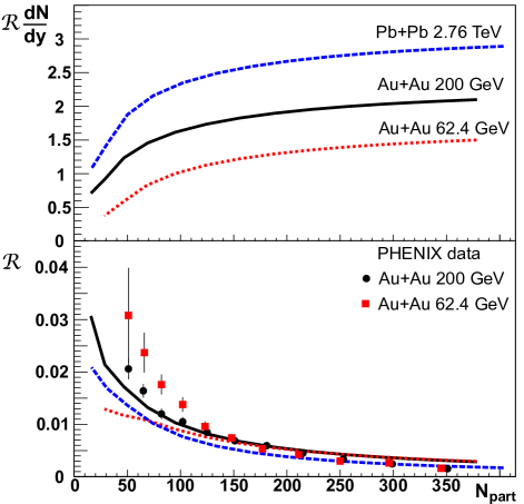
Figure 1: Prediction for ${\cal R}dN/dy$ as a function on the number of participants $N_{\rm part}$ at three beam energies (top). Calculated $\cal R$ compared to PHENIX data from Adare et al. (2008) (bottom).

PHENIX has measured multiplicity fluctuations at RHIC Adler et al. (2007); Adare et al. (2008). They report a negative binomial parameter $k_{{}_{NBD}}$. The best we can do is to compare their $k_{{}_{NBD}}^{-1}={\cal R}$ to (30) divided by $dN/dy$ measured elsewhere. Results shown in the lower panel in Fig. 1 agree fairly well in central collisions.

The experimental result that $\cal R$ is not zero shows that geometric shape variation is not the only source of fluctuations. To deduce anything beyond that, two caveats are in order. First, (29) and (30) strictly apply only to the number of gluons. Taking the number of particles to be conserved through hadronization as discussed in Ref. Kharzeev and Nardi (2001), we can identify $\cal R$ in (29) with the measured multiplicity fluctuations (7). However, one is then unsure how to address phenomenological concerns such as resonance decay. Second, experimenters must exercise care in measuring $\cal{R}$ as a function of centrality, because centrality selection can distort multiplicity fluctuations. Using narrow multiplicity bins to select centrality will remove fluctuations entirely. One way to remove this bias is to use a zero degree calorimeter to select centrality as PHENIX has done Adare et al. (2008). See the appendix for details.

An alternative probe of Glasma scaling is $\langle\delta p_{t1}\delta p_{t2}\rangle$. As with $\cal R$, the anisotropic flow contributions vanish on angular integration. The quantity $\langle\delta p_{t1}\delta p_{t2}\rangle$ is designed to be independent of multiplicity fluctuations, reducing our hadronization concerns Voloshin et al. (1999); Voloshin (2001). Moreover, it is effectively free of the multiplicity bias effect, as shown in the appendix. Unlike $\cal R$, momentum fluctuations depend on the scale of the fluid velocity because flow enhances $p_{t}$. We can constrain this dependence using $v_{2}$ and $\langle p_{t}\rangle$ measurements.

In order to calculate $\langle\delta p_{t1}\delta p_{t2}\rangle$ from (26) and (27) we must specify the relation between the initial transverse position $\mathbf{r}_{t}$ of a fluid cell and its final transverse flow velocity $\mathbf{v}_{t}$. To maintain consistency with our ridge analysis in Ref. Gavin et al. (2009); Moschelli and Gavin (2010), we use a blast wave model.

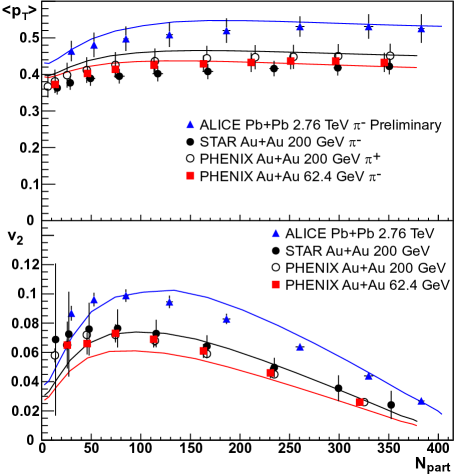
Figure 2: Average transverse momentum (top) and elliptic flow $v_{2}$ (bottom) as functions of $N_{\rm part}$ for the same energies as in Fig. 1. Mean $p_{t}$ data in GeV are from Adler et al. (2004); Abelev et al. (2009); Toia (2011) and $v_{2}$ data are from Shimimura (2009); Adams et al. (2005); Aamodt et al. (2011).

There we assumed $\gamma\mathbf{v}_{t}=\lambda\mathbf{r}_{t}$ and uniform temperature $T$, with parameters chosen to reproduce fits to 200 GeV Au+Au $p_{t}$ spectra Gavin et al. (2009); Moschelli and Gavin (2010). Sorensen et al.  subsequently pointed out the importance of allowing for the ellipticity of the source in describing the centrality dependence of the ridge Sorensen et al. (2011). To account for the ellipticity of the collision volume, we now take $\gamma\mathbf{v}_{t}=\lambda(\epsilon_{x}x\hat{x}+\epsilon_{y}y\hat{y})$, where $\epsilon_{x,y}^{2}=1\pm\epsilon$. The average $v_{t}$ and freeze out temperature in 62 GeV and 200 GeV Au+Au collisions are the same as those used in Gavin et al. (2009); Moschelli and Gavin (2010) and are based on an analysis in Kiyomichi (2005). At 2.76 TeV the velocity is scaled up from the 200 GeV values by 6% and the temperature is scaled up by 7%. We present these parameters in Fig. 3; note that the change in $v_{t}$ and $T$ with beam energy is rather small. The eccentricity $\epsilon$ is chosen to fit the observed centrality dependence of elliptic flow $v_{2}$ in 62 and 200 GeV Au+Au collisions and 2.76 TeV Pb+Pb collisions Shimimura (2009); Adams et al. (2005); Aamodt et al. (2011). The top panel in Fig. 2 compares these calculations to data from Refs. Adler et al. (2004); Abelev et al. (2009); Toia (2011). We then use (25) to compute $v_{2}$ and compare to $v_{2}\{2\}$, which includes fluctuations. To see how well these blast wave parameterizations work for the problem at hand, we calculate the average transverse momentum $\langle p_{t}\rangle=\int p_{t}\rho_{1}d\mathbf{p}/\int\rho_{1}d\mathbf{p}$ using (18). The agreement is shown in Fig. 2.

Figure 3: Blast-wave parameters for temperature (in GeV) and average velocity as functions of centrality. Data are from Ref. Kiyomichi (2005).

We now compute $\langle\delta p_{t1}\delta p_{t2}\rangle$. The multiplicity variance $\cal R$ is obtained from (30). We employ (26) and (27) combined with (17), and use the blast wave parameters discussed above. These are compared to data from Ref. Adams et al. (2005); Heckel (2011) in Fig. 4. The STAR collaboration at RHIC and the ALICE collaboration at LHC measure $\langle\delta p_{t1}\delta p_{t2}\rangle$ for charged particles rather than pions. There is little difference between these quantities at RHIC, but at LHC the $K/\pi$ and $p/\pi$ ratios are appreciably larger than expected in the observed range $0.15<p_{t}<2$  GeV Floris et al. . Using the measured $\langle p_{t}\rangle$ and particle ratios for kaons and protons gives $\langle p_{t}\rangle_{ch}/\langle p_{t}\rangle_{\pi}\sim 1.13$; PYTHIA gives $\sim 1.07$. The top solid curve in Fig. 4 is our computation with the measured $K/\pi$ and $p/\pi$ ratios, while the dashed curve assumes PYTHIA ratios. Agreement with data is very good for central collisions where our local equilibrium assumptions are most applicable. Deviations in peripheral collisions may be due in part to incomplete thermalization, see Gavin (2004, 2004).

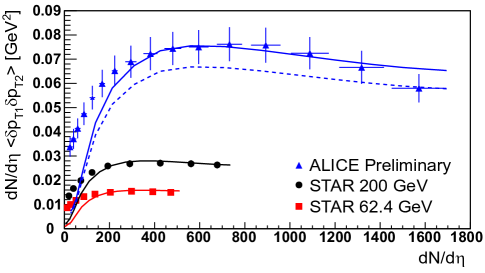
Figure 4: Transverse momentum fluctuations $\langle\delta p_{t1}\delta p_{t2}\rangle dN/d\eta$ as a function on the number of participants $N_{\rm part}$ at the same three beam energies. Data is from Adams et al. (2005); Heckel (2011). Dashed and solid 2.76 TeV curves represent different $K$ and $p$ contributions to charged particle fluctuations as discussed in the text.

VI Summary

In this paper we have studied the connection between long range correlations, fluctuations, and flow. While our results in Sec. V primarily address fluctuations, we discuss flow in Sec.  IV to establish its roll in correlations so that we can isolate its effect. As anticipated, our flow coefficients and their fluctuations given by (24) and (25) depend primarily on the spatial distribution of flux tubes – the “shape fluctuations” – described by the probability distribution $\rho_{{}_{FT}}$. Consequently, the relative magnitude of near and away-side features in $\Delta\phi$ correlations depends on these shape fluctuations. However, it is only in this relative sense that hydrodynamic response to initial shape fluctuations explains long range correlations Luzum (2011).

The scale of correlations $\cal{R}$ is important in comparing correlations at different centralities and energies. In particular, Refs. Gavin et al. (2009); Moschelli and Gavin (2010) compared calculations to the peak height of the ridge at $\Delta\phi=0$ for Au+Au and Cu+Cu collisions for a range of energies and kinematic conditions. Experimenters normalize the peak $\Delta\rho$ to the number of pairs from mixed events $\sqrt{\rho_{ref}}$. When jet and momentum conservation contributions are omitted, our results had the form $\Delta\rho/\sqrt{\rho_{ref}}={\cal R}(dN/dy)F(\Delta\phi)$, where $F$ depends only on flow. We found the beam-energy, centrality, and $A$ dependence of ${\cal R}$ to be consistent with data; see Moschelli and Gavin (2010) for details. To relate this to the current context, observe that the Fourier decomposition of $F$ gives (23). This supports the arguments regarding the physical significance of the height of the ridge stated in Dumitru et al. (2008); Gavin et al. (2009); Dusling et al. (2009); Moschelli and Gavin (2010). A limitation of Refs.  Dumitru et al. (2008); Gavin et al. (2009); Dusling et al. (2009); Moschelli and Gavin (2010) is that it is difficult to distinguish flow from Glasma effects when concentrating exclusively on the ridge.

Fluctuation studies provide an alternative set of experimental techniques for attacking correlation physics. In Sec. III we showed that multiplicity and $p_{t}$ fluctuations are independent of anisotropic flow. Measurement of such fluctuations remove much of the hydrodynamic uncertainty of ridge studies Dumitru et al. (2008); Gavin et al. (2009); Dusling et al. (2009); Moschelli and Gavin (2010). We emphasize that the mere fact that the measured $\cal R$ and $\langle\delta p_{t1}\delta p_{t2}\rangle$ are nonzero proves that event-wise variation of the initial geometric shape is not the only source of fluctuations.

In Sec. V we related the correlation strength to two fluctuation observables $\cal R$ and $\langle\delta p_{t1}\delta p_{t2}\rangle$. Glasma calculations of $\cal R$ in Fig. 1 and $\langle\delta p_{t1}\delta p_{t2}\rangle$ in Fig. 4 are in good accord with data, except for peripheral collisions. The deviation in peripheral collisions may reflect the breakdown of the assumption of local equilibrium. The onset of thermalization in peripheral collisions modifies the correlation function. In particular, this effect has been shown to modify $\langle\delta p_{t1}\delta p_{t2}\rangle$ at low numbers of participants Gavin (2004). Partial thermalization describes peripheral RHIC data very well and, moreover, allows one to describe $pp$ and $AA$ collisions in the same model Gavin (2004).

The fact that long range correlations can account for the measured $\langle\delta p_{t1}\delta p_{t2}\rangle$ leaves us with a puzzle. There are two types of fluctuations in nuclear collisions. First, each collision produces a different multi-particle system. Second, the partonic system produced in each event undergoes dynamic fluctuations as it evolves and hadronizes. We have focused on the source of long range correlations, where causality precludes the second type. However, fluctuation observables integrate both long and short range effects. Short range effects include jets and jet quenching, HBT, resonance decay, hadronization and hadro-chemical effects – not to mention novel fluctuations due to the phase transition. These effects modify correlations in the range $\Delta\eta\sim 1-2$ units or less. Jet-quenching, which most strongly affects central collisions, was estimated in Ref. Abdel-Aziz and Gavin (2005). Long range effects such as flow are charge independent. Net-charge fluctuations are therefore sensitive primarily to short range effects and, indeed, data show the appropriate rapidity dependence Abelev et al. (2009). Perhaps measurement of charge-dependent fluctuations, ${\cal R}_{ab}$ and $\langle\delta p_{t1}\delta p_{t2}\rangle_{ab}$ for $a,b=+$ or $-$, would help distinguish long range from short range contributions.

Appendix A Experimental Considerations

In this appendix we discuss experimental issues that affect the measurement of the fluctuation observables ${\cal R}$ and $\langle\delta p_{t1}\delta p_{t2}\rangle$. We show that biases can modify ${\cal R}$ if multiplicity is used to identify centrality in fluctuation observables, but that $\langle\delta p_{t1}\delta p_{t2}\rangle$ is largely unaffected. Experimental considerations in fluctuation measurements were discussed in Ref. Pruneau et al. (2002). These observables were constructed to be independent of experimental acceptance and efficiency effects, and many contributions that alter $\cal R$ were estimated. We extend the treatment in Ref.  Pruneau et al. (2002) to include $\langle\delta p_{t1}\delta p_{t2}\rangle$.

Assume that the collision produces $K$ independent ‘sources’ which then produce particles; one can think of each source as a flux tube or a wounded nucleon, depending on one’s favorite model. A set of events with fixed $K$ produces the single and pair densities that scale as:

$$\rho_{1}=\hat{\rho}_{1}K,\,\,\,\,\,\,\,\,\rho_{2}=\hat{\rho}_{2}K+\hat{\rho}_{1}\hat{\rho}_{1}K(K-1).$$ (31)

Suppose that experimenters measure a multiplicity $m$ to identify centrality. Each $m$ bin receives contributions from a range of $K$, so that the measured quantities are averaged over that ensemble. The multiplicity of a particular particle species will roughly satisfy $\langle N\rangle_{m}=\langle\int\rho_{1}\rangle_{m}\propto\langle K\rangle_{m}$. Equations (7), (9), and (31) imply that multiplicity fluctuations satisfy

$${\cal R}_{m}={{A}\over{\langle K\rangle_{m}}}+{{\langle K^{2}\rangle_{m}-\langle K\rangle_{m}^{2}}\over{\langle K\rangle_{m}^{2}}}.$$ (32)

where $A$ is a model-dependent constant, see Ref.  Pruneau et al. (2002) for details. The first term represents the average fluctuations per source. The second term comes from fluctuations in the number of sources. Unconstrained, independent sources follow Poisson statistics, $\langle K^{2}\rangle_{m}-\langle K\rangle_{m}^{2}=\langle K\rangle_{m}$.

To illustrate the effect of centrality cuts on ${\cal R}_{m}$, consider the following opposite extremes. Suppose for the moment that $m$ and $N$ are multiplicities measured in the same rapidity interval, so that one can approximate $m\propto K\propto N$. Then the fluctuations of $K$ for fixed $m$ vanish. On the other hand, if we take $m$ to be the signal in a zero degree calorimeter, then $m$ and $K$ are correlated only by the impact parameter $b$. Fluctuations of $K$ may then dominate (32) and be Poissonian Gavin et al. (2009).

We now consider transverse momentum fluctuations $\langle\delta p_{t1}\delta p_{t2}\rangle$. We combine (31) with (11), first noting that $\langle p_{t}\rangle=\int p_{t}\rho_{1}/\int\rho_{1}$ implies that $\int\rho_{1}\delta p_{t}\equiv 0$. Therefore, the numerator of (11) satisfies $\int\rho_{2}\delta p_{t1}\delta p_{t2}\propto\langle K\rangle_{m}$. The denominator of (11) is $\langle N(N-1)\rangle_{m}=\langle N\rangle_{m}^{2}(1+{\cal R}_{m})$. This implies that

$$\langle\delta p_{t1}\delta p_{t2}\rangle_{m}={{B}\over{\langle K\rangle_{m}}}\,{{1}\over{1+{\cal R}_{m}}},$$ (33)

where $B$ is another constant. This quantity has no additional contribution from $K$ fluctuations as in (32). However, a small centrality-bias effect may result from the ${\cal R}_{m}$ in the denominator.

To estimate this effect, observe that our CGC calculation gives ${\cal R}\sim 0.0017$ for central 2.76 GeV PbPb collisions, and 0.02 for the most peripheral value computed, which corresponds to $N_{\rm part}\approx 10$ participants. The effect of centrality bias on $\langle\delta p_{t1}\delta p_{t2}\rangle$ is therefore negligible. However, it might be important in pp collisions with a multiplicity trigger. Of course, the effect could be eliminated by normalizing to $\langle N\rangle^{2}$ rather than $\langle N(N-1)\rangle$, but that would have consequences regarding the cancellation of efficiencies.

References

- Putschke (2007) J. Putschke, J. Phys., G34, S679 (2007), arXiv:nucl-ex/0701074 .
- Abelev (2009) B. I. Abelev (STAR), (2009), arXiv:0909.0191 [nucl-ex] .
- Nattrass (2009) C. Nattrass, Eur. Phys. J., C62, 265 (2009), arXiv:0809.5261 [nucl-ex] .
- Daugherity (2008) M. Daugherity (STAR), J. Phys., G35, 104090 (2008), arXiv:0806.2121 [nucl-ex] .
- De Silva (2009) L. De Silva (STAR), (2009), arXiv:0910.5938 [nucl-ex] .
- Adams et al. (2006) J. Adams et al. (STAR), J. Phys., G32, L37 (2006), arXiv:nucl-ex/0509030 .
- Adamova et al. (2008) D. Adamova et al. (CERES), Nucl.Phys., A811, 179 (2008), arXiv:0803.2407 [nucl-ex] .
- Alver et al. (2008) B. Alver et al. (PHOBOS), J. Phys., G35, 104080 (2008), arXiv:0804.3038 [nucl-ex] .
- Alver et al. (2009) B. Alver et al. (PHOBOS), (2009), arXiv:0903.2811 [nucl-ex] .
- Alver and Roland (2010) B. Alver and G. Roland, Phys. Rev., C81, 054905 (2010), arXiv:1003.0194 [nucl-th] .
- Takahashi et al. (2009) J. Takahashi et al., Phys. Rev. Lett., 103, 242301 (2009), arXiv:0902.4870 [nucl-th] .
- Alver et al. (2010) B. H. Alver, C. Gombeaud, M. Luzum, and J.-Y. Ollitrault, Phys. Rev., C82, 034913 (2010), arXiv:1007.5469 [nucl-th] .
- Sorensen (2010) P. Sorensen, J.Phys.G, G37, 094011 (2010), arXiv:1002.4878 [nucl-ex] .
- Sorensen et al. (2011) P. Sorensen, B. Bolliet, A. Mocsy, Y. Pandit, and N. Pruthi, (2011), arXiv:1102.1403 [nucl-th] .
- Luzum (2010) M. Luzum, (2010), arXiv:1011.5773 [nucl-th] .
- Petersen et al. (2010) H. Petersen, C. Coleman-Smith, S. A. Bass, and R. Wolpert, (2010).
- Qin et al. (2010) G.-Y. Qin, H. Petersen, S. A. Bass, and B. Muller, Phys.Rev., C82, 064903 (2010), arXiv:1009.1847 [nucl-th] .
- Petersen and Bleicher (2010) H. Petersen and M. Bleicher, Phys.Rev., C81, 044906 (2010), arXiv:1002.1003 [nucl-th] .
- Teaney and Yan (2010) D. Teaney and L. Yan, (2010), arXiv:1010.1876 [nucl-th] .
- Schenke et al. (2011) B. Schenke, S. Jeon, and C. Gale, Phys. Rev. Lett., 106, 042301 (2011), arXiv:1009.3244 [hep-ph] .
- Qiu and Heinz (2011) Z. Qiu and U. W. Heinz, (2011), arXiv:1104.0650 [nucl-th] .
- Westfall (2008) G. D. Westfall, J.Phys.G, G35, 104031 (2008).
- Koch (2008) V. Koch, (2008), arXiv:0810.2520 [nucl-th] .
- Aggarwal et al. (2010) M. M. Aggarwal et al. (STAR), (2010), arXiv:1007.2613 [nucl-ex] .
- Gavin (2004) S. Gavin, Phys. Rev. Lett., 92, 162301 (2004a), arXiv:nucl-th/0308067 .
- Gavin (2004) S. Gavin, J. Phys., G30, S1385 (2004b), arXiv:nucl-th/0404048 .
- Voloshin (2006) S. A. Voloshin, Phys.Lett., B632, 490 (2006), arXiv:nucl-th/0312065 [nucl-th] .
- Mrowczynski et al. (2004) S. Mrowczynski, M. Rybczynski, and Z. Wlodarczyk, Phys.Rev., C70, 054906 (2004), arXiv:nucl-th/0407012 [nucl-th] .
- Broniowski et al. (2009) W. Broniowski, M. Chojnacki, and L. Obara, Phys. Rev., C80, 051902 (2009), arXiv:0907.3216 [nucl-th] .
- Pruneau et al. (2002) C. Pruneau, S. Gavin, and S. Voloshin, Phys. Rev., C66, 044904 (2002), arXiv:nucl-ex/0204011 .
- Dumitru et al. (2008) A. Dumitru, F. Gelis, L. McLerran, and R. Venugopalan, Nucl. Phys., A810, 91 (2008), arXiv:0804.3858 [hep-ph] .
- Gavin et al. (2009) S. Gavin, L. McLerran, and G. Moschelli, Phys.Rev., C79, 051902 (2009), arXiv:0806.4718 [nucl-th] .
- Moschelli and Gavin (2010) G. Moschelli and S. Gavin, Nucl.Phys., A836, 43 (2010), arXiv:0910.3590 [nucl-th] .
- Dusling et al. (2009) K. Dusling, D. Fernandez-Fraile, and R. Venugopalan, Nucl. Phys., A828, 161 (2009a), arXiv:0902.4435 [nucl-th] .
- Pruneau et al. (2008) C. A. Pruneau, S. Gavin, and S. A. Voloshin, Nucl. Phys., A802, 107 (2008), arXiv:0711.1991 [nucl-ex] .
- Lindenbaum and Longacre (2007) S. J. Lindenbaum and R. S. Longacre, Eur. Phys. J., C49, 767 (2007).
- Peitzmann (2009) T. Peitzmann, (2009), arXiv:0903.5281 [nucl-th] .
- Andrade et al. (2010) R. P. G. Andrade, F. Grassi, Y. Hama, and W.-L. Qian, (2010), arXiv:1008.4612 [nucl-th] .
- Werner et al. (2010) K. Werner, I. Karpenko, T. Pierog, M. Bleicher, and K. Mikhailov, (2010), arXiv:1004.0805 [nucl-th] .
- Sharma et al. (2011) M. Sharma et al., (2011), arXiv:1107.3587 [nucl-th] .
- Voloshin et al. (2008) S. A. Voloshin, A. M. Poskanzer, and R. Snellings, (2008), arXiv:0809.2949 [nucl-ex] .
- Sorensen (2009) P. Sorensen, (2009), arXiv:0905.0174 [nucl-ex] .
- Dusling et al. (2009) K. Dusling, F. Gelis, T. Lappi, and R. Venugopalan, (2009b), arXiv:0911.2720 [hep-ph] .
- Borghini et al. (2002) N. Borghini, P. M. Dinh, J.-Y. Ollitrault, A. M. Poskanzer, and S. A. Voloshin, Phys. Rev., C66, 014901 (2002), arXiv:nucl-th/0202013 .
- Borghini (2003) N. Borghini, Eur. Phys. J., C30, 381 (2003), arXiv:hep-ph/0302139 .
- Borghini (2007) N. Borghini, Phys. Rev., C75, 021904 (2007a), arXiv:nucl-th/0612093 .
- Borghini (2007) N. Borghini, PoS, LHC07, 013 (2007b), arXiv:0707.0436 [nucl-th] .
- Chajecki and Lisa (2008) Z. Chajecki and M. Lisa, Phys. Rev., C78, 064903 (2008), arXiv:0803.0022 [nucl-th] .
- Luzum (2011) M. Luzum, (2011), arXiv:1107.0592 [nucl-th] .
- Gazdzicki and Mrowczynski (1992) M. Gazdzicki and S. Mrowczynski, Z.Phys., C54, 127 (1992).
- Mrowczynski (1998) S. Mrowczynski, Phys.Lett., B439, 6 (1998), arXiv:nucl-th/9806089 [nucl-th] .
- Voloshin et al. (1999) S. Voloshin, V. Koch, and H. Ritter, Phys.Rev., C60, 024901 (1999), arXiv:nucl-th/9903060 [nucl-th] .
- Voloshin (2001) S. A. Voloshin (STAR), , 591 (2001), arXiv:nucl-ex/0109006 [nucl-ex] .
- Adamova et al. (2003) D. Adamova et al. (CERES), Nucl.Phys., A727, 97 (2003), arXiv:nucl-ex/0305002 [nucl-ex] .
- Adams et al. (2005) J. Adams et al. (STAR), PHRVA,C72,044902.2005, C72, 044902 (2005a), arXiv:nucl-ex/0504031 [nucl-ex] .
- Gavin and Abdel-Aziz (2006) S. Gavin and M. Abdel-Aziz, Phys. Rev. Lett., 97, 162302 (2006), arXiv:nucl-th/0606061 .
- Bhalerao et al. (2011) R. S. Bhalerao, M. Luzum, and J.-Y. Ollitrault, (2011), arXiv:1104.4740 [nucl-th] .
- Kharzeev and Nardi (2001) D. Kharzeev and M. Nardi, Phys. Lett., B507, 121 (2001), arXiv:nucl-th/0012025 .
- Gelis et al. (2009) F. Gelis, T. Lappi, and L. McLerran, Nucl. Phys., A828, 149 (2009), arXiv:0905.3234 [hep-ph] .
- Adare et al. (2008) A. Adare et al. (PHENIX), Phys. Rev., C78, 044902 (2008), arXiv:0805.1521 [nucl-ex] .
- Adler et al. (2007) S. S. Adler et al. (PHENIX), Phys. Rev., C76, 034903 (2007), arXiv:0704.2894 [nucl-ex] .
- Adler et al. (2004) S. S. Adler et al. (PHENIX), Phys. Rev., C69, 034909 (2004), arXiv:nucl-ex/0307022 .
- Abelev et al. (2009) B. I. Abelev et al. (STAR), Phys. Rev., C79, 034909 (2009a), arXiv:0808.2041 [nucl-ex] .
- Toia (2011) A. Toia (ALICE), (2011), arXiv:1107.1973 [nucl-ex] .
- Shimimura (2009) M. Shimimura, Systematic Study of Azimuthal Anisotropy for Charged Hadron in Relativistic Nucleus-Nucleus Collisions at RHIC-PHENIX, Ph.D. thesis (2009).
- Adams et al. (2005) J. Adams et al. (STAR), Phys. Rev., C72, 014904 (2005b), arXiv:nucl-ex/0409033 .
- Aamodt et al. (2011) K. Aamodt et al. (ALICE), (2011), arXiv:1105.3865 [nucl-ex] .
- Kiyomichi (2005) A. Kiyomichi, Study of identified hadron spectra and yields at mid- rapidity in s(NN)**(1/2) = 200-GeV Au + Au collisions, Ph.D. thesis (2005).
- Heckel (2011) S. Heckel (ALICE), Talk at Quark Matter 2011, Annecy, France (2011), arXiv:1107.4327 [nucl-ex] .
- (70) M. Floris et al. (ALICE), Talk at Quark Matter 2011, Annecy, France.
- Abdel-Aziz and Gavin (2005) M. Abdel-Aziz and S. Gavin, Int.J.Mod.Phys., A20, 3786 (2005).
- Abelev et al. (2009) B. I. Abelev et al. (STAR), Phys. Rev., C79, 024906 (2009b), arXiv:0807.3269 [nucl-ex] .