Abstract

We study quantum frequency translation and two-color photon interference enabled by the Bragg scattering four-wave mixing process in optical fiber. Using realistic model parameters, we computationally and analytically determine the Green function and Schmidt modes for cases with various pump-pulse lengths. These cases can be categorized as either “non-discriminatory” or “discriminatory” in regards to their propensity to exhibit high-efficiency translation or high-visibility two-photon interference for many different shapes of input wave packets or for only a few input wave packets, respectively. Also, for a particular case, the Schmidt mode set was found to be nearly equal to a Hermite-Gaussian function set. The methods and results also apply with little modification to frequency conversion by sum-frequency conversion in optical crystals.

OCIS codes: (000.4430) Numerical approximation and analysis; (190.4380) Four-wave mixing; (270.5585) Quantum information and processing

1 Introduction

Quantum frequency translation (QFT) is the process whereby two spectral modes (or narrow bands of modes) are swapped in the sense that the properties of their quantum states (other than their central frequencies) are interchanged, as in Fig. 1 [1, 2, 3]. Such a process, of course, requires an external source or sink of energy, which is provided by a strong external optical field. Ideally, an arbitrary state of the narrow band of green modes will be swapped with the state of the narrow band of blue modes. These could be coherent, squeezed, or number states, and may also be entangled with other, separate degrees of freedom, such as other modes (e.g., violet and yellow) or states of atoms, quantum dots, etc. When the states of the green and blue modes are swapped, the prior entanglement should be preserved. This paper focuses on the QFT of single-photon states.

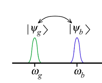
Fig. 1: Quantum frequency translation of wavepacket states between green and blue spectral regions. The states being translated could be coherent, squeezed, or number states.

QFT is defined to be “noiseless,” that is, free of excess background noise. For example, if both modes to be swapped are initially vacuum, they should remain vacuum$-$there are no spontaneous processes that can populate modes in this case. The noiseless property distinguishes QFT from other frequency conversion processes such as optical parametric amplification, which has been widely studied for use in classical telecom systems [4, 5, 6]. In optical parametric amplification, power is spontaneously transferred from the pump(s) to the weak signal fields, and without any blue input power, the signal fields can build up spontaneously.

The QFT capability will play important roles in quantum information science (QIS), where states of a quantum memory may be transmitted to a spatially remote quantum memory by emitting and absorbing photons. If the two memories operate using distinct frequencies of their absorption/emission lines, it is necessary to “translate” the communication photons between these frequencies. Such a translation capability also allows sending the photons through low-loss optical fiber at wavelengths near 1500 nm, even in cases where the memories operate at other wavelengths.

Two methods for all-optical QFT have been demonstrated: three-wave mixing in a second-order nonlinear optical medium (crystal) [2, 7] and more recently four-wave mixing (FWM) in a third-order nonlinear optical medium (silica fiber) [8]. In the case of three-wave mixing and referring to Fig. 1, the strong pump field must have frequency $\omega_{p}=\omega_{b}-\omega_{g}$. The configuration for FWM with two pumps, denoted $p$ and $q$, is that of dynamic Bragg scattering, in which for example, one photon is removed from pump $p$ and one is added to pump $q$. At the same time, one photon is removed from the green signal and one is added to the blue signal so that $\omega_{p}+\omega_{g}=\omega_{q}+\omega_{b}$. This contrasts with optical parametric amplification, wherein photons are removed from the pump(s) and photons are added to both signals.

Experiments have included QFT of one-half of a number-correlated state [7] and several examples of QFT of single-photon states by three-wave mixing in crystals [1, 2, 9] and by FWM in fiber [8]. The main advantage of the FWM method over the three-wave mixing method is that it allows QFT between spectral bands separated by large or small shifts, whereas in practice three-wave mixing allows QFT only between far-separated bands [8]. This paper treats the theory of FWM, but the same methods can easily be applied to three-wave mixing.

A potentially revolutionary application of QFT is that it is predicted to enable the interference of two photons (or other states of the modes) with different colors [10]. This phenomenon generalizes the famous Hong-Ou-Mandel (HOM) interference effect, wherein two photons of like color and identical wave-packet structure impinge simultaneously on a standard beam splitter. Because of the boson nature of photons, the beam-splitter output modes both contain either zero or two photons, but never one photon in each. This remarkable effect (which is analogous to the exchange interaction for electrons) enables a class of quantum information processing known as linear-optical quantum computing [11], including many variants [12].

The promise of QFT is that it offers the possibility to perform linear-optical quantum computing “over the rainbow.” That is, one could use the light’s color as a degree of freedom identifying optical qubits and perform linear-optical quantum computing using the generalization of the HOM effect involving distinct frequencies. This would entail creating entangled states involving many distinct frequencies (perhaps by methods such as in [13, 14]), and manipulating such states using two-mode interference via QFT. This would require QFT between modes nearby in frequency, and so FWM would be greatly preferred over three-wave mixing. Other tools proposed for linear-optical quantum computing “over the rainbow” are temporal-mode filters (“pulse gates” [15] which could be used as channel add/drop filters in an optical communications system [16, 17]) and single-photon pulse shapers [18, 19], based on QFT by three-wave mixing.

In this paper we extend our earlier treatments [3, 10] to enable the explicit modeling of QFT by FWM in optical fiber or by three-wave mixing in a crystal. The treatment includes analytical and numerical components, and allows us to model realistically the effects of finite pulse durations, linear dispersion, finite phase-matching bandwidth, and complicating effects such as self-phase modulation (SPM) and cross-phase modulation (CPM) [20]. Previous theories of QFT have either assumed single-mode fields [3], disallowing rigorous treatment of pulse propagation, or assumed that the signal pulse shapes are not altered significantly by the translation process [15, 18, 19], obscuring the accurate design of high-fidelity devices.

The main results of this study are the following: We find that for realistic fiber and laser pulse parameters, essentially 100 percent efficient QFT can, in principle, be achieved. We show that for given temporal shapes of the pump pulses, usually there are unique shapes that the two signal wave packets should have in order that they be swapped optimally by QFT. These shapes are found as the optimal modes of a singular-value (Schmidt) decomposition of the Green function for the QFT process, and the shapes change significantly with changing translation efficiency. This result provides a method for designing QFT and two-photon interference with high efficiency and high fidelity. We also show, for a given pump temporal shape, how to design signal pulse shapes to create perfect HOM interference via the FWM process, as first predicted in [10].

2 Theory

The physical mechanism used to carry out frequency translation in fiber is the Bragg scattering (BS) four-wave mixing process [4, 8, 21], pictured in Fig. 2. For convenience, we refer to the two weak signal fields as “green” and “blue,” although in principle their actual frequencies could correspond to visible or near-IR radiation. Two strong pump fields drive the process in which one photon from one of the pumps, pump $p$ in Fig. 2, and one photon in the green field are annihilated while one photon from the other pump (denoted $q$) and one photon in the blue field are created. The process conserves photon number in accordance with the Manley-Rowe relations [22] and can be summarized as $\gamma_{p}+\gamma_{g}\rightarrow\gamma_{q}+\gamma_{b}$, where $\gamma$ represents a photon.

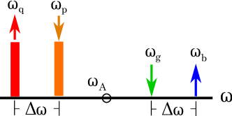
Fig. 2: BS process where the pumps have frequencies $\omega_{p}$ and $\omega_{q}$ and the signals have frequencies $\omega_{g}$ and $\omega_{b}$, where $\omega_{p}+\omega_{g}=\omega_{q}+\omega_{b}$. The arrows symbolize either annihilation (down) or creation (up) of a photon in that mode. The frequency $\omega_{A}$ is the average value of all the frequencies and $\Delta\omega$ is the frequency separation between the pump fields and also between the signal fields.

Before describing the realistic continuous-frequency case, we discuss a much simpler model in which each field is represented by a single-frequency mode. Such a model might apply to fields in a cavity, but strictly speaking not to the pulse propagation scenario in which we are interested. The simple model has the advantage of permitting analytical solutions, thereby providing some insight into the QFT process [3]. For cases where each field can be described by a single-frequency mode, the Hamiltonian governing the process is given by

$$\mathcal{H}=\Delta\beta(a^{\dagger}_{g}a_{g}-a^{\dagger}_{b}a_{b})/2+\kappa a^{\dagger}_{g}a_{b}+\kappa^{*}a^{\dagger}_{b}a_{g},$$ (1)

where the creation/annihilation operators satisfy the usual commutation relations, and $\Delta\beta$ and $\kappa$ are parameters quantifying the effects of phase-mismatch and nonlinearity [3]. The evolution is given by the spatial equations-of-motion (with a minus sign compared to the usual time-domain Heisenberg equation)

$$\frac{d}{dz}a_{b(g)}(z)=i[a_{b(g)}(z),\mathcal{H}].$$ (2)

The solution of (2) for $a_{g(b)}(z)$ as a function of position along the fiber $z$ for a fiber of length $L$ is given by

$$a_{g}(z) =\mu(z)a_{g}(0)+\nu(z)a_{b}(0),$$ (3)

$$a_{b}(z) =\mu^{*}(z)a_{b}(0)-\nu^{*}(z)a_{g}(0),$$ (4)

where the “transfer” functions are given by

$$\mu(z) =\textrm{cos}(kz)+i\Delta\beta\textrm{sin}(kz)/2k,$$ (5)

$$\nu(z) =i\kappa\;\textrm{sin}(kz)/k,$$ (6)

where $k=(\Delta\beta^{2}/4+|\kappa|^{2})^{1/2}$. The transfer functions have the relation $|\mu|^{2}+|\nu|^{2}=1$, which ensures the process is unitary and conserves photon number. Mathematically, the BS translation process having frequency input and output “ports” is identical to the normal beam-splitter operation on degenerate monochromatic fields [23]. For perfect translation from green to blue, and vice versa, it must be that $|\nu(L)|=1$ for a medium of length $L$. In this case the quantum states of the modes are completely swapped. For example, a single green photon is replaced by a single blue photon, that is, $|1,0\rangle\rightarrow|0,1\rangle$, where $|i,j\rangle$ denotes the state in which $i$ photons are in the green region and $j$ photons are in the blue region.

Since the BS process is analogous to beamsplitter action, all of the effects that a beamsplitter can induce on a field will also occur in the BS process. In particular, the effect analogous to two-photon HOM interference will occur, where two independent photons of differing frequencies will interfere with one another and give a perfect HOM dip under the appropriate circumstances [10]. Just as in the monochromatic HOM interference effect, the “frequency beamsplitter” must have equal transmission and reflection coefficients, that is $|\mu|^{2}=|\nu|^{2}=1/2$, so that it is equally likely for the blue (green) photon to stay in the blue (green) mode or be translated to the green (blue) mode. Using the above equations it can be shown that in this case, for an input state consisting of one green photon and one blue photon, denoted by $a_{g}^{\dagger}(0)a_{b}^{\dagger}(0)|\rm{vac}\rangle=|1,1\rangle_{\rm{in}}$, the output state is given by

$$|1,1\rangle_{\rm{in}}=\left([|\mu|^{2}-|\nu|^{2}]|1,1\rangle_{\rm{out}}+\sqrt{2}\mu\nu|2,0\rangle_{\rm{out}}-\sqrt{2}\mu^{*}\nu^{*}|0,2\rangle_{\rm{out}}\right).$$ (7)

For equal values of $|\mu|^{2}$ and $|\nu|^{2}$ the $|1,1\rangle$ component of the state cancels to zero.

The above analysis is valid only if all the fields involved are single-mode. For fields that contain multiple-frequency components, as any pulsed field does, the theory becomes much more complex. For arbitrary input, and even “simple” multi-mode input such as Gaussian pulses, the output cannot in general be determined analytically. However, it is possible to assign analytically a Green function $G$ in either frequency $\omega$ or time $t$ that relates the input wavepacket to the output wavepacket for arbitrary input, analogous to (3) and (4), for given pump spectra, fiber dispersion, and fiber length [10]. Denoting the creation operator at position $z$ by $a^{\dagger}(z,\omega)$, the input $a^{\dagger}(0,\omega)$, and output $a^{\dagger}(L,\omega)$ are related by the forward transformation

$$a^{\dagger}(L,\omega)=\int d\omega^{{}^{\prime}}G^{*}(\omega^{{}^{\prime}},\omega)a^{\dagger}(0,\omega^{{}^{\prime}}).$$ (8)

For our purposes, the backward transformation is more useful:

$$a^{\dagger}(0,\omega)=\int d\omega^{{}^{\prime}}G(\omega,\omega^{{}^{\prime}})a^{\dagger}(L,\omega^{{}^{\prime}}),$$ (9)

which gives the input operator in terms of an integral over the output operator.

A single-photon input wavepacket given by $\int d\omega A(0,\omega)a^{\dagger}(0,\omega)|vac\rangle$, where $A(0,\omega)$ is the spectrum of the input wavepacket, is translated in the manner given by (9). The state can thus be expressed in terms of the output operator as

$$|\psi\rangle=\int d\omega A(0,\omega)\int d\omega^{{}^{\prime}}G(\omega,\omega^{{}^{\prime}})a^{\dagger}(L,\omega^{{}^{\prime}})|vac\rangle.$$ (10)

The Green function is unitary and therefore satisfies the condition

$$\int d\omega^{{}^{\prime}}G(\omega,\omega^{{}^{\prime}})G^{*}(\omega^{{}^{\prime\prime}},\omega^{{}^{\prime}})=\delta(\omega-\omega^{{}^{\prime\prime}}).$$ (11)

To facilitate an intuitive understanding of the transfer function, we break up frequency space into two pieces; the range that contains the green and the range that contains the blue. Each operator or variable will be denoted by a “$g$” or “$b$” subscript. For example, the creation operator for an green photon at a particular green frequency will be written as $a^{\dagger}_{g}(\omega_{g})$. In this case the transfer function can be written in block form as [10]

$$\left[\begin{array}[]{cc}G_{gg}(\omega_{g},\omega_{g}^{{}^{\prime}})&G_{gb}(\omega_{g},\omega_{b}^{{}^{\prime}})\\ G_{bg}(\omega_{b},\omega_{g}^{{}^{\prime}})&G_{bb}(\omega_{b},\omega_{b}^{{}^{\prime}})\end{array}\right]$$ (12)

where $G_{xy}$ refers to the evolution of an output creation operator in range $y$ which came from range $x$.

Although the $G$ function completely describes the evolution of arbitrary inputs, it is difficult to discover which input pulses give rise to desirable effects such as high-efficiency translation or good two-color HOM interference just by examining the $G$ function. However, by performing a Schmidt (singular-value) decomposition (SVD) [24] on the $G$ function or on the sub-matrices $G_{xy}$, the input wavefunctions necessary to achieve these effects can be found [10]. For example, consider the translation of an input green field to the blue field, which is described by the Green sub-matrix by $G_{gb}$, which is not Hermitian and therefore does not admit a unitary decomposition. We write $G_{gb}$ in its SVD form as

$$G_{gb}(\omega,\omega^{{}^{\prime}})=-\sum_{n}\rho_{n}V_{n}(\omega)w_{n}^{*}(\omega^{{}^{\prime}}),$$ (13)

where the $\rho_{n}$ are the real, positive singular values (the generalization of eigenvalues), and $V_{n}$ and $w_{n}$ are the $n$th column vectors of the unitary “matrices” $V$ and $w$ describing the decomposition, respectively. The most useful way to interpret this decomposition is that a given green wavepacket $V_{n}$ will be translated to the blue wavepacket $w_{n}$ with probability $\rho_{n}^{2}$. Hence, only input green wavepackets $V_{n}$ that have associated singular values $\rho_{n}=1$ will translate over to the blue mode with 100 percent probability. The $G_{gg}$ “matrix” describes an input green wavepacket scattering within the green spectral region at the output (no translation from green to blue, although the shape of the wavepacket may change). If the SVD of $G_{gg}$ is given by [10]

$$G_{gg}(\omega,\omega^{{}^{\prime}})=\sum_{n}\tau_{n}V_{n}(\omega)\upsilon_{n}^{*}(\omega^{{}^{\prime}}),$$ (14)

then $\tau_{n}^{2}$ is the probability that an input green wavepacket $V_{n}$ will scatter to an output green wavepacket $\upsilon_{n}$ (the $V$ matrix here being the same as in the $G_{gb}$ decomposition). The singular values satisfy the relation $\tau_{n}^{2}+\rho_{n}^{2}=1$, as they must to conserve photon number.

Similarly, the $G_{bg}$ and $G_{bb}$ have their own SVDs, given by

$$G_{bg}(\omega,\omega^{{}^{\prime}}) =\sum_{n}\rho_{n}W_{n}(\omega)\upsilon_{n}^{*}(\omega^{{}^{\prime}}),$$ (15)

$$G_{bb}(\omega,\omega^{{}^{\prime}}) =\sum_{n}\tau_{n}W_{n}(\omega)w_{n}^{*}(\omega^{{}^{\prime}}),$$ (16)

where the $w$ and $\upsilon$ matrices, and the singular values $\tau$ and $\rho$, are the same as in (13) and (14). This highlights the interconnectedness between the various sub-Green functions in that there are only four unique Schmidt modes for each index $n$ that completely describe the process. Before treating exclusively single-photon inputs, we emphasize that the Green functions determined by our present approach can be used to treat arbitrary multi-photon inputs as well.

The SVD technique can be used to discover what input wavepackets are suitable for optimal two-photon HOM interference [10]. The condition is somewhat intuitive. Since in the single-mode, two-color case it is necessary for both green and blue inputs to have a 50 percent probability of translating to the other mode for perfect HOM interference, it is reasonable to guess this condition is also true in the multi-mode two-color case. Hence for the cases in which $\tau_{n}^{2}=\rho_{n}^{2}=1/2$, the corresponding input vectors $V_{n}$ and $W_{n}$ will show perfect two-color HOM interference. Alternatively, this condition can be written as

$$\sigma_{n}=2\tau_{n}\rho_{n}=1,$$ (17)

We refer to the quantity $\sigma_{n}=2\tau_{n}\rho_{n}$ as the HOM singular value, because it appears as such for a Schmidt decomposition kernel designed specifically to optimize the HOM interference. (See Eq. (37) of [10].) The closer it is to unity, the better the HOM interference.

There is an alternative, complimentary, method to calculate the degree of HOM interference that a BS process will exhibit, for which the Green function does not have to be calculated. First, consider the case in which there are two photons, either of which could be in the green or blue region, or in some superposition of both regions. In general, the state of this bi-photon can be written as

$$|\psi\rangle=C_{11}|1,1\rangle+C_{20}|2,0\rangle+C_{02}|0,2\rangle.$$ (18)

The entire state $|\psi\rangle$ must be normalized and the component states are orthonormal. Now, for input consisting of one green photon and one blue photon having input spectra of $A_{g}(0,\omega_{g})$ and $A_{b}(0,\omega_{b})$ respectively, the state is

$$\int d\omega_{g}d\omega_{b}A_{g}(0,\omega_{g})A_{b}(0,\omega_{b})a_{g}^{\dagger}(0,\omega_{g})a_{b}^{\dagger}(0,\omega_{b})|vac\rangle.$$ (19)

If the photons undergo the BS process, the input photon operators evolve according to (9). By switching the limits of integration and noting that $\left[\int d\omega A_{X}(0,\omega)G^{*}_{XY}(\omega,\omega_{Y})\right]\rightarrow A_{XY}(L,\omega_{Y})$, where both $X$ and $Y$ could be either $g$ or $b$ and $A_{XY}(L,\omega_{Y})$ is a component of the spectrum at the output of the fiber, the state can be written compactly as

$$\begin{split}|\psi\rangle=&\big{[}\int d\omega_{g}a_{g}^{\dagger}(L,\omega_{g})A_{gg}(L,\omega_{g})+\int d\omega_{S}a_{b}^{\dagger}(L,\omega_{b})A_{bg}(L,\omega_{b})\big{]}\\ &\times\big{[}\int d\omega_{g}^{{}^{\prime}}a_{g}^{\dagger}(L,\omega_{g}^{{}^{\prime}})A_{gb}(L,\omega_{g}^{{}^{\prime}})+\int d\omega_{b}^{{}^{\prime}}a_{b}^{\dagger}(L,\omega_{b}^{{}^{\prime}})A_{bb}(L,\omega_{b}^{{}^{\prime}})\big{]}|vac\rangle.\end{split}$$ (20)

The probability, given a particular output state, for the various sub-space states to occur is given by the modulus squared of the coefficients of these states, $|C_{ij}|^{2}$. For the $|1,1\rangle$ state the coefficient is found by acting the aforementioned operators, with their accompanying functions, on the vacuum, yielding

$$|\psi_{11}\rangle=\int\int d\omega_{g}d\omega_{b}\left[A_{gg}(L,\omega_{g})A_{bb}(L,\omega_{b})+A_{gb}(L,\omega_{g})A_{bg}(L,\omega_{b})\right]|1_{\omega_{g}},1_{\omega_{b}}\rangle$$ (21)

The first term, $A_{gg}(L,\omega_{g})A_{bb}(L,\omega_{b})$, corresponds to the case where a photon initially in the green mode (i.e. wavepacket) scatters within the green mode at the output, and a photon initially in the blue mode scatters within the blue mode at the output. The second term, $A_{gb}(L,\omega_{g})A_{bg}(L,\omega_{b})$, corresponds to the case where a photon initially in the green mode scatters to the blue mode at the output, and a photon initially in the blue mode scatters to the green mode at the output. Since these terms are being added before their modulus squared is taken, there is the chance that they could cancel if the terms are proportional and out of phase with one another. This is exactly what happens in the case in which ideal HOM interference occurs, leaving zero probability amplitude for the field to emerge in the $|1,1\rangle$ state. The expression for the probability for this state to occur $P_{11}$ is

$$\begin{split}P_{11}=\int\int d\omega_{g}d\omega_{b}&\big{[}|A_{gg}(L,\omega_{g})|^{2}|A_{bb}(L,\omega_{b})|^{2}+|A_{gb}(L,\omega_{g})|^{2}|A_{bg}(L,\omega_{b})|^{2}+\\ &2\mathrm{Re}[A_{gg}(L,\omega_{g})A_{bb}(L,\omega_{b})A_{gb}^{*}(L,\omega_{g})A_{bg}^{*}(L,\omega_{b})|]\big{]}.\end{split}$$ (22)

This gives an expression to calculate the coincidence probability for any given input pulses without knowing the Green function for the process. In the alternative case in which we launch particular Schmidt modes as input signals, we showed previously that the coincidence count rate equals $P_{11}=(\tau_{n}^{2}-\rho_{n}^{2})^{2}$ [10]. Therefore, in this case we have a simple relation between $P_{11}$ and the HOM singular values; $P_{11}+\sigma_{n}^{2}=1$. Other important quantities are $P_{20}$ and $P_{02}$, the probabilities that two photons appear in one or the other output ports together. The expressions for these, and their derivation can be found in Appendix A.

3 Numerical implementation

Unfortunately, it is not possible to discover the Green function and its Schmidt modes by examining the Hamiltonian directly. One must solve for the full propagation first, then examine the input-output relations. This emphasizes that the Schmidt modes are global properties, depending on the entire evolution. For example, the input Schmidt modes depend on the length of the medium.

The appropriate Hamiltonian generates the well-known nonlinear Schrodinger equation, which needs to be solved. In most realistic circumstances, taking into account actual field shapes and real fiber dispersion properties, it is not possible to solve the nonlinear Schr$\ddot{\textrm{o}}$dinger equation for the fields analytically. So we turn to numerical computation to determine the evolution of a completely specified input state to a completely determined output state. The key difficulty with such an approach is that, in general, nonlinear operator equations cannot be simulated by any simple numerical scheme. When the evolution is both in space and time as in our case, the problem becomes one suited for techniques such as the positive-P representation [25, 26]. Fortunately, in our case, although the evolution is nonlinear in the pump fields, it is linear in the weak signal fields. This allows a simplification if we treat the pump fields as classically evolving parameters in the quantum Heisenberg equations of motion for the weak signals. Then the field operators for the weak signals can be solved in terms of Green functions that obey the classical evolution equations. Therefore, we solve numerically for the classical evolution of the Green functions and use those solutions to calculate any quantum probability or correlation function concerning the signal fields. An analogous procedure was used in [27, 28].

The usual starting point for solving for the nonlinear evolution of a pulse is to write the total field as $E(z,t)=A(z,t)e^{i(\beta_{0}z-\omega_{0}t)}$, where $A(z,t)$ is a slowly varying envelope function, $\omega_{0}$ is the high frequency of the carrier wave, and $\beta_{0}$ is the propagation constant at $\omega_{0}$. In that form the evolution is governed by the nonlinear Schrödinger equation

$$\partial_{z}A(z,t)=i\beta(i\partial_{t})A(z,t)+i\gamma|A(z,t)|^{2}A(z,t).$$ (23)

Although this is effective for single pulses, for electric fields made up of multiple, distinct pulses with significantly different frequency components, solving this form of the equation is unnecessarily computationally intensive and impractical. Instead, we solve four coupled equations, derived from the nonlinear Schrödinger equation, in which terms relating to dispersion, self-phase modulation, cross-phase, and the BS process were kept. Numerically, the frequency components of each field are associated with a frequency mesh pertaining only to that field. This drastically reduces the number of calculations needed to compute the solution in that it is unnecessary to resolve the large empty bandwidth in between fields. In this scheme, the total electric field is the sum of the four individual fields, each having a slowly varying amplitude function $A_{j}$ centered around a carrier wave of frequency $\omega_{j}$;

$$E(z,t)=\sum_{j}A_{j}(z,t)e^{i(\beta_{j}z-\omega_{j}t)}+\rm{c.c.},$$ (24)

where $j$ denotes $p$, $q$, $g$ or $b$. In quantum theory, $A_{j}$ is proportional to an annihilation operator. Substituting this ansatz into the nonlinear Schr$\ddot{\textrm{o}}$dinger equation leads to, with suppressed independent variables $z$ and $t$, the four coupled BS equations (where $\partial_{z}$ represents the partial derivative with respect to $z$)

$$\begin{split}\partial_{z}A_{p}&=i\beta_{p}(i\partial_{T};\omega_{p})A_{p}+\left(i\gamma|A_{p}|^{2}+2i\gamma\sum_{k\neq p}|A_{k}|^{2}\right)A_{p}+2i\gamma A_{g}^{*}A_{q}A_{b}\mathrm{exp}[-i\Delta\beta z]\\ \partial_{z}A_{q}&=i\beta_{p}(i\partial_{T};\omega_{q})A_{q}+\left(i\gamma|A_{q}|^{2}+2i\gamma\sum_{k\neq q}|A_{k}|^{2}\right)A_{q}+2i\gamma A_{b}^{*}A_{p}A_{g}\mathrm{exp}[i\Delta\beta z]\\ \partial_{z}A_{g}&=i\beta_{p}(i\partial_{T};\omega_{g})A_{g}+\left(i\gamma|A_{g}|^{2}+2i\gamma\sum_{k\neq g}|A_{k}|^{2}\right)A_{g}+2i\gamma A_{p}^{*}A_{q}A_{b}\mathrm{exp}[-i\Delta\beta z]\\ \partial_{z}A_{b}&=i\beta_{p}(i\partial_{T};\omega_{b})A_{b}+\left(i\gamma|A_{b}|^{2}+2i\gamma\sum_{k\neq b}|A_{k}|^{2}\right)A_{b}+2i\gamma A_{q}^{*}A_{p}A_{g}\mathrm{exp}[i\Delta\beta z],\end{split}$$ (25)

where $\Delta\beta$ is the dispersive mismatch given by $\Delta\beta=\beta_{p}+\beta_{g}-(\beta_{q}+\beta_{b})+\gamma(P_{q}-P_{p})$, $P_{q}$ and $P_{p}$ are the peak pump powers, and $\gamma$ is the nonlinear coefficient. The first term on the right hand side describes the effect of linear dispersion, the next two terms describe SPM and CPM respectively, and the last term describes the BS four-wave mixing process. The quantity $\beta_{p}(i\partial_{T};\Omega_{0})$ is given by

$$\beta_{p}(i\partial_{T};\Omega_{0}) =\sum^{\infty}_{n=1}\frac{\beta^{(n)}(\Omega_{0})(i\partial_{T})^{n}}{n!}-\beta^{(1)}(\omega_{p})i\partial_{T}.$$ (26)

where $\beta^{(n)}(\Omega_{0})$ is the $nth$ derivative of $\beta$ evaluated at $\Omega_{0}$, and $T=t-\beta^{(1)}(\omega_{p})z$. In this scheme all the fields are propagating in the arbitrary choice of the frame of reference of pump $p$. With one frame of reference there need only be one universal time mesh.

Although (25) is for quantum field operators, we can realistically replace the pump fields $A_{p}$ and $A_{q}$ by classical functions if these fields are in strong coherent states. We solve the first two equations for the pumps ignoring the small effects of the weak signal fields $A_{g}$ and $A_{b}$, but retaining the SPM and CPM effects of the strong pumps. We then use these pump solutions in the second pair of equations for the weak signal fields. Because these equations are linear in the operators, we can treat them formally as classical equations. Then the quantum effects can be fully accounted for by using the commutation relations when calculating quantities such as $P_{11}$, as describe above.

To solve the coupled equations numerically we use the split-step Fourier method (SSFM) [29, 30]. For each electric field $E_{j}$ we approximately solve the operator equation $\partial_{z}A_{j}(T,z)=(\hat{D}_{j}+\hat{N}_{j})A_{j}(T,z)$, where $\hat{D}_{j}$ and $\hat{N}_{j}$ are the dispersive and nonlinear differential operators, acting in the frequency and time domains respectively, which act on $E_{j}$ given in Eq. (25). The approximation is that $A(T,z)$ is taken to $A(T,z+\Delta z)$ by

$$A(T,z+\Delta z)\approx\mathrm{exp}\left(\frac{\Delta z}{2}\hat{D}\right)\mathrm{exp}\left(\int_{z}^{z+\Delta z}\hat{N}dz\right)\mathrm{exp}\left(\frac{\Delta z}{2}\hat{D}\right)A(T,z).$$ (27)

where $\Delta z=L/N$ and $N$ is the number of steps. The nonlinear component integral is found by use of a fourth-order fixed-step Runge-Kutta method.

The SSFM allows one to calculate a particular output amplitude for a particular arbitrary input amplitude. However, discovering the Green function that governs the process requires solving the propagation equation for a family of orthogonal input amplitudes. Let $A_{in}$ be an $n\times n$ matrix with each column equal to one time-domain vector from an orthogonal set, $A_{out}$ be an $n\times n$ matrix with each column equal to the output of the $n^{th}$ column of $A_{in}$, and $G$ be the Green function. In this paper we use the Hermite-Gaussian (HG) functions as the orthogonal set, where the $n^{th}$ function is given by

$$\psi_{n}(x)=\left(\frac{1}{2^{n}n!\sqrt{\pi}}\right)^{1/2}e^{-x^{2}/2}(-1)^{n}e^{x^{2}}\frac{d^{n}}{dx^{n}}e^{-x^{2}},$$ (28)

where the characteristic time of the basis set is set by the overall time window of the mesh. Due to the linear nature of the Green function formalism, as expressed in (9), the forward Green function expressed in matrix notation is

$$G^{\dagger}=A_{out}\cdot A_{in}^{-1}.$$ (29)

This is strictly true only if all of the output vectors of $A_{out}$ can be described as some linear combination of the orthogonal vectors of $A_{in}$. In practice, an orthogonal vector of order $j$ will evolve to have components of both lower and higher order than $j$. In the cases where the $j$th mode evolves to include components of higher order than $n$, $G$ won’t satisfy the unitary conditions of (11), which is often the case for the evolution of the very-high-order modes. In that case, only the subset of orthogonal input vectors that evolve into output that can be described by all $n$ input vectors can be considered “valid” output, as far as determining the Green function is concerned. Let $A_{in,sub}$ be a $m\times m$ dimensional matrix that is the sub-matrix of $A_{in}$ where all the input vectors evolve to output vectors (described by the $n\times m$ matrix $A_{out,sub}$, where $m\leqq n$) that can be described as a linear combination of the vectors of $A_{in}$. Then the Green function that always satisfies the unitary conditions is given by

$$G_{sub}^{\dagger}=A_{out,sub}\cdot A_{in,sub}^{-1},$$ (30)

and will be a matrix of dimensions $n\times m$. In practice, the simplest way in which to determine the correct matrix subsets is by applying the unitary conditions (calculating $G\cdot G^{\dagger}$) and seeing for what subset of vectors they hold. When that is determined, $G_{sub}^{\dagger}$ can then be calculated.

Finally, there is the question of fiber modeling. As these calculations are meant to help explain past experimental results [8] and guide future experiments using solid-core photonic crystal fiber [31], we desire a fiber model that fairly accurately describes photonic crystal fibers. We employ the often used step-index model in describing photonic crystal fibers [32], which approximates the photonic crystal fiber as a step-index fiber having a core index $n_{core}$ (usually the index of bulk fused silica) and an effective cladding index $n_{clad}$, where $n_{clad}(\omega)=f+(1-f)n_{core}(\omega)$. Here $f$ is the air-filling fraction of the lattice region compromising the cladding, which along with the core radius $a$, parameterizes the fiber. By measuring the modulation instability wavelength signals produced by a fiber as a function of pump wavelength, best-fit values for $f$ and $a$ can be determined. For a particular fiber that has been used in past experiments and is a good candidate for future experiments, this procedure has been carried out, resulting in parameter values of $f=0.494$ and $a=0.72$ $\mu$m, with the resulting dispersion parameter $D$ shown in Fig. 3. This is the dispersion profile used for all numerical calculations in this paper.

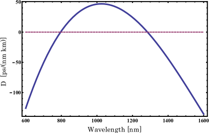
Fig. 3: The $D$ parameter for the photonic crystal fiber used in simulations from 600 nm to 1600 nm. The dashed line is at $D=0$ for reference.

Given a particular dispersion profile of a fiber and the central wavelengths at which translation will occur, the fiber can effectively translate input signals only with spectral widths smaller than the characteristic bandwidth of the BS process. As seen in equations (6) in the case of low conversion efficiency, the state is proportional to sinc$(\Delta\beta L/2)$, which defines the dispersive mismatch of the process. Figure 4 shows this sinc function for the fiber, central wavelengths, and length (20 m) used in the simulations. All fields were taken to be monochromatic, and the pumps where fixed at 808 nm and 845 nm. The “blue” signal field was varied from its central wavelength of approximately 649 nm (shown in frequency on the horizontal axis) while the “green” field was varied from its central wavelength of 673 nm to conserve the energy of the process $(\omega_{s}=\omega_{p}+\omega_{i}-\omega_{q})$. The full-width at half-maximum (FWHM) of the central sinc lobe is approximately 0.3 Trad/s. This number gives a rough estimate of the effective bandwidth of the BS process. As we will see, all else being equal, input signals that have spectral widths larger than this number do not translate as efficiently as signals that have spectral widths lower than this number.

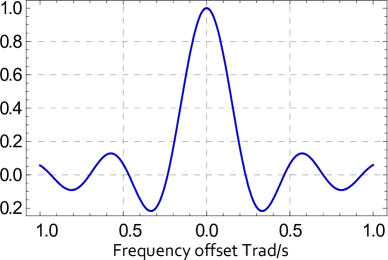
Fig. 4: Phase-matching function sinc($\Delta\beta L/2)$ for the fiber used in the simulation, where the pump wavelengths were fixed and the “green” and “blue” fields frequencies were varied in an energy-conserving manner. The horizontal axis is the “green” frequency variation from its corresponding central wavelength value of 673 nm. For this plot the fiber length is $L=20$m, and the FWHM of the function is approximately 0.3 Trad/s ($10^{12}$ rad/s).

4 Numerical results

This section details the results of simulations for several different cases, broken up into two main categories; cases that highlight properties relating to effective total translation from one signal field to another, and cases that highlight properties relating to good two-color HOM interference. For the cases in which the Green function of the process was calculated, the two pumps were identical transform-limited Gaussian-shaped fields. The pump intensity profiles had either a “long” FWHM duration of 1000 ps, making them quasi-CW for most input signal fields used, or a “short” FWHM duration of 70 ps. At the input to the fiber, the centers of the fields were placed at zero time. The central wavelengths for the pump fields $p$ and $q$ were 808 nm and 845 nm, respectively, placing them in the anomalous-dispersion region. The signals “green” $g$ and “blue” $b$ were at wavelengths 673 nm and 649 nm, respectively, placing them in the normal-dispersion region. The 845-nm and 649-nm fields had nearly equal group velocities ($\cong 2.0044\times 10^{8}$ m/s), and the 808-nm and 673-nm fields had nearly equal group velocities ($\cong 2.0049\times 10^{8}$ m/s). The nonlinear coefficient $\gamma$ was set to $100\;\textrm{W}^{-1}\textrm{km}^{-1}$ for all calculations.

The Green functions were calculated in the HG mode basis, where the input and output field amplitudes were decomposed into a common set of HG functions. The Green function for a particular case was found by sequentially setting the green or blue input field to a single Hermite-Gaussian function, solving the propagation, and projecting the output pulse onto the HG basis functions. Thereby the green function is represented in the HG mode basis. The characteristic time scale for the HG functions, which we define as the FWHM of the zeroth order HG function, used to produce the figures was found by first arbitrarily choosing a characteristic time of 40 ps, fitting the resulting absolute value of the first Schmidt mode to a Gaussian function, and calculating the Green function again using this new characteristic time. This time-scale choice for defining an “optimal HG basis” produced Green function matrices that were the least complex, some of which were nearly diagonal, and therefore the simplest to understand. The HG basis set was centered in time at the peak of the pump and signal inputs.

Parameter studies were also carried out in which the two pump pulses’ intensity durations were set at 1000 and 70 ps, and the input signal field durations were varied. Either the translation efficiency or HOM interference properties were documented, depending on the main category of the case.

There are a few ways in which to gauge the accuracy of the numerical solutions. While not explicitly built into the calculations, for all calculations the sum of the green and blue pulse energies (calculated in the frequency domain) were found to be conserved, in accordance with the Manley-Rowe relation [22] for the BS process. Also, there are unitary conditions on the Green functions that govern the process, given by (11). Although checking these conditions is significantly more expensive computationally than verifying the Manley-Rowe relations, and therefore is not feasible for studies requiring large numbers of cases like the below-mentioned parameter studies, this check was carried out for several representative cases for such studies. The Green functions were then checked against (11), and in these cases were found to agree well. Finally, the appropriate number of steps were taken for each calculation so that the solutions converged and were not meaningfully dependent on the exact number of steps.

4.1 Frequency translation, long pulse

Figures 5, 6, and 7 detail the case where the pump pulses were 1000 ps long and had peak powers of 400 mW. It was found by trial and error that translation occurred efficiently at a fiber length of 20 m for pumps with peak powers around 400 mW. It was found that the characteristic time of the optimal HG basis was $\approx 243$ ps. Figure 5(a) shows the absolute value of the $V$ matrix, as defined in (13), from an SVD of the $G_{gb}$ Green function. This Green function corresponds to the case of translation from the green mode to the blue mode. As discussed previously, the columns of the $V$ matrix represent the input Schmidt modes, so in this case the $V$ matrix represents the input signal field. That is,

$$V_{n}(\omega)=\sum_{j}c_{j}^{n}\psi_{j}(\omega).$$ (31)

The horizontal axis is the Schmidt mode number $n$, where order was determined by the magnitude of the corresponding singular value $\rho$, largest to smallest, for the first 25 Schmidt modes. The vertical axis is the HG mode number $j$ of the Schmidt modes using the same HG basis used to find the Green function. The plotted quantity is $|c_{j}^{n}|$. For example, the first Schmidt mode of the $V$ matrix is mostly composed of the first HG function and almost completely described by the first four HG functions. Thus we can conclude that the temporal duration of the first Schmidt mode is close to the characteristic time of the optimal HG basis, 243 ps.

Fig. 5: Singular values, $V$ matrix (columns of which are coefficients in the HG basis for individual Schmidt modes), and $w$ matrix of $G_{gb}$ Green function relating to the case with long pumps (1000 ps) having peak powers of 400 mW and a fiber length of 20 m. (a) Absolute value of the $V$ matrix (input Schmidt modes). (b) Absolute value of the $w$ matrix (output Schmidt modes). (c) Squared singular values $\rho^{2}$ (red) and $\tau^{2}$ (blue) indexed by the corresponding Schmidt mode number.

The output Schmidt modes, which physically are the results of propagating each corresponding input Schmidt mode through the QFT process in the fiber, are described by the $w$ matrix. The absolute value of this matrix, the column vectors of which correspond to output in the blue mode, is shown in Fig. 5(b). The axes are the same as those in part (a). Interestingly, the $V$ and $w$ matrices are qualitatively similar, although the $w$ matrix Schmidt modes tend to be dominated by either even or odd HG functions whereas the $V$ matrix Schmidt modes are composed of a more or less equal number of even and odd HG functions.

The black circles of the red line in Fig. 5(c) are the squared singular values $\rho^{2}$ of the $G_{gb}$ Green function for this case. The circles of the blue line correspond to the squared singular values $\tau^{2}$ of the $G_{gg}$ Green function. The $\rho^{2}$ describe the translation efficiencies of the input green Schmidt modes to the output blue Schmidt modes, whereas the $\tau^{2}$ describe the “non-translation” efficiencies of the input green Schmidt modes to the output green Schmidt modes . This corresponds to the transmission and possible reshaping of the green mode. For the Manley-Rowe relations to be satisfied, the square of these singular values must add to one, which they do numerically in this case (as well as in all other cases) to one part in one thousand. As is evident from the figure, many of the modes translate efficiently with the first several having efficiencies of over 90 percent. We call this configuration “non-discriminatory” in the sense that it effectively translates many different dissimilar modes efficiently.

Figure 6 shows the translation efficiency as a function of length long the fiber for the first three green input Schmidt modes. Here translation efficiency is defined as the number of photons in the blue mode divided by the initial number of photons in the green mode. Note that there were initially no photons in the blue mode. The red, green, and blue lines correspond to the first, second, and third Schmidt modes, respectively. The efficiency for these modes is very sinusoidal, almost as if the signals were monochromatic and described by (5) and (6).

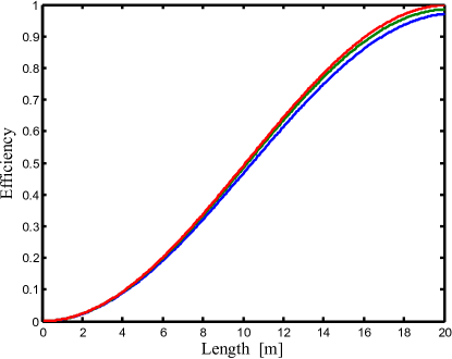
Fig. 6: Translation efficiency as a function of length along the fiber relating to the case with long pumps (1000 ps) having peak powers of 400 mW. The red, green, and blue lines relate to the first, second, and third green Schmidt modes, respectively.

Figure 7 shows the absolute amplitudes and phases in both time and frequency of the first three input Schmidt modes (relating to the $V$ matrix) of the green (673 nm) mode. The input amplitudes of the pump fields are also shown as a black dashed line. As could be guessed from Fig. 5(a), the modes look very much like HG functions, although there is some asymmetry and delay in both time and frequency. These effects are likely the results of pump evolution, which includes convection, dispersion and CPM. Figure 7(a) shows that first few Schmidt modes are much narrower in time than the pump fields. Looking at Fig. 7(b), which shows the phases in time, all the input Schmidt modes, disregarding the $\pi$ phase jumps, are distinctly parabolic with positive curvature. For the phase convention we use, this shape implies the Schmidt modes at the fiber’s input are down-chirped (frequency decreases in time), meaning that when they propagate through the medium, which for the signals is normally-dispersive, they will temporally compress. That is, they are dispersion pre-compensated. CPM also chirps the signals in the same way as linear dispersion. Figure 7(c) shows that the pump fields are nearly monochromatic as compared to the Schmidt modes, although all modes are well within the translation phase-matching bandwidth of the fiber.

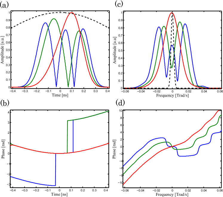
Fig. 7: Amplitude and phase in both frequency and time of the green 673-nm input Schmidt modes relating to the case with long pumps (1000 ps) having peak powers of 400 mW. The red, green, and blue lines relate to the first, second, and third Schmidt modes, respectively. Note: Trad/s indicates $10^{12}$ rad/s.

4.2 Frequency translation, short pulse

Figures 8, 9, and 10 detail the case where the pump pulses were 70 ps long and had peak powers of 400 mW. The goal in studying this case in relation to the former case is to highlight how using temporally shorter and spectrally broader pump pulses impacts the translation properties of the process. It was found that the characteristic time of the optimal HG basis for this case was $\approx 43$ ps. Figure 8(a) shows the absolute value of the $V$ matrix (input green Schmidt modes) from the SVD of the $G_{gb}$ Green function, while Fig. 8(b) shows the absolute value of the $w$ matrix (output Schmidt modes). The horizontal and vertical axes have the same meaning as they did in the previous case.

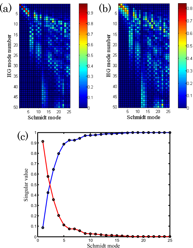
Fig. 8: Singular values, $V$ matrix, and $w$ matrix of $G_{gb}$ Green function relating to the case with short pumps (70 ps) having peak powers of 400 mW. (a) Absolute value of the $V$ matrix. (b) Absolute value of the $w$ matrix. (c) Squared singular values $\rho^{2}$ (red) and $\tau^{2}$ (blue) index by the corresponding Schmidt mode number.

While the absolute values of the $V$ and $w$ matrices are qualitatively similar, they are significantly different from their counterparts of the previous case. While they start out for low mode order approximately diagonal, like in the previous case, the Schmidt modes quickly become seemingly random and unordered. This is likely due to these Schmidt modes’ singular values [the squared value of the singular values are shown on the red line of Fig. 8(c)], which quickly drop to almost zero, signifying that almost no translation occurred. Since there is an infinite number of Schmidt modes with singular values near zero (practically any random combination of HG modes generally leads to a low singular value), even Schmidt modes of relatively low Schmidt mode number that have singular values close to zero can look random (non-uniquely defined) in the HG basis. Since in this case only the first few modes translate with significant efficiency, we call this configuration “discriminatory” in the sense that only a few closely related modes effectively translate.

Figure 9 shows the translation efficiency as a function of length along the fiber for the first three input green Schmidt modes in the short-pumps case. The red, green, and blue lines correspond to the first, second, and third Schmidt modes, respectively. Unlike the former long-pumps case, the efficiency curves of the modes are drastically different, relating to the fact that their singular values are quite different.

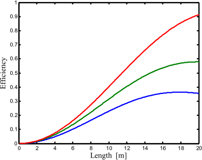
Fig. 9: Translation efficiency as a function of length along the fiber relating to the case with short pumps (70 ps) having peak powers of 400 mW. The red, green, and blue lines relate to the first, second, and third green Schmidt modes, respectively.

Figure 10 shows the absolute amplitudes and phase in both time and frequency of the first three green 673 nm input Schmidt modes (relating to the $V$ matrix). The input amplitudes of the pump fields are also shown as a black dashed line. Qualitatively, the amplitudes for this case are similar to the amplitudes in the former case; although asymmetric, they are roughly HG-like. Quantitatively, these amplitudes are much broader spectrally than in the former case. The phases in time are essentially parabolas with positive curvature much larger than that of the previous case, as expected because the bandwidths are much larger.

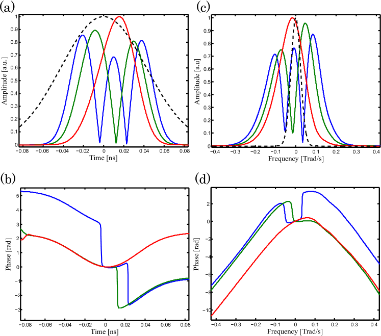
Fig. 10: Amplitude and phase in both frequency and time of the green 673-nm input Schmidt modes relating to the case with short pumps (70 ps) having peak powers of 400 mW.

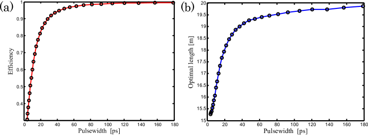
Fig. 11: Parameter study relating to frequency translation in the case with long pumps (1000 ps) having peak powers of 400 mW and fiber length 20 m. (a) The maximal translation efficiency achieved in the fiber as a function of signal pulse width. (b) The length at which the maximal translation efficiency is achieved as a function of signal pulse width.

Figure 11 shows a parameter study where the pump pulses are identical Gaussians with temporal FWHM durations of 1000 ps and peak powers of 400 mW. In Fig. 11 (a), the maximal translation efficiency achieved along the fiber is plotted as a function of input signal pulse FWHM duration. For relatively “long” pulses in low hundreds of picoseconds, the translation efficiency is quite high due to the near-CW nature of the pump and the width of the translation bandwidth. As the pulses become shorter, particularly around 43 ps, which corresponds to a spectral bandwidth of $92$ Grad/s, the pulse spectral width begins to match that of the translation phase-matching bandwidth. Therefore, this dramatic drop in efficiency is likely caused by the signal spectral bandwidth being too large for the BS process to accommodate. In Fig. 11(b), the length at which the maximal translation occurs is plotted as a function of input signal duration. The curve has the same qualitative shape as the curve in part (a); for short signal durations, the length at which maximal translation occurs is shorter than that of signals with long durations. This likely is due to the fact that short pulses have large spectral bandwidths, which because of CPM from the pumps, become even more spectrally broad as they evolve, making them in harder to translate. Hence the best translation occurs for these signals when they haven’t evolved much. Signals with long duration and small spectral width do not spread out in frequency as much as the short signals do, so they are less limited by the magnitude of the translation bandwidth and achieve good translation along the entire fiber.

Figure 12 show a parameter study where the pump pulses are identical Gaussians with temporal FWHM durations of 70 ps and peak powers of 400 mW. The efficiency, shown in part (a), for short signal inputs behaves similarly to the previous long-pumps cases; around 20 ps the efficiency drops sharply due to the signal having larger translation phase-matching bandwidth than the fiber. Unlike the previous case, the efficiency reaches a maximum around 35 ps and slowly declines for wider input signal widths. Relatedly, it is at about this signal width that the length at which the maximal efficiency occurs, shown in part (b), is equal to the length of the fiber, suggesting that the translation efficiency would be higher for a longer fiber or higher fiber for these signal widths. As the signal width becomes equal and then greater to the pumps widths there are two main elements affecting the efficiency; the lack of power/fiber length and the fact that the pump pulses no longer fully encompass the signal pulse in time. Both of these lead to lower translation efficiency. But it is important to note that for some signal width range, from about 25 ps to 60 ps, reasonably good translation efficiency will occur for short pump pulses with reasonable parameters such as peak pump powers of 400 mW and a fiber length of 20 m.

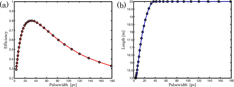
Fig. 12: Parametric study relating to the case with short pumps (70 ps) having peak powers of 400 mW and fiber length 20 m. (a) The maximal translation efficiency achieved in the fiber as a function of signal pulse width. (b) The length at which the maximal translation efficiency is achieved as a function of signal pulse width.

4.3 HOM interference, long pulse

Figures 13, 14, and 15 detail the case where the pump pulses were 1000 ps long and had peak powers of 200 mW. This configuration was designed to exhibit good two-color HOM interference by lowering the pumps’ peak power so as to lessen the translation efficiency, since the HOM interference effect is optimal when 50 percent, not 100 percent, translation occurs. It was found that the characteristic time of the optimal HG basis was $\approx 146$ ps. Figure 13(a) shows the absolute value of the $V$ matrix, as defined in (13), from an SVD of the $G_{gb}$ Green function. This Green function corresponds to the case of translation from the green mode to the blue mode. Figure 13(b) shows the absolute value of the $w$ matrix. The horizontal and vertical axes are the same as they were the previous cases. Surprisingly, both the $V$ and $w$ matrices are nearly diagonal, meaning that the input Schmidt mode set and the HG basis functions are nearly identical. In Appendix B we present a theoretical model explaining this result. The long pump pulse of 1000 ps enables many modes to be translated with nearly similar efficiencies, as can be seen from 13(c). For this reason we describe this case as “non-discriminatory” with respect to its two-color HOM interference properties, since many different types of modes lead to good HOM interference.

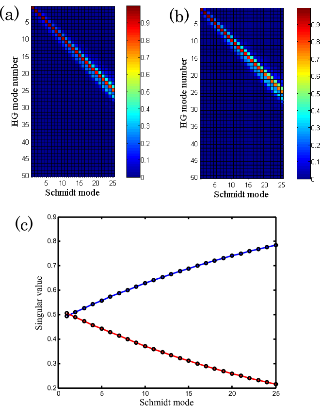
Fig. 13: Singular values, $V$ matrix, and $w$ matrix of $G_{gb}$ Green function relating to the case with long pumps (1000 ps) having peak powers of 200 mW optimized for good HOM interference. (a) Absolute value of the $V$ matrix. (b) Absolute value of the $w$ matrix. (c) Squared singular values $\rho^{2}$ (red) and $\tau^{2}$ (blue) index by the corresponding Schmidt mode number.

Figure 14 shows the HOM singular values, as defined by (17), as a function of Schmidt mode number, and the value of $P_{11}$ for the first three input Schmidt modes as a function of fiber length. We emphasize that a value $P_{11}$=0 means that two green or two blue photons exit the fiber, but never one green and one blue. This is the HOM interference effect as it applies to interference of photons of different colors [10]. Figure 14(a) shows clearly why this case is non-discriminatory in regards to its HOM interference properties; many orders of Schmidt modes exhibit HOM singular values near one.

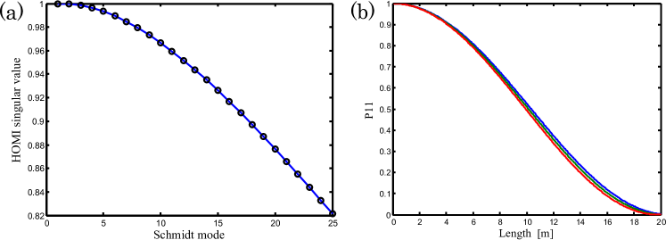
Fig. 14: HOM singular values $2\rho_{n}\tau_{n}$ and $P_{11}$ values relating to the case with long pumps (1000 ps) having peak powers of 200 mW. (a) HOM singular value index by Schmidt mode number. (b) Two-photon coincidence count probability $P_{11}$ as a function of length for the first three input Schmidt modes.The red, green, and blue lines relate to the first, second, and third Schmidt modes, respectively.

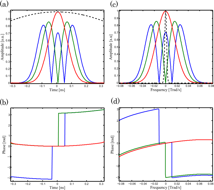
Fig. 15: Amplitude and phase in both frequency and time of the first three green 673-nm input Schmidt modes relating to the case with long pumps (1000 ps) having peak powers of 200 mW. The red, green, and blue lines relate to the first, second, and third Schmidt modes, respectively.

Figure 15 shows the absolute amplitudes and phase in both time and frequency of the first three green input Schmidt modes (relating to the $V$ matrix). The input amplitudes of the pump fields are also shown as a black dashed line. Since the $V$ matrix is nearly diagonal, the Schmidt mode amplitudes are almost quantitatively identical to the HG basis functions, which stands in contrast to the case in section 4.1 which had the same duration pulse length but twice the pump power. Similarly to the previous cases, the phase in time is parabolic with positive curvature, showing that these inputs are also down-chirped.

4.4 HOM interference, short pulse

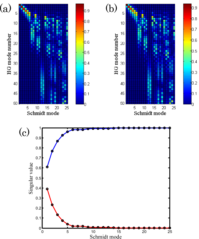
Fig. 16: Singular values, $V$ matrix, and $w$ matrix of $G_{gb}$ Green function relating to the case with short pumps (70 ps) having peak powers of 200 mW, optimized for good HOM interference. (a) Absolute value of the $V$ matrix. (b) Absolute value of the $w$ matrix. (c) Squared singular values $\rho^{2}$ (red) and $\tau^{2}$ (blue) indexed by the corresponding Schmidt mode number.

Figures 16, 17, and 18 detail the case where the pump pulses were 70 ps in duration and had peak powers of 200 mW, which is close to the optimum for good HOM interference. The goal in studying this case is to contrast it with the former case that had pumps with the same peak power but were much longer in duration. This will highlight the relative importance of having spectrally broad and temporally short pump pulses in regards to the HOM interference behavior. It was found that the optimal characteristic time of the HG basis for this case was $\approx 38$ ps. Figure 16(a) shows the absolute value of the $V$ matrix from the SVD of the $G_{gb}$ Green function, while Fig. 16(b) shows the absolute value of the $w$ matrix. The horizontal and vertical axes are the same as they were in the previous cases.

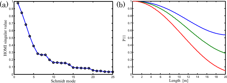
Fig. 17: HOM singular values and $P_{11}$ relating to the case with short pumps (70 ps) having peak powers of 200 mW. (a) HOM singular values indexed by Schmidt mode number. (b) Two-photon coincidence count probability $P_{11}$ values as a function of length along the fiber for the first three input Schmidt modes. The red, green, and blue lines relate to the first, second, and third Schmidt modes, respectively.

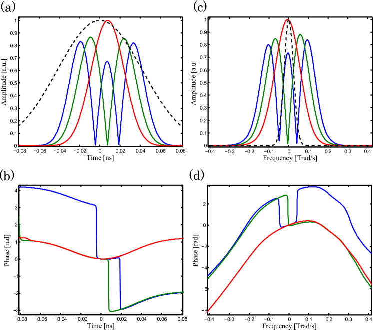
Fig. 18: Amplitude and phase in both frequency and time of the green 673-nm input Schmidt modes relating to the case with short pumps (70 ps) having peak powers of 200 mW. The red, green, and blue lines relate to the first, second, and third Schmidt modes, respectively.

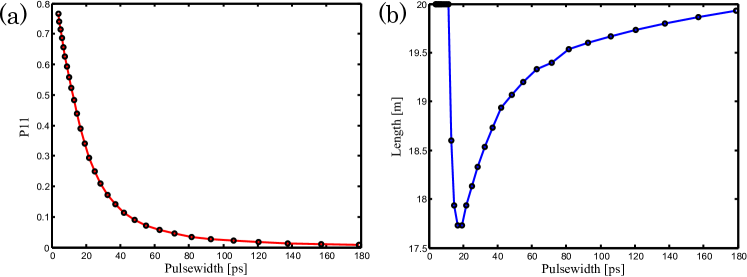
Fig. 19: Parametric study relating to the case with long pumps (1000 ps) having peak powers of 200 mW. (a) The minimal $P_{11}$ value achieved in the fiber as a function of signal pulse duration. (b) The length at which the minimal $P_{11}$ value is achieved as a function of signal pulse duration.

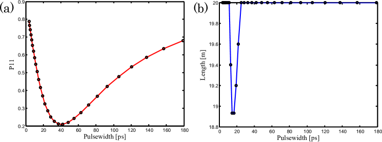
Fig. 20: Parametric study relating to the case with short pumps (70 ps) having peak powers of 200 mW. (a) The minimal $P_{11}$ value achieved in the fiber as a function of signal pulse duration. (b) The length at which the minimal $P_{11}$ value is achieved as a function of signal pulse duration.

Like the previous cases, both the $w$ and $V$ matrices are nearly diagonal for low Schmidt mode number, but unlike the previous case, they quickly become seemingly random combinations of HG functions for higher-order Schmidt modes. The reason for this is the same as it was in the other case having short pump pulses; there are many Schmidt modes that have low singular values, and practically any combination of higher-order HG functions will have a low, but non-zero singular value. As shown in Fig. 16(c), only the first few Schmidt modes have a singular value meaningfully above zero and will therefore have a more ordered mode structure.

Figure 17 plots the HOM singular values, as defined by (17), as a function of Schmidt mode and the value of the two-photon coincidence count probability $P_{11}$ for the first three input Schmidt modes as a function of fiber length. Figure 17(a) shows that, in contrast to the previous case, the HOM singular values decrease rapidly with Schmidt mode number, making this case highly “discriminatory” in regards to its HOM interference properties; only a few Schmidt modes exhibit HOM singular values significantly above zero.

Figure 18 shows the absolute amplitudes and phase in both time and frequency of the first three green input Schmidt modes (relating to the $V$ matrix). The input amplitudes of the pump fields are also shown as a black dashed line. Similarly to the previous case, these first few Schmidt modes are qualitatively similar to the HG basis functions, although they exhibit more asymmetry relative to their width than do the Schmidt modes in the previous case. As can be seen in Fig. 18 (c), the frequency amplitudes have widths that are comparable to (and, for the second and third mode, somewhat larger than) the translation bandwidth, which contributes to the fact that the higher-order modes experience a low translation efficiency. The phase plots are similar to what they were in the previous cases; the phases in time are mostly parabolic with positive curvature, implying the inputs are down-chirped.

Figure 19 shows a parameter study where the pump pulses are identical Gaussians with temporal FWHM durations of 1000 ps and peak powers of 200 mW. In Fig. 11 (a), the minimal $P_{11}$ value achieved along the fiber is plotted as a function of input signal pulse FWHM duration. For short signal durations the minimum $P_{11}$ value hardly changes from 1, which is the initial value ($z=0$) of $P_{11}$ for all modes, but for long signal durations the minimum $P_{11}$ value drops to nearly zero. This is most likely due to the short signals having large spectral bandwidths and the long signals having small spectral bandwidths as compared to the translation bandwidth. This follows because pulses with large relative bandwidth experience poor translation as compared to pulses with small relative bandwidths. In Fig. 11(b), the length at which the minimal $P_{11}$ value occurs is plotted as a function of input signal duration. For short signal widths, the optimal length is the same as the fiber length. This is likely due to the difficulty translating signals with large bandwidths; it takes the entire length of the fiber to translate the small amount of the signal that is within the translation phase-matching bandwidth. This dynamic changes once the signal width is on the order of the phase-matching bandwidth, at which point the BS process is no longer limited by bandwidth but by the shape and power of the pumps, hence the longer optimal lengths for longer signal pulses.

Figure 20 shows a parameter study where the pump pulses are identical Gaussians with temporal FWHM durations of 70 ps and peak powers of 200 mW. The value of $P_{11}$, shown in part (a), for short signal inputs behaves similarly to the previous long-pumps case: a sharp increase in $P_{11}$ for very short signal widths due to the signal having larger translation phase-matching bandwidth than the fiber. Unlike the previous case, $P_{11}$ reaches a minimum around 40 ps and begins to slowly increase for wider input signal widths. The increase for wider signal widths is likely due to signals beginning or evolving to be wider than the pumps, so that only part of the signals wavepacket could be translated. The length at which the minimum $P_{11}$ occurs is shown in part (b). This is a qualitatively similar result to the previous long-pumps cases. For short signals the optimal length is equal to the length of fiber (fixed at 20 m), due to the excessive bandwidth of the signal in relation to the phase-matching bandwidth. But when the signal durations are of the same order as the pumps, the optimal length is not as constrained by the phase-matching bandwidth in the same manner, and becomes somewhat shorter than the length of the fiber. But when the signals become as long as or longer than the pump, the overlap between all the fields in time significantly decreases, leading to less translation and raising the value of $P_{11}$. In this regime the fiber length also limits the translation, hence the reason the optimal length is equal to the length of the fiber. This suggests that were the fiber longer the value of $P_{11}$ would be lower, which indeed is the case.

5 Analytic derivation of Schmidt modes

In order to gain further insight into the numerical simulations presented above, we developed an analytical perturbative solution, valid for not-too-high conversion efficiencies. The main insights provided by this solution are: (1) The Schmidt modes are found, to good approximation, to equal HG functions in this regime. (2) The origin of the input Schmidt mode temporal delays seen in Figs. 15 and 18 can be understood as arising from differences of group velocities and the requirement for maximal interaction with the pump pulses in the fiber.

The detailed derivation is given in Appendix B, the results of which are summarized here. Equations (13)–(16) show how, in general, to express the backward Green functions as sums of products of the input Schmidt modes $V_{n}$ and $W_{n}$, the output modes $v_{n}$ and $w_{n}$, and the Schmidt coefficients $\rho_{n}$ and $\tau_{n}=(1-\rho_{n}^{2})^{1/2}$. Furthermore, the diagonal Green functions $G_{gg}$ and $G_{bb}$ can be deduced from the off-diagonal Green functions $G_{gb}$ and $G_{bg}$ (and vice versa). In Appendix B we rewrite the third and fourth lines of (25) in a frame moving with the average group speed of the signals. We include the effects of signal convection and second-order dispersion, but do not include the effects of time-dependent cross-phase modulation, which were discussed qualitatively after Fig. 7. In this frame the dispersion relations for the green and blue signal fields $k_{g}(\omega_{g})=\beta_{1}\omega_{g}+\beta_{2}\omega_{g}^{2}/2$ and $k_{b}(\omega_{b})=-\beta_{1}\omega_{b}+\beta_{2}\omega_{b}^{2}/2$ give the associated wavenumbers, correct to second order in frequency difference. In our simulations $\beta_{1}$ is negative, so the green mode is faster than the blue mode. For the parameters in our simulations, the temporal walk-off of pulses is significant, but pulse broadening by linear group-velocity dispersion is negligible. Therefore, we set $\beta_{2}=0$ here for the simplest analytical solution. We assume the pumps have identical temporal intensity profiles, proportional to $\exp(-t^{2}/2\sigma^{2})$, where $\sigma$ is a width parameter. We then find that the perturbative solution for the signals (to first order in the coupling parameter $\gamma$) involves Green functions that can be expressed in SVD form, as are those in (13)–(16). In this perturbation theory the Schmidt modes are independent of the coupling parameter $\gamma$ and pump peak intensities, but of course this will break down at higher values of $\gamma$ or pump peak intensities. Notably, we find that the Schmidt modes are given by HG functions in this regime. The explicit forms of the input green and blue Schmidt modes are, respectively:

$$V(\omega_{g}) = t_{0}^{1/2}\psi_{n}(t_{0}\omega_{g})\exp(+i\omega_{g}\beta_{1}L/2),$$ (32)

$$W(\omega_{b}) = t_{0}^{1/2}\psi_{n}(t_{0}\omega_{b})\exp(-i\omega_{b}\beta_{1}L/2),$$ (33)

where the $\psi_{n}(t_{0}\omega_{g})$ are the HG functions defined in (26), and the temporal scale factor is $t_{0}=\left({0.621\sigma\beta_{1}L}\right)^{1/2}$. Likewise, the output green and blue Schmidt modes are, respectively:

$$v(\omega_{g}) = t_{0}^{1/2}\psi_{n}(t_{0}\omega_{g})\exp(-i\omega_{g}\beta_{1}L/2),$$ (34)

$$w(\omega_{b}) = t_{0}^{1/2}\psi_{n}(t_{0}\omega_{b})\exp(+i\omega_{b}\beta_{1}L/2).$$ (35)

Note that the spectral phases in these mode solutions correspond to temporal delays or advances, which in this simple model result in both green and blue modes maximally overlapping with the pump pulses at the midpoint ($z=L/2$) of the medium. In our simulations $\beta_{1}$ is negative, so the green input mode is delayed and the blue input mode is advanced (although note that in our simulations the two pumps walk off from each other, which is not the case for the analytic solution given here).

Using the same parameters as in the numerical simulations leading to Figs. 15 and 18, the approximate input Schmidt modes for the blue signal are plotted as functions of time and frequency in Figs. 21 and 22. (Note that the time-domain modes are also described by HG functions.) For conversion efficiencies up to 50%, the approximate analytical solutions predict the modes’ widths accurately, and their delays or advances qualitatively. For higher conversion efficiencies, accurate analytical solutions are not yet known. Clearly, the perturbative solutions will not hold for conversion efficiencies approaching 100%, as we see significant alterations of the modes in Figs. 7 and 10.

   

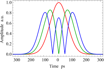
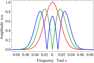
Fig. 21: Approximate Schmidt modes for the faster signal plotted as functions of time and frequency, for long pump pulses. The red, green, and blue lines denote the first, second and third input Schmidt modes, respectively.

   

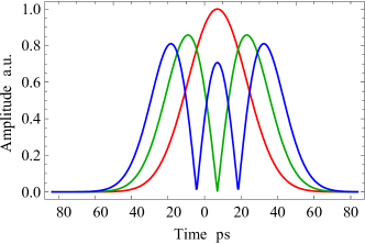
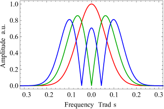
Fig. 22: Approximate Schmidt modes for the faster signal plotted as functions of time and frequency, for short pump pulses. The red, green, and blue lines denote the first, second and third input Schmidt modes, respectively.

6 Discussion and conclusions

In this paper we studied quantum frequency translation (QFT) by the four-wave mixing interaction of Bragg scattering (BS) using a realistic numerical model of photonic crystal fiber and an analytical approximate solution valid for low conversion efficiency. Because BS implements a quantum operator transformation analogous to that of an ordinary beam splitter (mode coupler), it is noiseless (background free) [3]. Furthermore, the beam-splitter nature of BS leads to linear-optical quantum operations between weak light pulses of different central frequencies, in particular two-photon Hong-Ou-Mandel (HOM) interference [10]. The main questions addressed were: (1) Under what conditions does high-efficiency QFT take place? (2) Under what conditions does high-efficiency HOM interference take place? (3) Given the shapes of the pump pulses, how can one design ideal signal pulse shapes to optimize the above-mentioned processes? (4) How are these ideal signal shapes affected by the level of the conversion efficiency for the QFT? That is, are the ideal shapes invariants for a given pump shape, or do they evolve differently at higher conversion efficiency than at low conversion efficiency?

Our modeling included realistic input pump and signal fields and effects such as convection, dispersion, self-phase modulation and cross-phase modulation. This work extends previous theoretical and numerical work [3, 10] on these subjects not only through explicitly modeling of specific cases (specific input signal wavepackets), but more generally through the determination of the Green function that governs the BS process for an entire range of input signal wave packets. Knowing the Green function for a process enables the calculation of the signal input and output Schmidt modes and corresponding singular values (generalizations of eigenmodes and eigenvalues, respectively), found by the singular value decomposition of the Green function. Knowledge of the Schmidt modes and their associated singular values enables the calculation of the effect of the BS process on the input signals without the need to further solve the pulse propagation equations. Most importantly for single-photon inputs, this includes the frequency translation and two-color two-photon interference effects. It also allows for the optimization of these effects.

In particular, conditions for achieving high translation efficiency of input signal wave packets with Gaussian pumps with both long (1000 ps) and short (70 ps) durations at a modest peak power of 400 mW were discovered by finding the Green function, and then Schmidt modes, of the process. These two cases represent the quasi-CW regime and pulsed regime, respectively, in regards to the translation phase-matching bandwidth of the process. The long-pumps case was found to be “non-discriminatory,” where many Schmidt modes were translated with high efficiency. Therefore, this configuration of fiber and pumps would be useful for effective translation of many different input signal wave packets or in the case where an input packet is a superposition of the high-efficiency ones. In contrast, the short-pump case was found to be “discriminatory,” where only the first few Schmidt modes experienced significant translation.

Configurations of the discriminatory type would be most suited to applications where it is desirable for only a few types of wave packets (ideally only one) to experience significant translation, such as in a temporal-mode-selective add/drop filter [16, 17]. Recently it was proposed that such a filter, or “pulse gate” can be implemented using frequency upconversion by sum-frequency generation in an optical crystal driven by a single strong pump pulse [15]. This process is analogous to the BS process studied here, with a major difference being that in upconversion the two signal fields being connected by frequency translation must be separated by an amount equal to the pump frequency. This limits the process to large frequency separations. The numerical scheme developed here is well suited for modeling such a process.

To gain insight into the FWM Bragg scattering process, we developed an analytical perturbation solution. We find that for low efficiency QFT the Schmidt modes are well approximated by a set of orthogonal Hermite-Gaussian functions with characteristic temporal widths determined simply by group-velocity differences and the spectral width of the pumps. Nevertheless, we emphasize that the HG modes become strongly altered for high conversion, in apparent contradiction to what is argued in [15].

Also studied were the conditions for achieving a highly visible two-color photon interference. We studied two pump configurations having long (1000 ps) and short (70 ps) durations and a peak power (200 mW) close to the optimum value for a 20-m-long fiber. Similar to the high-efficiency translation cases, the long-pump case was “non-discriminatory” and the short-pump cases was “discriminatory” in regards to high visibility of the two-color photon interference effect. We verified numerically that for the long-pumps configuration up to about 50 percent conversion efficiency, both the input and output Schmidt mode sets are very well approximated by orthogonal Hermite–Gauss (HG) function sets. For the short-pumps configuration, the HG functions are reasonable approximations. The approximate theory on which the HG functions are based allows one to predict the Schmidt-mode widths and singular values as functions of the physical parameters.

In conclusion, QFT by FWM Bragg scattering appears to be a powerful and robust technique for linearly interacting two quantum fields of distinct frequencies. Besides offering the ability to change the colors of single photons, it may offer other useful abilities in quantum information science, such as linear-optical quantum computing “over the rainbow” of optical and near-IR frequencies.

Appendix A: probabilities $P_{20}$ and $P_{02}$

The probability for the occurrence of the $|2,0\rangle$ and $|0,2\rangle$ states requires care to derive due to the possibility that degenerate photons would be created in the green and blue frequency regions. In this case the primed variables attached to the operators cannot be taken over to their unprimed counterparts (as $\omega_{b}^{{}^{\prime}}$ to $\omega_{b}$ was for example). This ambiguity can be avoided by calculating $P_{20}$ directly as the product of the appropriate bra and ket vectors (similarly for $P_{02}$). From (20) the term corresponding to the creation of two green photons leads to an expression for $P_{20}$ of

$$\begin{split}P_{20}&=\langle\psi_{20}||\psi_{20}\rangle=\langle vac|\left(\int\int d\bar{\omega}_{g}d\bar{\omega}_{g}^{{}^{\prime}}a_{g}(\bar{\omega}_{g})a_{g}(\bar{\omega}_{g}^{{}^{\prime}})A_{gg}^{*}(L,\bar{\omega}_{g})A_{gb}^{*}(L,\bar{\omega}_{g}^{{}^{\prime}})\right)\\ &\times\left(\int\int d\omega_{g}d\omega_{g}^{{}^{\prime}}a_{g}^{\dagger}(\omega_{g})a_{g}^{\dagger}(\omega_{g}^{{}^{\prime}})A_{gg}(L,\omega_{g})A_{gb}(L,\omega_{g}^{{}^{\prime}})\right)|vac\rangle\\ &=\langle vac|\int\int\int\int d\bar{\omega}_{g}d\bar{\omega}_{g}^{{}^{\prime}}d\omega_{g}d\omega_{g}^{{}^{\prime}}A_{gg}^{*}(L,\bar{\omega}_{g})A_{gb}^{*}(L,\bar{\omega}_{g}^{{}^{\prime}})A_{gg}(L,\omega_{g})A_{gb}(L,\omega_{g}^{{}^{\prime}})\\ &a_{g}(\bar{\omega}_{g})a_{g}(\bar{\omega}_{g}^{{}^{\prime}})a_{g}^{\dagger}(\omega_{g})a_{g}^{\dagger}(\omega_{g}^{{}^{\prime}})|vac\rangle,\\ \end{split}$$ (36)

where the variables of the conjugate wavefunction are denoted with an overhead bar. The key to evaluating this expression is to utilize the field commutation relation. In the frequency variable the commutation relation is $[a(\omega),a^{\dagger}(\omega^{{}^{\prime}})]=\delta(\omega-\omega^{{}^{\prime}})$. Hence the commutation relation to be used on the innermost operators is

$$a_{g}(\bar{\omega}_{g}^{{}^{\prime}})a_{g}^{\dagger}(\omega_{g})=\delta(\bar{\omega}_{g}^{{}^{\prime}}-\omega_{g})+a_{g}^{\dagger}(\omega_{g})a_{g}(\bar{\omega}_{g}^{{}^{\prime}}).$$ (37)

This breaks the expression into two parts, and leads to the expression, employing dummy variable notation,

$$P_{20}=\left|\int d\omega A_{gg}^{*}(L,\omega)A_{gb}(L,\omega)\right|^{2}+\int d\omega d\omega^{{}^{\prime}}|A_{gg}(L,\omega)|^{2}|A_{gb}(L,\omega^{{}^{\prime}})|^{2}.$$ (38)

The expression for $P_{02}$ is the same when $A_{gg}\rightarrow A_{bb}$ and $A_{gb}\rightarrow A_{bg}$. The two terms of (38) have distinct physical interpretations. The first term, derived in part from the delta function of (37), is essentially the overlap of the two spectral functions $A_{gg}$ and $A_{gb}$, and accounts for cases in which the two green photons are created in the same mode. This purely quantum mechanical term arises from the bosonic nature of photons, the operators of which obey the above-mentioned commutation relation. The second term accounts for the cases in which the two green fields are purely classical, as if these fields did not obey the quantum bosonic commutation relations.

Appendix B: derivation of the approximate Schmidt modes

According to (13)–(16), the (backward) constituent Green functions are determined by the input Schmidt modes $V_{n}$ and $W_{n}$, the output modes $v_{n}$ and $w_{n}$, and the Schmidt coefficients $\rho_{n}$ and $\tau_{n}=(1-\rho_{n}^{2})^{1/2}$. Furthermore, the diagonal Green functions $G_{gg}$ and $G_{bb}$ can be deduced from the off-diagonal Green functions $G_{gb}$ and $G_{bg}$ (and vice versa). In this appendix, the off-diagonal Green functions and the associated Schmidt modes will be determined approximately, for low conversion efficiencies.

The third and fourth of (24) govern the signal evolution in the time domain. In the frequency domain, the signal equations are

$$\partial_{z}A_{g}(z,\omega_{g}) = ik_{g}(\omega_{g})A_{g}(z,\omega_{g})+i\int\overline{\gamma}(z,\omega_{g}-\omega_{b})A_{b}(z,\omega_{b})d\omega_{b},$$ (39)

$$\partial_{z}A_{b}(z,\omega_{b}) = ik_{b}(\omega_{b})A_{b}(z,\omega_{b})+i\int\overline{\gamma}^{*}(z,\omega_{b}-\omega_{g})A_{g}(z,\omega_{g})d\omega_{g},$$ (40)

where $\omega_{j}$ is an envelope frequency, $k_{g}(\omega_{g})=\beta_{1}\omega_{g}+\beta_{2}\omega_{g}^{2}/2$ and $k_{b}(\omega_{b})=-\beta_{1}\omega_{b}+\beta_{2}\omega_{b}^{2}/2$ are the associated wavenumbers (correct to second order in frequency), and $\overline{\gamma}(z,\omega)$ is the Fourier transform of the coupling term $2\gamma_{K}A_{p}^{*}(z,t)A_{q}(z,t)$ divided by $2\pi$. Equations (39) and (40) are valid in a frame moving with the average group speed of the signals (so $\pm\beta_{1}$ are the relative group slownesses). They include the effects of convection and second-order dispersion, but do not include the effect of time-dependent cross-phase modulation (which chirps the signals).

Let $A_{j}(z,\omega_{j})=B_{j}(z,\omega_{j})\exp[ik_{j}(\omega_{j})z]$. Then the transformed amplitudes $B_{j}$ obey the transformed equations

$$\partial_{z}B_{g}(z,\omega_{g}) = i\int\overline{\gamma}(z,\omega_{g}-\omega_{b})\exp[ik_{b}(\omega_{b})z-ik_{g}(\omega_{g})z]B_{b}(z,\omega_{b})d\omega_{b},$$ (41)

$$\partial_{z}B_{b}(z,\omega_{b}) = i\int\overline{\gamma}^{*}(z,\omega_{b}-\omega_{g})\exp[ik_{g}(\omega_{g})z-ik_{b}(\omega_{b})z]B_{g}(z,\omega_{g})d\omega_{g}.$$ (42)

In general, the $B$-equations are no simpler than the $A$-equations, because they depend explicitly on $z$. However, in the low-conversion-efficiency regime, one can replace the mode amplitudes on the right sides by the input amplitudes. In this regime,

$$B_{g}(L,\omega_{g}) \approx B_{g}(0,\omega_{g})+i\int_{-\infty}^{\infty}\int_{0}^{L}\kappa(z,\omega_{g},\omega_{b})B_{b}(0,\omega_{b})dzd\omega_{b},$$ (43)

$$B_{b}(L,\omega_{b}) \approx B_{b}(0,\omega_{b})+i\int_{-\infty}^{\infty}\int_{0}^{L}\kappa(z,\omega_{b},\omega_{g})B_{g}(0,\omega_{g})dzd\omega_{g},$$ (44)

where $\kappa(z,\omega_{g},\omega_{b})=\overline{\gamma}(z,\omega_{g}-\omega_{b})\exp[ik_{b}(\omega_{b})z-ik_{g}(\omega_{g})z]$ is the kernel in (41). Note that $\gamma^{*}(z,\omega)=[\gamma(z,-\omega)]^{*}$, so $\kappa(z,\omega_{b},\omega_{g})=\kappa^{*}(z,\omega_{g},\omega_{b})$.

If the pumps are Gaussian in time and identical, and their relative convection (walk-off) is neglected, then $A_{p}A_{q}=p_{0}\exp(-t^{2}/\tau^{2})$, where $p_{0}$ is the peak pump power and $\tau$ is the (Gaussian) pump width. In this case,

$$\overline{\gamma}(\omega)=[\gamma p_{0}\sigma(2/\pi)^{1/2}]\exp(-\sigma^{2}\omega^{2}/2),$$ (45)

where the width parameter $\sigma=\tau/2^{1/2}$. Define the wavenumber-mismatch function $\delta(\omega_{g},\omega_{b})=k_{g}(\omega_{g})-k_{b}(\omega_{b})$. Then

$$\delta(\omega_{g},\omega_{b})=\beta_{1}(\omega_{g}+\omega_{b})+\beta_{2}(\omega_{g}^{2}-\omega_{b}^{2})/2.$$ (46)

By combining the preceding results, and using the identity $\int_{0}^{L}e^{-i\delta z}dz=Le^{-i\delta L/2}{\rm sinc}(\delta L/2)$, one finds that the integrated kernel

$$K(\omega_{g},\omega_{b}) = [\gamma p_{0}L\sigma(2/\pi)^{1/2}]\exp[-i\beta_{1}L(\omega_{g}+\omega_{b})/2-i\beta_{2}L(\omega_{g}^{2}-\omega_{b}^{2})/4]$$ (47)

$$\times\exp[-\sigma(\omega_{g}-\omega_{b})^{2}/2]{\rm sinc}[\beta_{1}L(\omega_{g}+\omega_{b})/2+\beta_{2}L(\omega_{g}^{2}-\omega_{b}^{2})/4].$$

The $\omega_{j}$ terms in the first exponential produce delays (advances) in the time domain, whereas the $\omega_{j}^{2}$ terms produce chirps in the frequency domain (convolutions in the time domain). By making the approximation ${\rm sinc}(x)\approx\exp(-cx^{2}/2)$, where $c=0.3858$, and omitting dispersion (setting $\beta_{2}=0$), which is negligible for the parameters of our simulations, one finds that

$$K(\omega_{g},\omega_{b}) \approx [\gamma p_{0}L\sigma(2/\pi)^{1/2}]\exp[-i\beta_{1}L(\omega_{g}+\omega_{b})/2]$$ (48)

$$\times\exp[-\sigma^{2}(\omega_{g}-\omega_{b})^{2}/2-\beta^{2}(\omega_{g}+\omega_{b})^{2}/2],$$

where the walk-off parameter $\beta=c^{1/2}\beta_{1}L/2$.

Because kernel (48) is a Gaussian function of frequency, it can be decomposed using the Mehler identity [33, 34]

$$\exp\biggl{[}-{(1+\mu^{2})(x^{2}+y^{2})\over 2(1-\mu^{2})}+{2\mu xy\over(1-\mu^{2})}\biggr{]}=[\pi(1-\mu^{2})]^{1/2}\sum_{n=0}^{\infty}|\mu|^{n}\psi_{n}(x)\psi_{n}(y),$$ (49)

where the Hermite-Gaussian functions $\psi_{n}$ were defined in (27). By comparing (48) and (49), one finds that $\mu=(\sigma-\beta)/(\sigma+\beta)$, $x=t_{g}\omega_{g}$ and $y=t_{b}\omega_{b}$, where $t_{g}=(2\beta\sigma)^{1/2}=t_{b}$. Hence, kernel (48) has the singular value (Schmidt) decomposition

$$K(\omega_{g},\omega_{b})=\sum_{n=0}^{\infty}\lambda_{n}\phi_{n}(\omega_{g})\phi_{n}(\omega_{b})\exp[-i\beta_{1}L(\omega_{g}+\omega_{b})/2],$$ (50)

where the Schmidt coefficients $\lambda_{n}=\gamma p_{0}L[(\sigma/\beta)(1-\mu^{2})]^{1/2}|\mu|^{n}$ and the (normalized) Schmidt modes $\phi_{n}(\omega_{j})=t_{j}^{1/2}\psi_{n}(t_{j}\omega_{j})$. The kernel is separable when $\mu=0$ ($\sigma=\beta$), in which case $\lambda_{0}=\gamma p_{0}L$ and $t_{j}=2^{1/2}\sigma=\tau$. In this case, only one mode will be partially translated; the others will be unaffected, creating a mode-selective filter, similar to that proposed in [15].

Let $H_{gb}(\omega_{g},\omega_{b})$ be the Green function that describes the effect on the output transformed amplitude $B_{g}(L,\omega_{g})$ of the input transformed amplitude $B_{b}(0,\omega_{b})$. Then (43) implies that $H_{gb}(\omega_{g},\omega_{b})=iK(\omega_{g},\omega_{b})$. The associated (forward) Green function for the original amplitudes, $A_{g}(L,\omega_{g})$ and $A_{b}(0,\omega_{b})$, is $J_{gb}(\omega_{g},\omega_{b})=H_{gb}(\omega_{g},\omega_{b})\exp(i\beta_{1}L\omega_{g})$. Hence,

$$J_{gb}(\omega_{g},\omega_{b})=i\sum_{n=0}^{\infty}\lambda_{n}\phi_{n}(\omega_{g})\phi_{n}(\omega_{b})\exp[i\beta_{1}L(\omega_{g}-\omega_{b})/2],$$ (51)

from which it follows that the output (green) and input (blue) Schmidt mode functions are given by

$$v(\omega_{g}) = \phi_{n}(\omega_{g})\exp(-i\beta_{1}L\omega_{g}/2),$$ (52)

$$W(\omega_{b}) = \phi_{n}(\omega_{b})\exp(-i\beta_{1}L\omega_{b}/2),$$ (53)

respectively. Likewise, (44) implies that the transformed Green function $H_{bg}(\omega_{b},\omega_{g})=iK^{*}(\omega_{g},\omega_{b})$, and the original Green function $J_{bg}(\omega_{b},\omega_{g})=H_{bg}(\omega_{b},\omega_{g})\exp(-i\beta_{1}L\omega_{b})$. Hence,

$$J_{bg}(\omega_{b},\omega_{g})=i\sum_{n=0}^{\infty}\lambda_{n}\phi_{n}(\omega_{b})\phi_{n}(\omega_{g})\exp[-i\beta_{1}L(\omega_{b}-\omega_{g})/2],$$ (54)

from which it follows that the output (blue) and input (green) Schmidt mode functions are given by

$$w(\omega_{b}) = \phi_{n}(\omega_{b})\exp(+i\beta_{1}L\omega_{b}/2),$$ (55)

$$V(\omega_{g}) = \phi_{n}(\omega_{g})\exp(+i\beta_{1}L\omega_{g}/2),$$ (56)

respectively. To obtain these, we needed to account for the distinction between forward and backward Green functions, and note that here we are propagating $A$, which corresponds to the quantum operator $a$, not $a^{\dagger}$. If $\beta_{1}$ is positive, the green mode is slower than the blue mode. The preceding results show that the green input is advanced and the blue input is delayed, so their collision is centered on the midpoint of the fiber. This location maximizes the distance over which the signals interact with the peaks of the pump pulses. In our simulations $\beta_{1}$ is negative, so the green input is delayed and blue input is advanced.