Stellar Mass Black Holes in Young Galaxies

Abstract

We explore the potential cumulative energy production of stellar mass black holes in early galaxies. Stellar mass black holes may accrete substantially from the higher density interstellar media of primordial galaxies, and their energy release would be distributed more uniformly over the galaxy, perhaps providing a different mode of energy feedback into young galaxies than central supermassive black holes. We construct a model for the production and growth of stellar mass black holes over the first few gigayears of a young galaxy. With the simplifying assumption of a constant density of the ISM, $n\sim 10^{4}-10^{5}$ cm^-3, we estimate the number of accreting stellar mass black holes to be $\sim 10^{6}$ and the potential energy production to be as high as $10^{61}$ergs over several billion years. For densities less than $10^{5}$ cm^-3, stellar mass black holes are unlikely to reach their Eddington limit luminosities. The framework we present could be incorporated in numerical simulations to compute the feedback from stellar-mass black holes with inhomogeneous, evolving interstellar media.

Keywords: Galaxies: evolution - Galaxies: stellar content - Stars: massive - Black hole physics - Accretion, accretion disks - Radiative transfer

1 Introduction

Most research on the early formation and growth of black holes has focused on the important issues of the growth and feedback of intermediate and supermassive black holes; relatively little attention has been paid to the effects of stellar-mass black holes and their potential energy production. Estimates of the number of stellar mass black holes presently in the Galaxy are as high as $10^{8}$ to $10^{9}$ (Agol & Kamionkowski, 2002; Chisholm et al., 2003), suggesting that the nearest is only parsecs away, but accreting feebly from the modern interstellar medium. The cumulative energy production of $10^{8}$ $10M_{\odot}$ black holes could rival that of a single central $10^{9}M_{\odot}$ black hole.

The first stars that formed were extremely low metallicity and arguably high mass (Bromm et al., 2002) Population III stars. These stars may have only produced intermediate-mass or supermassive black holes, if any, but turbulence may broaden the initial mass function so that lower mass stars and black holes form even in the first generation (Clark et al., 2011; Prieto et al., 2011). The next generation of stars, Population II, were slightly higher in metallicity and would form stellar mass black holes. This epoch might have begun at redshift in excess of 15 (Bromm & Loeb, 2006) during the era of reionization, when the interstellar medium number density, $n_{ism}$, might still be large. In the early formation of these galaxies, their interstellar medium (ISM) density was probably much higher than it is currently, perhaps $n_{ism}\sim 10^{4}$cm^-3 (Greif et al., 2008). With ISM densities this high, stellar-mass black holes could potentially accrete substantial amounts of matter over the course of the early evolution of galaxies and emit energy back into the galaxy and intergalactic medium. Since the number of stellar mass black holes could be as high as $10^{8}$, their cumulative energy production could be extremely high, given a favorable accretion and feedback rate. Since stellar mass black holes would be distributed more evenly over the galaxy than a single supermassive black hole, the energy feedback may impact the evolution of a galaxy in different ways than would a singular source. Stellar-mass black holes also deliver feedback in a different mode than supernovae, the energy of which is primarily kinetic, and, unlike supernovae, black holes persist. The rate of star formation in galaxies is about a factor of 100 less than provided by basic estimates (Kennicutt, 1998; Somerville et al., 2008). This suggests a feedback process that has not yet been identified. The process we outline here may contribute to this regulation of star formation in early galaxy evolution.

We apply the prescriptions of black hole accretion with feedback from (Milosavljević et al., 2009) and Park & Ricotti (2011) to the stellar mass black hole case to approximate the energy production in early galaxies. With these estimations, we find that the potential energy production of the stellar mass case could be on the order of $10^{60}$ ergs over $\sim 2$ Gyr. Section 2 gives an outline of our model for the birth and growth by accretion of stellar mass black holes. Section 3 addresses the rate of accretion of stellar mass black holes including the effects of radiative feedback and gives estimates of the number of black holes, their luminosity, and their cumulative energy liberated as a function of time. Section 4 discusses the possible constraints of the Eddington limit and §5 gives our conclusions.

2 Star Formation Rate and the Black Hole Birth Rate

The total number of stars born per unit time per unit galactic mass at time, $t$, is given by:

$$r_{\star}(t)=\int_{0}^{\infty}\dot{n_{\star}}(M_{MS},t)\Phi(M_{MS})dM_{MS},$$ (1)

where $\dot{n_{\star}}(M_{MS},t)$ is the rate of birth of stars per unit galactic mass at a given time with main sequence mass, $M_{MS}$, and $\Phi(M_{MS})$ is the mass function of main sequence stars with mass between $M_{MS}$ and $M_{MS}+dM_{MS}$. The observable star formation rate per unit galaxy mass, $s_{\star}$, at a given time is then given by:

$$s_{\star}(t)=\int_{0}^{\infty}\dot{n_{\star}}M_{MS}\Phi(M_{MS})dM_{MS},$$ (2)

where $s_{\star}(t)$ has units of solar masses per year per unit galaxy mass for $M_{MS}$ measured in solar masses.

Assigning a probability, $P_{BH}(M_{MS})$, that a star of main sequence mass, $M_{MS}$, forms a black hole, the black hole birth rate, $r_{BH}(t)$, and mass formation rate, $s_{BH}(t),$ per unit galaxy mass are given by:

$$r_{BH}(t)=\int_{0}^{\infty}\dot{n_{\star}}\Phi(M_{MS})P_{BH}(M_{MS})dM_{MS},$$ (3)

and

$$s_{BH}(t)=\int_{0}^{\infty}\dot{n_{\star}}\Phi(M_{MS})M_{BH,0}(M_{MS})P_{BH}(M_{MS})dM_{MS},$$ (4)

where $M_{BH,0}(M_{MS},t,Z)$ is the initial mass of the black hole that can, in principle, be a function of the main sequence mass of its progenitor, the epoch it was born, the metallicity of the progenitor star and perhaps other parameters. Black holes in binary systems have measured masses in the range 6 - 20 M_⊙ (Casares, 2006; Shaposhnikov et al., 2011). For simplicity, we will scale our results with the assumption that all black holes are born with a single mass, $M_{BH,0}=10$ M_⊙. We can then define the efficiency, $\epsilon_{BH}$, to make black holes from a generation of stars at time $t$ as:

$$\epsilon_{BH}\equiv\frac{s_{BH}(t)}{s_{\star}(t)}\backsimeq M_{BH,0}\frac{r_{BH}(t)}{s_{\star}(t)},$$ (5)

and thus,

$$r_{BH}(t)\simeq\frac{s_{\star}(t)}{M_{BH,0}}\epsilon_{BH}(t).$$ (6)

The parameter $\epsilon_{BH}$ is proportional to the fraction of all stars that are O-type stars, $f_{O\star}$, and the fraction of O-type stars that eventually turn into black holes, $f_{BH}$. This efficiency could vary with epoch and other parameters, but, again for simplicity and illustration we will take it to be constant. We adopt $\epsilon_{BH}\sim f_{O\star}f_{BH}\sim 10^{-3}$. This corresponds approximately to making black holes from stars with $M_{MS}>30$M_⊙(that is, $P_{BH}(M_{MS}$) being a step function at 30 M_⊙) for a Salpeter mass function with minimum mass of $\sim 0.1$ M_⊙. We thus find for the rate of birth of black holes per unit galaxy mass,

$$r_{BH}(t)\simeq 1\times 10^{-4}s_{\star}(t)\epsilon_{BH,-3}M_{BH,0,10}^{-1}~{}yr^{-1}$$ (7)

where $M_{BH,0,10}$ is the mass of the initial black holes in units of 10 M_⊙  $s_{\star}(t)$ is in $M_{\odot}yr^{-1}$ per unit galaxy mass and $\epsilon_{BH,-3}$ is the black hole production efficiency in units of $10^{-3}$. Below we will want to address the rate of star formation and the associated rate of production of black holes over an entire galaxy. We define $R_{BH}(t)=M_{gal}r_{BH}(t)$ and $S_{\star}(t)=M_{gal}s_{\star}(t)$ so that

$$R_{BH}(t)\simeq 1\times 10^{-4}S_{\star}(t)\epsilon_{BH,-3}M_{BH,0,10}^{-1}~{}yr^{-1}$$ (8)

where $S_{\star}(t)$ is now the star formation rate integrated over a whole galaxy, expressed in units of solar masses per year.

3 Accretion onto Stellar Mass Black Holes in Early Galaxies

After stellar-mass black holes are born, they may grow by accretion from the early, dense, ISM. This accretion will be subject to feedback effects (Alvarez et al., 2009; Milosavljević et al., 2009; Ostriker et al., 2010; Park & Ricotti, 2011) and the accretion rate will change as the black holes grow in mass. As mentioned in the Introduction, the density of the ambient ISM, $n_{ism}$, could have been much higher in early galaxies, with some estimates as high as $10^{5}cm^{-3}$ (Greif et al., 2008; Milosavljević et al., 2009; Park & Ricotti, 2011; Debuhr et al., 2010, 2011). The ambient density is, in turn, a principal factor controlling the accretion.

During the lifetime of a massive main sequence star, stellar winds will evacuate the local interstellar medium in the vicinity of the star. The progenitor star may explode rather than collapsing quietly to form a black hole. Once the progenitor reaches the end of its lifetime and forms a black hole, there will be some time, $t_{delay}$, as the ISM refills the excavated volume, the bubble “pops” or the black hole drifts from its natal site. After this delay time, the black hole begins accreting from the ambient ISM. The time span of the delay may be diminished by neighboring stars exploding as supernovae and displacing the ambient gas and dust near the vicinity of the black hole. Estimates give $t_{delay}\sim 10^{8}yr$ (Greif et al., 2008; Wise & Abel, 2008; Greif et al., 2010). The physics governing this delay time is complex, but for simplicity we will take the delay time to be constant. Over the time spans we will consider, gigayears, this may not be an important effect, but we will formally keep the term through much of the analysis.

Recent computational models have presented accretion rates and the associated energy production with radiative energy and momentum feedback for intermediate and supermassive black holes accreting in ISM with the high densities expected in young galaxies (Alvarez et al., 2009; Milosavljević et al., 2009; Ostriker et al., 2010; Park & Ricotti, 2011). The models of Park & Ricotti (2011) are especially useful for our current purpose by providing a convenient parameterization of the effects of feedback as a ratio with respect to standard Bondi/Hoyle (Bondi & Hoyle, 1944) accretion. Park & Ricotti (2011) give the accretion rate for a stationary black hole of mass $M_{BH}$ accreting from an isothermal gas of temperature $T_{ism}$ and density $\rho_{ism}$ as:

$$\dot{M}_{BH,0}=<\lambda_{rad}>_{0}\dot{M}_{B,iso,0},$$ (9)

where the radiative feedback efficiency factor, $<\lambda_{rad}>_{0}$, is the mean ratio of the actual accretion rate to the Bondi/Hoyle accretion rate for the same ambient temperature and density, and where the subscript 0 refers to the assumption that the black hole has velocity v = 0 with respect to the ambient medium. Park & Ricotti (2011) normalize their results to the Bondi/Hoyle accretion rate for a stationary black hole in an isothermal gas with sound speed $c_{s}$ that they take to be:

$$\dot{M}_{B,iso,0}=\frac{\lambda_{B}G^{2}M_{BH}^{2}m_{p}n_{ism}}{c_{s}^{3}},$$ (10)

where $\lambda_{B}$ is a coefficient of order unity. Taking $\lambda_{B}=e^{3/2}\pi=14.08$ (Milosavljević et al., 2009), Equation 10 can be written in convenient units as,

$$\dot{M}_{B,iso,0}=1.4\times 10^{-7}M_{10}^{2}n_{ism,5}T_{ism,4}^{-3/2}\rm{M_{\odot}yr^{-1}}$$ (11)

where $M_{10}$ is the black hole mass in units of 10M_⊙, $n_{ism,5}$ is the ambient particle density in units of $10^{5}$ cm^-3, and $T_{ism,4}$ is the ambient temperature in units of $10^{4}$K, were we have taken $T_{ism}=m_{p}c_{s}^{2}/k$. For a black hole moving with a velocity, v, one would have for the Bondi/Hoyle accretion rate:

$$\dot{M}_{B,iso}=\dot{M}_{B,iso,0}\frac{c_{s}^{3}}{(v^{2}+c_{s}^{2})^{3/2}}.$$ (12)

The results of Park & Ricotti (2011) can be scaled to results appropriate for a moving black hole by an appropriate scaling of the radiative feedback efficiency factor and the Bondi/Hoyle accretion rate as indicated below.

Remarkably, Park & Ricotti (2011) (see also Milosavljević et al., 2009) find that the radiative feedback efficiency parameter, $<\lambda_{rad}>_{0}$, is independent of the the accretion efficiency, $\eta$, essentially independenent of the mass of the black hole and insensitive to the ambient density. They give:

$$<\lambda_{rad}>_{0}\sim 0.04T_{ism,4}^{-5/2}\left(\frac{T_{in}}{8\times 10^{4}\rm{K}}\right)^{-4}:n_{ism}>10^{5}\rm{cm^{-3}},$$ (13)

and

$$<\lambda_{rad}>_{0}\sim 0.04T_{ism,4}^{-5/2}\left(\frac{T_{in}}{8\times 10^{4}\rm{K}}\right)^{-4}n_{ism,5}^{1/2}:n_{ism}<10^{5}\rm{cm^{-3}},$$ (14)

where $T_{in}$ is the time-averaged temperature at the accretion radius. There is an implicit weak dependence of $<\lambda_{rad}>_{0}$ on the mass of the black hole through the parameter, $T_{in}$. The average temperature in the inner HII region will be a function of the spectral index of the radiation with harder spectral indices giving smaller accretion radii and higher $T_{in}$. We are considering smaller mass black holes than did Park & Ricotti (2011) for which the disk radiation will be harder. To allow for this, we take $T_{in}$ corresponding to the hardest spectra considered by Park & Ricotti (2011), with spectral index $\alpha=0.5$ in their Figure 9 and thus $T_{in}\sim 10^{5}$K. We ignore any other scaling of $<\lambda_{rad}>_{0}$ with $M_{BH}$, although such dependence may exist. With this scaling, we have:

$$<\lambda_{rad}>_{0}\sim 0.016T_{ism,4}^{-5/2}T_{in,5}^{-4},$$ (15)

for $n_{ism}>10^{5}\rm{cm^{-3}}$, and a multiplicative factor of $n_{ism,5}^{1/2}$ for $n_{ism}<10^{5}\rm{cm^{-3}}$.

In the final version of their paper, Park & Ricotti (2011) revised Equations 13 and 14, reducing the overall efficiency from 0.04 to 0.03 and the characteristic value of $T_{in}$ to $\sim 4\times 10^{4}$ K. These changes would alter the results here by making the overall accretion efficiency greater by a factor of $\sim$ 30. Because the value of $T_{in}$ for the case we are considering is uncertain, we have preserved our normalization to $T_{in}=10^{5}$ K. Our results can be scaled to other values of $T_{in}$ in the manner we present, but our result for the luminosity from the ensemble of stellar mass black holes may be underestimated. The energy is somewhat less sensitive than the luminosity. The time, $t_{\infty}$, for a black hole to grow to infinite mass might be smaller and more comparable to the initial accretion delay time, $t_{d}$, that we have generally neglected.

For the case of a moving black hole, the velocity correction to the accretion rate as given in Equation 12 means that for given $T_{ism}$ and $c_{s}$, the accretion rate given by Park & Ricotti (2011) is too large. The actual accretion rate for a moving black hole would be less, as if the accretion were occuring at higher effective values of $T_{ism}$ and $c_{s}$. For a given $T_{ism}$, a moving black hole would accrete at a rate corresponding to a higher effective ambient temperature of a stationary black hole such that:

$$T_{ism,v=0}=T_{ism,v>0}\frac{v^{2}+c_{s}^{2}}{c_{s}^{2}},$$ (16)

where $T_{ism,v>0}$ is the actual ambient temperature and $T_{ism,v=0}$ is the ambient temperature (and corresponding sound speed) that would give the proper accretion rate in the calculations of Park & Ricotti (2011) for stationary black holes. If, for a given ambient temperature, the accretion rate for a moving black hole corresponds to accretion at effectively a higher ambient temperature for a stationary black hole, then the values of the radiative feedback parameter derived by Park & Ricotti (2011) for a given ambient temperature must also be scaled to that same, higher effective temperature or, from Equation 15:

$$<\lambda_{rad}(T_{ism},v>0)>=<\lambda_{rad}>_{0}\left(\frac{v^{2}+c_{s}^{2}}{c_{s}^{2}}\right)^{-5/2},$$ (17)

where $<\lambda_{rad}>_{0}$ is the radiative feedback efficiency parameter for the same value of $T_{ism}$, but for a stationary black hole from Park & Ricotti (2011). We can thus write for a black hole moving with a velocity, v:

$$\dot{M}_{BH}=<\lambda_{rad}(T_{ism},v>0)>\dot{M}_{B,iso}=<\lambda_{rad}>_{0}\dot{M}_{B,iso,0}\left(\frac{v^{2}+c_{s}^{2}}{c_{s}^{2}}\right)^{-4}.$$ (18)

The results of (Park & Ricotti, 2011) for a given ambient temperature are thus equivalent to those of a somewhat higher “effective” ambient temperature for a moving black hole. This correction factor is quantitatively important, but not qualitatively important for $v\lesssim c_{s}$. The steep dependence on this factor may become significant if the black holes move supersonically through the ambient medium.

With Equations 10, 18, 13 and 14, we can write:

$$\dot{M}_{BH}=FM_{BH}^{2},$$ (19)

where the factor, F, is:

$$F=<\lambda_{rad}>_{0}\left(\frac{v^{2}+c_{s}^{2}}{c_{s}^{2}}\right)^{-4}\frac{e^{3/2}\pi G^{2}m_{p}n_{ism}}{c_{s}^{3}},$$ (20)

or

$$F=2.2\times 10^{-52}\rm{g^{-1}s^{-1}}T_{ism,4}^{-4}T_{in,5}^{-4}n_{ism,5}^{3/2}\left(\frac{v^{2}+c_{s}^{2}}{c_{s}^{2}}\right)^{-4};n_{ism,5}<1,$$ (21)

with $c_{s}^{2}=kT_{ism}/m_{p}$ and the factor of $n_{ism,5}^{3/2}$ would be $n_{ism,5}$ for $n_{ism,5}>1$. The coefficient, $F$, is a function of the ambient medium, but independent of $M_{BH}$ (except for the implicit dependence through $T_{in,5}$). The solution to Equation 19 is thus:

$$M_{BH}(t)=\frac{M_{BH,0}}{\left(1-FM_{BH,0}(t-t_{acc})\right)},$$ (22)

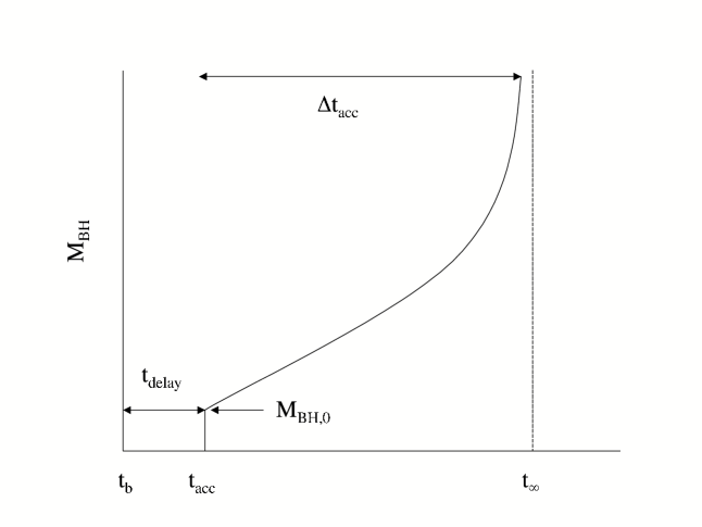
Figure 1: Schematic diagram of the growth of a black hole from a seed by feedback-limited Bondi/Hoyle accretion in an early galaxy.

where $M_{BH,0}$ is the initial mass of the black hole and $t_{acc}$ is the time when the black hole began to accrete. For a black hole born at time $t_{b}$ for which accretion was delayed by a time $t_{delay}$, then $t_{acc}=t_{b}+t_{delay}$. Figure 1 gives a schematic diagram of the growth of a black hole seed in this framework and Figure 2 gives the black hole mass as a function of time for various choices of the interstellar density, with other parameters held constant.

The timescale for a seed black hole to grow to infinite mass is given (for $n_{ism,5}<1$) by:

$$t_{\infty}=\frac{1}{FM_{BH,0}}=7.2GyrT_{ism,4}^{-4}T_{in,5}^{4}n_{ism,5}^{-3/2}\left(\frac{v^{2}+c_{s}^{2}}{c_{s,}^{2}}\right)^{4}M_{BH,0,10}^{-1}.$$ (23)

Note that this time scale increases very steeply with the velocity of the black hole. Writing the velocity correction factor as $f_{v}=(v^{2}+c_{s}^{2})/c_{s}^{2}$ and combining Equations 22 and 23, we can write:

$$M_{BH}(t)=\frac{M_{BH,0}}{\left(1-\frac{t-t_{acc}}{t_{\infty}}\right)}=\frac{M_{BH,0}}{\left(1-\frac{(t-t_{acc})n_{ism,5}^{3/2}M_{BH,0,10}}{7.2f_{v}^{4}Gyr}\right)},$$ (24)

for fiducial temperature parameters, and for $n_{ism,5}<1$. In our model, the most massive black holes will be those that began growing from seeds at a time, $t_{delay}$ after the first stellar mass black holes began to form at $t_{0}$, or $t_{acc}=t_{0}+t_{delay}$. With seed black holes of mass $M_{BH,0}=10$M_⊙, the most massive black hole will have a mass of about 14M_⊙ 2 Gy (at z   3) after the first stellar mass black holes formed and about 17M_⊙ at 3Gy. The mass would formally become infinite at 7.2 Gy for the chosen parameters, but conditions, especially $n_{ism}$, would have changed by then and the accretion might be limited by the Eddington limit. For the timescales of interest here and $n_{ism,5}<1$, this extreme growth is not of interest. We return in §4 to discuss the possible effect of growth to accretion at the Eddington limit.

We can now evaluate the number of black holes that will have formed by a certain epoch, their luminosity at that epoch, and the energy they will have emitted by that epoch.

The number of black holes of a specific mass, $M_{BH}(t)$ at a time, t, will depend on the rate at which the seed black holes were born and their accretion history. Equation 22 can be inverted to give the interval of time that a black hole of given mass has been accreting, $\Delta t_{acc}$:

$$\Delta t_{acc}=t-t_{acc}=\frac{M_{BH}(t)-M_{BH,0}}{FM_{BH,0}M_{BH}(t)}=t_{\infty}\left(1-\frac{M_{BH,0}}{M_{BH}(t)}\right).$$ (25)

Since a black hole of given seed mass was born at a time $t_{b}=t_{acc}-t_{delay}=t-\Delta t_{acc}-t_{delay}$, we can then write the time when a black hole of mass $M_{BH}(t)$ was born as:

$$t_{b}=t-t_{\infty}\left(1-\frac{M_{BH,0}}{M_{BH}(t)}\right)-t_{delay},$$ (26)

from which we can write:

$$\frac{dt_{b}}{dM_{BH}}=-\frac{1}{FM_{BH}^{2}(t)}.$$ (27)

Note the sign change here with respect to Equation 19 that results from the difference in taking the derivative with respect to t, holding $t_{b}$ constant versus taking the derivative with respect to $t_{b}$ holding the currrent epoch, t, constant. The rate at which black holes of mass $M_{BH}(t)$ at time t were born is the rate at which their seeds were born at time, $t_{b}$, which can thus be expressed as:

$$R_{BH}(t_{b})=R_{BH}(t-t_{\infty}\left(1-\frac{M_{BH,0}}{M_{BH}(t)}\right)-t_{delay}).$$ (28)

Since black holes of larger current mass were born earlier, black holes with mass between $M_{BH}$ and $M_{BH}$ + d$M_{BH}$ were born between $t_{b}$ and $t_{b}$ - d$t_{b}$. At current epoch, t, the number of black holes with mass between $M_{BH}$ and $M_{BH}$ + d$M_{BH}$ is thus given by:

$$\frac{dN_{BH}(t)}{dM_{BH}}dM_{BH}=\frac{dN_{BH}(\Delta t_{acc})}{d\Delta t_{acc}}\frac{d\Delta t_{acc}}{dM_{BH}}dM_{BH}=\frac{dN_{BH}(t_{b})}{dt_{b}}\frac{\Delta t_{acc}}{dt_{b}}\frac{dt_{b}}{dM_{BH}}dM_{BH},$$ (29)

where we have taken $\frac{dN_{BH}(\Delta t_{acc})}{d\Delta t_{acc}}=\frac{dN_{BH}(t_{b})}{dt_{b}}$. With $\frac{dN_{BH}(t_{b})}{dt_{b}}=R_{BH}(t_{b})$, $\frac{\Delta t_{acc}}{dt_{b}}=-1$, and Equation 27, we can then write:

$$\frac{dN_{BH}(t)}{dM_{BH}}dM_{BH}=R_{BH}(t_{b})\frac{dM_{BH}}{FM_{BH}(t)^{2}}.$$ (30)

The number of black holes in a galaxy with a given total star formation rate and hence total black hole formation rate born between the beginning of the epoch when stellar-mass black holes formed, $t_{0}$, and the epoch under consideration, $t$, is thus:

$$N_{BH}(t)=\int_{t_{0}}^{t}R_{BH}(t^{\prime})dt^{\prime}=\int_{M_{BH,0}}^{M_{BH,max}(t)}\frac{R_{BH}(t_{b})}{FM_{BH}(t^{\prime})^{2}}dM_{BH}+\int_{t-t_{delay}}^{t}R_{BH}(t^{\prime})dt^{\prime},$$ (31)

where $t_{b}(t^{\prime})$ is given by Equation 26 and

$$M_{BH,max}(t)=\frac{M_{BH,0}}{1-(t-t_{0}-t_{delay})/t_{\infty}},$$ (32)

is the maximum mass to which a black hole could have grown at time t, one which began accreting as soon as it could, a time $t_{delay}$ after the first stellar-mass black holes were born at $t_{0}$. The second integral over $R_{BH}$ on the right hand side accounts for the black holes that were born during the last interval, $t_{delay}$, before the epoch, t, under consideration that have not yet begun to accrete. The integral of $R_{BH}$ over the full time interval, $t_{0}$ to $t$, in Eqn 31 yields the desired result for the number of black holes (especially in the trivial case for which $R_{BH}=constant$), but the first integral on the right hand side provides the framework for evaluating the luminosity and energy production, as described below. There is no additive term over the last interval of $t_{delay}$ in the computation of luminosity and energy, since these late-born black holes are, by assumption, not yet accreting.

In principle, to evaluate the integral in Equation 31 one needs to take into account the inhomogeneity and temporal variations in the ambient quantities that determine the factor, $F$, especially $n_{ism}$ and the velocity term, $f_{v}$, and the temporal variation in the formation rate of black holes that itself is determined by variations in the star formation rate (Equation 8). When young galaxies frequently collide, the star formation rate is expected to be very bursty (Debuhr et al., 2011). To get a qualitative feel for the expectations of our framework, we will take the ambient conditions and the star formation rate to be constant in time. A representative star formation rate for a fiducial galaxy of mass $M_{gal}=4\times 10^{12}$ M_⊙ from the merging galaxy simulations of Debuhr et al. (2011) is $S_{\star}\sim 10$ M_⊙ $yr^{-1}$ and hence from Equation 8, $R_{BH}\sim 1\times 10^{-3}\epsilon_{BH,-3}M_{BH,0,10}^{-1}\left(\frac{S_{\star}}{10M_{\odot}yr^{-1}}\right)$ $yr^{-1}$. We can then write:

$$N_{BH}(t) \sim -\frac{R_{BH}}{F}\int_{M_{BH,0}}^{M_{BH,max}(t)}\frac{dM_{BH}}{M_{BH}(t)^{2}}$$ (33)

$$= R_{BH}\left(t-t_{0}\right)$$

$$\sim 1\times 10^{6}t_{Gyr}\epsilon_{BH,-3}M_{BH,0,10}^{-1}\left(\frac{S_{\star}}{10M_{\odot}yr^{-1}}\right),$$

where in the last step we have taken t to be measured in Gyr and have neglected $t_{0}$ compared to timescales of Gyr. We have taken the more cumbersome means to compute this quantity from Eqn. 31 for illustration, but note that the result is consistent with the simple integration over the rate of production of black holes. We thus estimate that over a period of 2 Gy, a galaxy like the Milky Way could have produced of order $2\times 10^{6}$ black holes that had grown from seeds of 10 M_⊙ to various masses. Figure 3 gives the number of black holes as a function of time for various choices of the initial black hole mass, $M_{BH,0}$, with other parameters held constant.

We can now use the same framework to estimate the luminosity of the ensemble of accreting stellar-mass black holes at the epoch, t. We will adopt the parameterization of Park & Ricotti (2011) with the assumption that there is sufficient angular momentum to form a disk near the black hole, so that disk-like efficiencies for turning mass accretion rates into radiated energy are applicable. For critiques of this assumption, see Ruffert & Arnett (1994); Beskin & Karpov (2005). We write for the luminosity of a single accreting black hole:

$$L(t)=\eta\dot{M}_{BH}(t)c^{2},$$ (34)

with $\eta\sim 0.1$. If a disk does not form, or forms only sporadically, the radiation efficiency would be correspondingly less than the fiducial value we assume here.

The luminosity per unit galaxy mass radiated by all black holes with mass between $M_{BH}$ and $M_{BH}+dM_{BH}$ at epoch, t, is given by:

$$\frac{dL_{tot}(t)}{dM_{BH}(t)}dM_{BH}=\frac{dN_{BH}(t)}{dM_{BH}(t)}dM_{BH}\eta c^{2}FM_{BH}^{2}(t).$$ (35)

Using Equation 29, this can be written as:

$$\frac{dL_{tot}(t)}{dM_{BH}(t)}dM_{BH}=R_{BH}(t_{b})\eta c^{2}dM_{BH}.$$ (36)

The total luminosity from all the accreting black holes born since $t_{o}$ can then be obtained by integrating over all the current masses at epoch, t, to obtain:

$$L_{tot}(t)=\int_{M_{BH,0}}^{M_{BH,max}(t)}R_{BH}(t_{b})\eta c^{2}dM_{BH}.$$ (37)

Once again, we can approximate the complex variation of the rate of production of black holes with a constant to obtain:

$$L_{tot}(t)\sim R_{BH}\eta c^{2}(M_{BH,max}(t)-M_{BH,0})=R_{BH}\eta c^{2}M_{BH,0}\left(\frac{t-t_{0}-t_{delay}}{t_{\infty}+t_{0}+t_{delay}-t}\right).$$ (38)

Neglecting $t_{0}$ and $t_{delay}$, taking $t<<t_{\infty}$, and using $N_{BH}\sim R_{BH}t$ gives a simple estimate of the luminosity of $L_{tot}\sim N_{BH}(t)\eta c^{2}M_{BH,0}/t_{\infty}$. Neglecting $t_{0}$ and $t_{delay}$ we have for the total luminosity of a galaxy of constant star formation rate:

$$L_{tot}(t)\sim\frac{8\times 10^{42}{\rm ergs^{-1}}t_{Gyr}}{1-0.14t_{Gyr}n_{ism,5}^{3/2}f_{v}^{-4}M_{BH,0,10}}\epsilon_{BH,-3}n_{ism,5}^{3/2}f_{v}^{-4}M_{BH,0,10}\left(\frac{S_{*}}{10M_{\odot}yr^{-1}}\right),$$ (39)

where we have taken the timescale $t_{\infty}$ from Equation 23 to be $7.2n_{ism,5}^{-3/2}f_{v}^{4}M_{BH,0,10}$ Gyr for fiducial temperature parameters and for $n_{ism,5}<1$. For $t\sim 2$ Gyr, the ensemble of about $10^{6}$ black holes will produce $\sim 10^{43}$ erg s^-1, as much luminosity as a modest Seyfert galaxy or a single black hole of about $10^{5}$M_⊙ accreting near the Eddington limit. For comparison, supernovae provide an input of about $L_{SN}\sim 10^{49}$ erg yr^-1 in a galaxy like the Milky Way for which the star formation rate is about 1 M_⊙ yr^-1, so a star formation rate of 10 M_⊙ yr^-1 might give $L_{SN}\sim 3\times 10^{42}$ erg s^-1. The black hole input at about 2Gy is comparable to, and might even slightly exceed the input power from supernovae. Figure 4 gives the luminosity versus time for various values of the interstellar density and Figure 5 illustrates the sensitivity of the luminosity to the velocity parameter, $f_{v}$.

The total energy liberated by the number of black holes, $N_{BH}$, accreting from $t_{o}+t_{delay}$ to $t$ is

$$E_{tot}=\int_{t_{0}+t_{delay}}^{t}L_{tot}(t^{\prime})dt^{\prime}=\int_{t_{0}+t_{delay}}^{t}\int_{M_{BH,0}}^{M_{BH,max}(t^{\prime})}R_{BH}(t_{b})\eta c^{2}dM_{BH}.$$ (40)

We will again adopt the approximation of a constant value of $R_{BH}$ to write

$$E_{tot}\sim R_{BH}\eta c^{2}\int_{t_{0}+t_{delay}}^{t}(M_{BH,max}(t^{\prime})-M_{BH,0})dt^{\prime}.$$ (41)

Invoking

$$\frac{dM_{BH,max}(t^{\prime})}{dt^{\prime}}=FM_{BH,max}^{2}(t^{\prime}),$$ (42)

we can write,

$$E_{tot}(t)=\frac{R_{BH}\eta c^{2}}{F}\int_{M_{BH,0}}^{\frac{M_{BH,0}}{1-FM_{BH,0}(t-t_{0}-t_{delay})}}\frac{M_{BH,max}-M_{BH,0}}{M_{BH,max}^{2}}dM_{BH,max},$$ (43)

which becomes

$$E_{tot}(t)=R_{BH}\eta c^{2}M_{BH,0}t_{\infty}\left\{-ln\left(1-\frac{t-t_{0}-t_{delay}}{t_{\infty}}\right)+\frac{t-t_{0}-t_{delay}}{t_{\infty}}\right\}.$$ (44)

For $t_{0}+t_{delay}<<t<<t_{\infty}$, this reduces to

$$E_{tot}\sim 2R_{BH}\eta c^{2}M_{BH,0}\left(t+\frac{1}{4}\frac{t^{2}}{t_{\infty}}\right)\sim 2L_{tot}(t)t_{\infty}\sim 2N_{BH}(t)\eta c^{2}M_{BH,0},$$ (45)

nearly independent of $t_{\infty}$. Again taking $t_{\infty}$ from Equation 23 to be $7.2n_{ism,5}^{-3/2}f_{v}^{4}M_{BH,0,10}^{-1}$ Gyr for fiducial temperatures and neglecting $t_{0}$ and $t_{delay}$ on the timescales of interest, we have:

$$E_{tot}(t) \sim 4.1\times 10^{71}\rm{ergs}~{}R_{BH}n_{ism,5}^{-3/2}f_{v}^{4}$$ (46)

$$\times\left\{-ln\left(1-0.14t_{Gyr}n_{ism,5}^{3/2}f_{v}^{-4}M_{BH,0,10}\right)+0.14t_{Gyr}n_{ism,5}^{3/2}f_{v}^{-4}M_{BH,0,10}\right\}.$$

For $R_{BH}\sim 3.2\times 10^{-11}\rm{s}^{-1}\epsilon_{BH,-3}M_{BH,0,10}^{-1}\left(\frac{S_{*}}{10M_{\odot}yr^{-1}}\right)$, we have

$$E_{tot}(t) \sim 1.3\times 10^{60}\rm{ergs}~{}\epsilon_{BH,-3}M_{BH,0,10}^{-1}\left(\frac{S_{*}}{10M_{\odot}yr^{-1}}\right)n_{ism,5}^{-3/2}f_{v}^{4}$$ (47)

$$\times\ \left\{-ln\left(1-0.14t_{Gyr}n_{ism,5}^{3/2}f_{v}^{-4}M_{BH,0,10}\right)+0.14t_{Gyr}n_{ism,5}^{3/2}f_{v}^{-4}M_{BH,0,10}\right\}.$$

For $t\sim 2$ Gyr after the beginning of stellar-mass black hole formation, corresponding to a redshift of about 3, we have

$$E_{tot}(t) \sim 1.3\times 10^{61}\rm{ergs}~{}\epsilon_{BH,-3}M_{BH,0,10}\left(\frac{S_{*}}{10M_{\odot}yr^{-1}}\right)n_{ism,5}^{-3/2}f_{v}^{4}$$ (48)

$$\times\ \left\{-ln\left(1-0.28n_{ism,5}^{3/2}f_{v}^{-4}M_{BH,0,10}\right)+0.28n_{ism,5}^{3/2}f_{v}^{-4}M_{BH,0,10}\right\}.$$

For a density of $n_{ism}=10^{5}$ cm^-3, an initial black hole mass of 10 M_⊙ and taking the velocity factor, $f_{v}$ to be unity, we get an energy liberated of $E_{tot}(t)\sim 8\times 10^{60}\rm{ergs}$ by 2 Gyr. This is equivalent to $8\times 10^{9}$ supernovae liberating about $10^{51}$ ergs apiece, but the energy would be entirely in radiant, not kinetic energy, in our model. In practice, if the black holes are accreting by means of an accretion disk, as we assume, then some of the energy emitted may be in the form of jets and hence of kinetic energy. Figure 6 gives the total liberated energy versus time for various values of the interstellar density and other parameters held constant. Figure 7 gives the total energy for various choices of the velocity parameter, $f_{v}$ at a density of $n_{ism,5}=1$. Figure 8 gives the total energy as a function of the parameter, $t_{\infty}$.

4 Eddington Limit Concerns

In the previous discussion, we have assumed accretion given by the Bondi/Hoyle rate with radiation feedback. Each seed black hole will accrete more rapidly with time, and there can be an epoch when the seed black holes reach the Eddington limit (for the relevant opacity). In this case, the accretion would proceed in a different manner.

We can solve for the time at which the Eddington limit for electron scattering is reached during the Bondi accretion phase by setting the accretion luminosity for a single black hole from Equation 34 equal to the Eddington luminosity:

$$L(M_{BH}(t))=\eta FM_{BH}^{2}c^{2}=L_{Edd}=KM_{BH}$$ (49)

where $K{\approx}10^{5}$ erg s^-1 g^-1. We thus have for the black hole mass at the Eddington limit, $M_{BH,Edd}$,

$$M_{BH,Edd}=\frac{K}{\eta Fc^{2}}\sim 250~{}M_{\odot}\ n_{ism,5}^{-3/2}f_{v}^{4},$$ (50)

for fiducial values of temperature parameters in Equation 21. The time when the first seed reaches the Eddington limit is obtained by equating $M_{BH,Edd}$ with $M_{BH,max}$ from Equation 32, neglecting the delay time, or,

$$M_{BH,Edd}=\frac{K}{\eta Fc^{2}}=M_{BH,max}=\frac{M_{BH,0}}{1-FM_{BH,0}(t_{Edd}-t_{0})},$$ (51)

or,

$$t_{Edd}-t_{0}=\frac{K-\eta Fc^{2}M_{BH,0}}{KFM_{BH,0}}\sim t_{\infty},$$ (52)

where in the final step we have neglected the second term in the numerator that is numerically small compared to $K$. Thus, formally we would have for $M_{BH}<\frac{K}{{\eta}Fc^{2}}$:

$$\dot{M}_{BH} = FM_{BH}^{2}$$

$$M_{BH} = \frac{M_{BH,0}}{1-F(t-t_{acc})M_{BH,0}}$$

$$L(t) = {\eta}Fc^{2}M^{2}_{BH},$$ (53)

and for $M_{BH}>\frac{K}{{\eta}Fc^{2}}$:

$$\dot{M}_{BH} = \frac{KM_{BH}}{{\eta}c^{2}}$$

$$M_{BH} = \frac{K}{{\eta}Fc^{2}}e^{\frac{Kt}{\eta c^{2}}}$$

$$L = KM_{BH}.$$ (54)

In practice, $t_{Edd}\sim t_{\infty}$ is so long even under conditions of high density, $n_{ism}\sim 10^{5}$ cm^-3, that it is unlikely that any of the seed black holes would reach the Eddington limit before the ambient conditions had changed to render the Eddington limit even further out of reach. For the conditions we envisage, the Eddington limit has no practical influence on the growth and radiation from the ensemble of stellar mass black holes.

5 Discussion and Conclusions

A plethora of stellar-mass black holes accreting in young galaxies could be significant source of radiant energy. Unlike the feedback from stars and supernovae that are one-time, rather short term events in the history of a galaxy, individual stellar-mass black holes accumulate and continue to radiate as long as the conditions promote accretion. A principal factor is the ambient density of the ISM that must remain sufficiently high. We have shown that for predicted ambient densities in the range $10^{4}-10^{5}$ cm^-3, the condition for appreciable accretion is met in the context of Bondi/Hoyle accretion limited by radiative feedback. In this case, there is potentially a significant amount of accretion-radiated energy available.

We derive the total energy production of stellar mass black holes accreting from a high-density primordial ISM using the classical Bondi spherically symmetric accretion rate scaled with the value for the mean accretion rate affected by feedback given in Park & Ricotti (2011). Since stellar mass black holes will be distributed in proportion to star formation, their energy production will be emitted more uniformly over the galaxy than a single supermassive black hole. This may have implications for early galaxy evolution as large scale galaxies start to form during the era of reionization. We also show that given the estimated values used in our calculations, the stellar-mass black holes are not likely to reach the Eddington limit during the time span we have used here, a few Gyr.

For our analytic calculations, the ISM density, $n_{ism}$, has been taken to be constant in space and over the time spans of interest. In reality, the density will vary througout the galaxy and as the galaxy evolves over time, the density will decrease. The motion of the black holes with respect to the background gas could also be an important limiting factor as the motion approaches or exceeds supersonic. This motion could affect the nature of the feedback process itself, but, to the best of our knowledge, this has not been explored in any detail. Due to these effects, our calculations may be more optimistic than a more realistic case that accounts for density fluctuations and evolution and for black hole motion. Some account of these factors might be taken by replacing the density of the ISM in our formulation, $n_{ism}$ with $f_{f}n_{ism}$ where $f_{f}$ is a filling factor corresponding to a given density. The ambient density may be affected by whether star formation is dominated by mergers or by cold inflow at the epochs of interest (Somerville et al., 2008). We have, however, given a general framework by which the accumulating number of stellar-mass black holes, their luminosity at a given epoch, and their accumulated feedback energy could be incorporated in a numerical simulation that followed the fluctuations and density evolution more realistically. A simulation that included the distributed feedback effects of accumulating, accreting stellar-mass black holes might give significantly different results than one that only included stars, supernovae and one or a few intermediate-mass or supermassive black holes.

As we were finishing work on this paper, the paper by Mirabel et al. (2011) appeared that considers the possible role of stellar-mass black holes in high-mass X-ray binaries in young galaxies. This scenario has the advantage that the accretion is driven by mass transfer from a companion star and does not depend on the vagaries of the ISM. On the other hand, this proposition does depend on the binary fraction of massive stars in the early Universe, a rather uncertain quantity. Mirabel et al. (2011) seem to assume that all stellar-mass black holes formed in these early epochs are in binary systems. We note that these high-mass X-ray binaries live for a short time (perhaps 0.02 Gyr, Mirabel et al., 2011) and hence each binary system is a delta-function contribution on the time scales we consider here. When the secondary dies, the primary black hole (or a secondary one if it forms) would then be subject to the sort of radiative-feedback limited Bondi accretion we consider here. Both single and binary black holes should be considered in complete models of the evolution of young galaxies.

While we have concentrated on epochs $\sim$ Gyr, the existence and impact of stellar-mass black hole accretion and feedback may be pertinent to the earliest phases of star and galaxy formation if, for instance, turbulence allows the formation of a broader initial mass function and hence lower mass stars already in the first dark matter halos where star formation is thought to have first begun (Clark et al., 2011; Prieto et al., 2011). Whereas a single very massive star explosion by pair-instability releasing $\sim 10^{53}$ ergs is likely to unbind a mini-halo, the explosion of less massive “normal” supernovae and the accretion and feedback of stellar-mass black holes may yield a different behavior than many current simulations envisage. Supernovae may blow fountains rather than totally disrupting the baryonic content of the halos and feedback from accreting black holes may alter state of ionization of the gas. Both types of events may drive further turbulence. If stellar-mass black holes are present from the first epochs of star formation, then their role must be considered in the subsequent mergers that build more massive galaxies. Aside from the effects of accretion and feedback, any stellar-mass black holes that form and remain in mini halos may themselves merge through dynamical friction and help to promote the growth of larger-mass black holes during the era of rapid galaxy merging. The tendency to move supersonically with respect to the ambient gas that will tend to limit the accretion may promote this dynamical friction and merging.

An important aspect that we have not yet explored in depth is the observational consequence of our model. This might be addressed by a simulation incorporating stellar-mass black hole feedback. A related issue might be to discriminate the signal of a host of stellar-mass black holes from single, larger-mass black holes. One means to do this might be to make both radio and X-ray observations of young galaxies. There appears to be a nearly universal relation between the radio and X-ray luminosity of black holes such that $L_{radio}\propto L_{X}^{0.7}$, where both luminosities are presumed to scale monotonically with black hole mass. If this holds for the conditions we address here, then an ensemble of stellar-mass black holes should have a larger radio flux for a given X-ray flux than a single black hole of the same total mass. In this context, Jia et al. (2011) have examined the evidence for the growth of black holes in local starburst galaxies. They find an anomalous increase in X-ray flux that they argue could be associated with the growth of a black hole of $10^{4}$M_⊙ by accretion. We suggest there might be an ensemble of $10^{3}$ smaller-mass black holes that might provide the same X-ray flus, in which case the radio luminosity would be relatively large.

Combining Eqns 19 and 21 we estimate the accretion rate for fiducial parameters to be $\sim 10^{-9}$ M_⊙ yr^-1. This accretion rate corresponds roughly to that needed to induce the accretion disk limit-cycle instability (Cannizzo et al., 1982; Lin et al., 1985) and thus to produce a black hole X-ray nova analogous to AO620-00 and related events (Tanaka & Lewin, 1995). The X-ray flux from these systems might thus come in flares near the Eddington limit lasting for months with quiescent periods of years to decades. In an active star-forming galaxy at a red shift of about 2 with $\sim 10^{6}$ stellar mass black holes, $\sim 10^{4}$ of them might be in outburst at any given time. Any such bursts may be redshifted into bands that are heavily extincted and hence difficult to observe directly, but this aspect is worth considering more carefully.

Kormendy et al. (2011) have argued that black holes do not correlate with disks and that they correlate little, if at all, with pseudobulges. It would be interesting to consider whether or not stellar-mass black holes affect the early evolution of disk-grown pseudobulges.

There is currently a problem understanding the rapid early growth of dust in young galaxies. Perhaps the ensemble of stellar-mass black holes contributes to dust formation by, for instance, providing numerous and prolonged concentrations of ISM density at the boundary of radiative feedback regions.

Finally we note that our estimates here suggest that a contemporary stellar mass black hole that found itself in a dense clump of molecular material, $n\sim 10^{5}$ cm^-3, might be observably luminous $\sim 10^{37}$ erg s^-1 for fiducial parameters at this density. Dense clumps like this are estimated to fill a volume in the Galaxy of about $4\times 10^{4}$ pc³ (N. J. Evans, private communication). With a volume within 100 pc of the Galactic plane of $\sim 10^{11}$ pc³, this represents a filling factor for dense molecular clumps of $\sim 4\times 10^{-7}$. With estimates of $10^{6}-10^{8}$ black holes in the Galaxy, the estimated number of black holes within such dense clumps ranges from negligible to a few.

Figure 2: The mass of a stellar-mass black hole as a function of the time the black hole accretes for an initial mass of 10 M_⊙ in an early galaxy with star formation rate 10 M_⊙ yr^-1 for various values of the ambient density, $n_{ism}$. Other parameters are set to fiducial values (see text).

Figure 3: The number of stellar-mass black holes as a function of time in an early galaxy with star formation rate 10 M_⊙ yr^-1 for various values of the initial black hole mass, $M_{BH,0}$. Other parameters are set to fiducial values (see text).

Figure 4: The luminosity of stellar-mass black holes as a function of time in an early galaxy with star formation rate 10 M_⊙ yr^-1 for various values of the ambient density, $n_{ism}$. Other parameters are set to fiducial values (see text).

Figure 5: The luminosity of stellar-mass black holes as a function of time in an early galaxy with star formation rate 10 M_⊙ yr^-1 for various values of the velocity parameter $f_{v}=(v^{2}+c_{s}^{2})/c_{s}^{2}$ and $n_{ism}=10^{5}$ cm^-3. Other parameters are set to fiducial values (see text).

Figure 6: The total integrated energy of stellar-mass black holes as a function of time in an early galaxy with star formation rate 10 M_⊙ yr^-1 for various values of the ambient density, $n_{ism}$. Other parameters are set to fiducial values (see text). The curves are truncated for t approaching t_∞ from below due to graphics resolution.

Figure 7: The total integrated energy of stellar-mass black holes as a function of time in an early galaxy with star formation rate 10 M_⊙ yr^-1 for various values of the velocity parameter $f_{v}=(v^{2}+c_{s}^{2})/c_{s}^{2}$ and $n_{ism}=10^{5}$ cm^-3. Other parameters are set to fiducial values (see text). For larger values of $f_{v}$, the parameter $t_{\infty}$, the time for an initial black hole to grow to infinity, is large and the total energy has an asymptotic behavior (see text).

Figure 8: The total integrated energy of stellar-mass black holes as a function of the parameter $t_{\infty}$, the time for an initial black hole to grow to infinity, for various fixed epochs, t, in an early galaxy with star formation rate 10 M_⊙ yr^-1. The curves are truncated for t_∞ approaching t from above due to graphics resolution.

References

- Agol & Kamionkowski (2002) Agol, E., & Kamionkowski, M. 2002, MNRAS, 334, 553
- Alvarez et al. (2009) Alvarez, M. A., Wise, J. H., & Abel, T. 2009, ApJ, 701, L133
- Beskin & Karpov (2005) Beskin, G. M., & Karpov, S. V. 2005, A&A, 440, 223
- Bondi & Hoyle (1944) Bondi, H., & Hoyle, F. 1944, MNRAS, 104, 273
- Bromm et al. (2002) Bromm, V., Coppi, P. S., & Larson, R. B. 2002, ApJ, 564, 23
- Bromm & Loeb (2006) Bromm, V., & Loeb, A. 2006, ApJ, 642, 382
- Cannizzo et al. (1982) Cannizzo, J. K., Ghosh, P., & Wheeler, J. C. 1982, ApJ, 260, L83
- Casares (2006) Casares, J. 2006, The Many Scales in the Universe: JENAM 2004 Astrophysics Reviews, 145
- Chisholm et al. (2003) Chisholm, J. R., Dodelson, S., & Kolb, E. W. 2003, ApJ, 596, 437
- Clark et al. (2011) Clark, P. C., Glover, S. C. O., Klessen, R. S., & Bromm, V. 2011, ApJ, 727, 110
- Debuhr et al. (2011) Debuhr, J., Quataert, E., & Ma, C.-P. 2011, MNRAS, 412, 1341
- Debuhr et al. (2010) Debuhr, J., Quataert, E., Ma, C.-P., & Hopkins, P. 2010, MNRAS, 406, L55
- Greif et al. (2008) Greif, T. H., Johnson, J. L., Klessen, R. S., & Bromm, V. 2008, MNRAS, 387, 1021
- Greif et al. (2010) Greif, T. H., Glover, S. C. O., Bromm, V., & Klessen, R. S. 2010, ApJ, 716, 510
- Jia et al. (2011) Jia, J., Ptak, A., Heckman, T. M., Overzier, R. A., Hornschemeier, A., & LaMassa, S. M. 2011, ApJ, 731, 55
- Kennicutt (1998) Kennicutt, R. C., Jr. 1998, ApJ, 498, 541
- Kormendy et al. (2011) Kormendy, J., Bender, R., & Cornell, M. E. 2011, Nature, 469, 374
- Lin et al. (1985) Lin, D. N. C., Faulkner, J., & Papaloizou, J. 1985, MNRAS, 212, 105
- Milosavljević et al. (2009) Milosavljević, M., Bromm, V., Couch, S. M., & Oh, S. P. 2009, ApJ, 698, 766
- Mirabel et al. (2011) Mirabel, I. F., Dijkstra, M., Laurent, P., Loeb, A., & Pritchard, J. R. 2011, A&A, 528, A149
- Ostriker et al. (2010) Ostriker, J. P., Choi, E., Ciotti, L., Novak, G. S., & Proga, D. 2010, ApJ, 722, 642
- Park & Ricotti (2011) Park, K., & Ricotti, M. 2011, ApJ, in press
- Prieto et al. (2011) Prieto, J., Padoan, P., Jimenez, R., & Infante, L. 2011, ApJ, 731, L38
- Ruffert & Arnett (1994) Ruffert, M., & Arnett, D. 1994, ApJ, 427, 351
- Shaposhnikov et al. (2011) Shaposhnikov, N., Swank, J. H., Markwardt, C., & Krimm, H. 2011, arXiv:1103.0531
- Somerville et al. (2008) Somerville, R. S., Hopkins, P. F., Cox, T. J., Robertson, B. E., & Hernquist, L. 2008, MNRAS, 391, 481
- Tanaka & Lewin (1995) Tanaka, Y., & Lewin, W. H. G. 1995, X-ray Binaries, 126
- Wise & Abel (2008) Wise, J. H., & Abel, T. 2008, ApJ, 685, 40