Astroinformatics of galaxies and quasars: a new general method for photometric redshifts estimation

Abstract

With the availability of the huge amounts of data produced by current and future large multi-band photometric surveys, photometric redshifts have become a crucial tool for extragalactic astronomy and cosmology. In this paper we present a novel method, called Weak Gated Experts (WGE), which allows to derive photometric redshifts through a combination of data mining techniques. The WGE, like many other machine learning techniques, is based on the exploitation of a spectroscopic knowledge base composed by sources for which a spectroscopic value of the redshift is available. This method achieves a variance $\sigma^{2}(\Delta z)\!=\!2.3\!\cdot\!10^{-4}$ ($\sigma^{2}(\Delta z)\!=\!0.08$, where $\Delta z=x_{\mathrm{phot}}-z_{\mathrm{spec}}$) for the reconstruction of the photometric redshifts for the optical galaxies from the SDSS and for the optical quasars respectively, while the Root Mean Square (RMS) of the $\Delta z$ variable distributions for the two experiments is respectively equal to 0.021 and 0.35. The WGE provides also a mechanism for the estimation of the accuracy of each photometric redshift. We also present and discuss the catalogs obtained for the optical SDSS galaxies, for the optical candidate quasars extracted from the DR7 SDSS photometric dataset, and for optical SDSS candidate quasars observed by GALEX in the UV range. The WGE method exploits the new technological paradigm provided by the Virtual Observatory and the emerging field of Astroinformatics.

1 Introduction

The ever growing amount of astronomical data provided by the new large scale digital surveys in a wide range of the EM spectrum has been challenging the way astronomers carry out their everyday analysis of astronomical sources. These new data sets, for their sheer size and complexity, have extended beyond the human ability to visualize and correlate complex data, thus triggering the birth of the new technological approach and methodology which is often labeled as “astroinformatics”, a new discipline which lies at the intersection of many others: data mining, parallel and distributed computing, advanced visualization, web 2.0 technology, etc. [Borne 2009, Ball & Brunner 2010]. X-informatics (where the X stands for any data rich discipline), is growingly being recognized as the fourth leg of scientific research after experiment, theory and simulations (see The Fourth Paradigm, [Hey et al. 2009]). In this paper we shall present a new method for the estimation of photometric redshifts which fully take advantage of many of these new methodologies.

In the past, for many tasks such as, for instance, classifying different types of sources, determining the redshifts of galaxies, etc. astronomers had to rely mainly on spectroscopic observations which are still very demanding in terms of precious telescope time.

Even though spectroscopy is still fundamental to gain insights into many physical processes, the unprecedented abundance of accurate photometric observations for very large samples of sources, has led to the development of what we can call candidates astronomy, i.e. the branch of astronomy which exploits photometry to accomplish tasks which in the past would have required spectroscopic data. This discipline stems from a long and rich tradition of astronomical techniques based on the use of photometric information in low dimensional features space (for example, colour-colour selection techniques). The main differences relative to these classical methodologies reside in the statistical techniques and the size of the dataset considered (in terms of both the number of members and the dimensionality of the datasets). In those cases where a very accurate evaluation of the uncertainties affecting the estimate is possible, the loss of accuracy and effectiveness which is implicit in candidates astronomy, is compensated by the possibility to obtain very extensive samples with limited effort. In the last few years, candidates astronomy has found many applications, such as, for instance, the determination of the spatial distribution of visible matter on very large scales through photometric redshifts [Arnalte-Mur et al. 2009]. In such cases, the statistical tools used to characterize the description of the distribution of the sources are specifically designed to trade-off between the lower accuracy of the derived quantities (e.g. photometric redshifts with respect to spectroscopic ones) and the increased statistics arising from the significantly larger size of the samples of sources. Another example is the study of the distribution of quasars through the use of photometric redshifts and reliable catalogs of candidate quasars selected on the basis of their photometric properties rather than through spectroscopic confirmations. The advantages of candidates astronomy over traditional astronomy are obvious: for instance, in the latter case, the number of quasars selected via spectroscopic identification in the Sloan Digital Sky Survey (SDSS) Data Release 7 (DR7) is $\sim 7.5\!\cdot\!10^{4}$ [Abazajian et al. 2009], while the number of candidate quasars extracted from photometric data with effective methods involving the modeling of the distribution of sources in the color space is almost an order of magnitude larger, ranging from $\sim\!10^{6}$ found by [Richards et al. 2009] to the higher $\sim\!2.1\cdot\!10^{6}$ in [D’Abrusco et al. 2009], the latter figures being much closer to the theoretically predicted number of quasars expected to lie within the limiting flux of the SDSS, $\sim\!1.3\!\cdot\!10^{6}$ reported in [Richards et al. 2009].

Photometric redshifts are important for a large spectrum of cosmological applications, such as, to quote just a few: weak lensing studies of galaxy clusters [Abdalla et al. 2009], the determination of the galaxy luminosity function [Subbarao et al. 1996], studies of specific types of cosmic structures like, for instance, the photometric redshifts derived in [D’Abrusco et al. 2007] which were used to investigate the physical reality of the so-called Shakhbazhian groups, to derive their physical characteristics as well as their relations with other galaxy structures of different compactness and richness [Capozzi et al. 2009].

Many different methods for the evaluation of photometric redshifts are available in literature. Without entering into much detail, it is worth reminding that all methods are based on the interpolation of a priori knowledge available for more or less large sets of templates and differ among themselves only in one or both of the following aspects: i) the way in which the a priori Knowledge Base (KB, for a detailed definition of KB, see section 2) is constructed (higher accuracy spectroscopic redshifts or empirically or theoretically derived Spectral Energy Distributions (hereafter SEDs), and ii) the interpolation algorithm or method employed. In this context, modern wide-field mixed surveys combining multi-band photometry and fiber-based spectroscopy and thus providing both photometric data for a very large number of objects and spectroscopic information for a smaller but still significant subsample of the same population, provide all the information needed to constrain the fit of an interpolating function mapping the space of the photometric features. Most if not all photometric redshifts methods have been tested on the Sloan Digital Sky Survey (SDSS) which is a remarkable example of these “mixed surveys”, which has allowed noticeable advancements in the field of extragalactic astronomy and, over the years, has also become a sort of standard benchmark to evaluate performances and biases of different methods. Nonetheless, it should be noticed that the SDSS spectroscopic sample is not unbiased, since limited to a bright subset of galaxies and quasars observed in the optical range and selected according to spectroscopic methods. The peculiar characteristics of the source samples for which both photometric and spectroscopic measurements are available should always borne in mind when considering the effectiveness of the machine learning methods tested.

As it will become evident in section 3, one of the main problems encountered in evaluating photometric redshifts is the critical dependence of the final accuracy on the parameters needed to fine-tune the method and the nature of the sources (i.e., galaxies or quasars). For example, in the template fitting methods, part of the degeneracy between the spectroscopic redshift and colors of the sources can be minimized by a wise choice of the SED templates [Bruzual 2010], at the cost of introducing biases in the final estimates of the photometric redshifts. In other data mining applications the same degeneracy can be minimized by applying priors derived from the distribution of the spectroscopic redshifts for the sources belonging to the KB, like in [D’Abrusco et al. 2007].

In what follows, we shall just summarize some aspects which appear to be relevant for the class of the interpolative methods. Such methods differ in the way the interpolation is performed, and the main source of uncertainty is the fact that the fitting function is just an approximation of a more complex and unknown relation (if any) existing between colors and the redshift (for example, see [Csabai et al. 2003]). Moreover, due to different observational effects and emission mechanisms, a single approximation can hold only in a given range of redshifts or in a limited region of the features space [D’Abrusco et al. 2007]. In the last few years, in order to overcome the effects of the oversimplification of the relation between observables and spectroscopic redshifts, several methods based on statistical techniques for pattern recognition aimed at the accurate reconstruction of the photometric redshifts for both galaxies and quasars have been developed (and in most cases applied to SDSS data): polynomial fitting [Connolly et al. 1995, Budavari et al. 2001, Li et al. 2008], nearest neighbors [Csabai et al. 2003, Ball et al. 2008, Budavari et al. 2001], neural networks [Firth et al. 2003, Collister & Lahav 2004, Vanzella et al. 2004, Collister et al. 2007, D’Abrusco et al. 2007, Yèche et al. 2010], support vector machines [Wadadekar 2005], regression trees [Carliles et al. 2010], Gaussian processes [Way & Srivastava 2006, Bonfield et al. 2010] and diffusions maps [Freeman et al. 2009].

These methods, when applied to SDSS galaxies in the local universe (i.e. $z\!<\!0.5$), lead to similar results, with a dispersion $\mathbf{RMS(\Delta z)\!\sim\!0.02}$. The extension of these methods to the intermediate redshifts range ($z\!<\!0.8$) is in theory possible for both quasars and galaxies and for the brightest sources in the SDSS dataset, by adding near infrared photometry to the Sloan optical photometry and by using as KB the large SDSS spectroscopic sample, sometimes combined with redshifts measured in other deeper surveys like, for instance, the 2SLAQ [Croom et al. 2004]. Even though in this redshift range the estimated photometric redshifts seem not to be affected by any peculiar systematic effect, all these methods suffer from strong degeneracies in specific regions of the photometric features space when applied to sources, like quasars, which can be found at larger redshifts and whose spectra typically present strong emission and absorption features, because of several different effects, often depending on the specific method used: reduced statistics, strong evolutionary effects or observational effects, like peculiar spectroscopic features being shifted off and in the photometric filters adopted in a specific instrument (like shown for SDSS quasars in [Ball et al. 2008]).

Such degeneracies manifest themselves mainly through high local fractions of catastrophic outliers, i.e. sources with photometric redshifts estimates differing dramatically from the spectroscopic value. Some of the previously mentioned techniques address the problem of the catastrophic outliers by providing probabilistic estimates of the photometric redshifts [Ball et al. 2008], at the cost of an increased computational burden, which may lead to an overall worse scalability. The Weak Gated Experts method (hereafter WGE) described in this paper has been designed to be accurate, relatively fast when compared to the other approaches available in literature, and easily scalable in order to allow the processing of very large throughputs (like those that will be produced by the large synoptic surveys of the future). As it will be discussed in what follows, the WGE method is general and comprehensive since it adapts to different types of sources without requiring a specific fine tuning. The WGE is the second step of an automated machine learning method whose ultimate goal is to ease the exploitation of ongoing and planned multi-band extragalactic surveys. While not completely removing the catastrophic outliers (task which is impossible to achieve due to the physical limitations, as mentioned above), WGE achieves a fair characterization of the regions of the photometric feature space where the degeneracies happen and is consistently able, as discussed in section 9, to flag the photometric redshifts values which most likely are catastrophic outliers. It is worth noticing that in our analysis we never take into account possible time variability as it is done, for instance, in [Salvato et al. 2009].

The paper is structured as follows: in section 2 the general features and design principles of the WGE method are discussed. In section 3, more details of the specific implementation of the WGE used for the problem of photometric redshift reconstruction and of the algorithms employed are provided. The description of the datasets used for the experiments and the feature selection criteria can be found in section 5, while the experiments for the determination of photometric redshifts for galaxies and quasars are described in section 6. The final catalogs of photometric redshifts for the SDSS galaxies and candidate quasars are presented in sections 7.1, 7.2 and 7.3 respectively, together with details on the distribution of the catalogs to the community. A thorough discussion of the performances of the method for the reconstruction of the photometric redshifts can be found in section 8, while the determination of the errors on the photometric redshifts estimates and the discussion of the catastrophic outliers are described in section 9. The conclusion and a summary of the results can be found in section 10.

2 The underlying data mining methodology

The Weak Gated Expert (WGE) method is a supervised data mining (DM) model which aims at the reconstruction of a quantity, namely the target (in this case the redshift of the astronomical sources) through a local reconstruction of an empirical relation between the observed features of a sample of sources having otherwise measured targets (in this case, the spectroscopic redshifts). In the implementation discussed here, the WGE consists of a combination of clustering and regression techniques. In order to better explain how the WGE works, some DM concepts and definitions will be given in the paragraphs 2.1, 2.2 and 2.3 respectively.

2.1 Supervised vs unsupervised

In the domain of Machine Learning (hereafter ML) methods, the problem of the extraction of knowledge from data can take place following two approaches: supervised and unsupervised learning. From this general point of view, the ML process can or cannot be derived from a set of well known examples. In the case of supervised learning, an unknown mapping function (the model) between the features of a sample of sources and the corresponding targets, can be determined using an a priori Knowledge Base (KB). This approach is useful when the relation is either unknown or too complex to be treated analytically, as it is often the case with astronomical datasets. The usage of supervised ML algorithms requires three basic steps:

1. Training: in this phase, the algorithm is trained by examples extracted from the Knowledge Base (KB) to derive a model.

2. Test: the model is tested against a set of data extracted from the KB but not used for training. Results are used to evaluate both the degree of generalization and the overall error on the reconstruction of the target values.

3. Run: the model is used to predict the values of the targets for new input patterns.

Optionally, a Validation phase may be implemented in order to avoid over-fitting on the training set. Validation works exactly like the Test phase, the difference being that the model is chosen according to the minimum validation error instead of using the training error.

However, the extraction of knowledge can also take place without using any a priori targets, i.e. using only the statistical properties of their features distribution. In this case, the approach is said to be unsupervised, and the knowledge extraction process is driven from the statistical properties of the data themselves. In practice, all these techniques are not driven by hypotheses, as it happens in more classical approaches, but are driven solely by the data. This means that, while allowing a large set of unprecedented analysis methods, the DM approach leads to its own hypotheses, which may be then validated through, for instance, subsequent analysis or additional observations (in the case of photometric redshifts estimation, for example, spectroscopic follow-up observations aimed at confirming the estimated values of $z_{\mathrm{phot}}$).

2.2 Clustering

The most representative example of unsupervised analysis is the clustering of a population of data points associated to objects and defined by the so-called features vector, obtained by partitioning the dataset into an arbitrary number of subsets. Each subset consists of objects that can be considered close to each others by some metric definition, and are far from objects belonging to other clusters. As before, clustering may be said to be supervised when the final number of clusters is assumed a priori, while unsupervised clustering applies in the case the algorithm itself determines the optimal number of clusters representing the spatial features of a dataset in the features space. Different clustering algorithms tend to produce different sets of possible clusterings, associating each clustering with statistical figures so that the best or more efficient clustering can be determined off-line.

2.3 Regression

Regression is defined as the supervised search for the mapping from a domain in $R^{n}$ to $R^{m}$, with $m<n$; a regressor is thus a model that performs a mapping from a features space X to a target space Y. In order to find this mapping function without any prior assumption on its explicit form, one can train a supervised method, providing it with a set of examples. The problem can be formally stated as follows: given a set of training data (training set) $\{(x_{1},y_{1}),\dots,(x_{n},y_{n})\}$ a regressor $h\!:\!X\!\rightarrow\!Y$ maps a predictor variable $\mathbf{x}\!\in\!X$ to the response variable $\mathbf{y}\!\in\!Y$.

3 The Weak Gated Experts method

The WGE method is an example of how a combination of different data mining techniques can prove very effective at overcoming some of the degeneracies that can be present in high dimensional datasets which are typical of astronomical observations. As it was stated before, in a supervised method the first step is obtaining a predictor by training a model on a training set. Since the WGE is itself a supervised method, in order to obtain a predictor it has to be trained (a general definition for the concept of training, validation and test for supervised machine learning algorithms can be found in section 2.1). At a high level of abstraction, the training of the WGE method (see paragraph 4 for a description of the actual implementation of the method), can be summarized in three distinct steps:

• Partitioning of the features space.

• For each partition of the feature space, a model for a predictor is determined (an expert). This predictor maps each pattern of the features space to the target space. The outputs of the predictors associated to the various regions of the partition define a new features space.

• A new gate predictor is trained to map the patterns extracted from the new feature space to the target values. This new space is an extension of the original one with the addition of the experts predictions.

Different partitions of the features space need to be tried in order to increase the accuracy of the redshift reconstruction and reduce the uncertainties. However, in this case, the results must be validated against a validation set in order to assess data over-fitting (i.e. a particular decomposition of the features space may lead to an accidental improvement in the reconstruction which depends solely on the dataset used to train the predictors). The whole model is then tested against the test set to measure the level of generalization achieved and to characterize the errors.

The gate predictor combines the responses from the experts in order to find patterns in the responses themselves, taking into account the input features as well. In this way, the gate predictor can resolve part of the degeneracies and provide better results.

The implementation of the WGE method which has been used for this work uses Multi Layer Perceptron (MLP) neural networks as experts and will be described in the following paragraphs where arguments justifying its application to the determination of the photometric redshifts for quasars with optical wide band photometry will be provided. It will also be shown that the WGE can be used to improve the overall performance of the reconstruction of the photometric redshifts as well. In this regard, the WGE improves over some of the caveats of the method proposed in [D’Abrusco et al. 2007], by providing a more robust approach, a large improvement in the accuracy of the redshifts determination according to most statistical diagnostics and a substantial refinement in the characterization of the uncertainty on the $z_{\mathrm{phot}}$ estimation and the determination of the outliers. In conclusion, the WGE is general and can be applied without any differences to the problem of the estimation of the photometric redshifts of all types of the extragalactic sources. The training, validation and test sets for the three different experiments with the WGE method have been randomly drawn from the KB, composed respectively by the 60%, 20% and 20% of the total number of KB members.

3.1 MLP predictors

Feed-forward neural networks provide a general framework for representing non linear functional mappings between a set of input variables and a set of output variables [Bishop 1996]. This goal can be achieved by representing the non-linear function of many variables as the composition of non-linear activation functions of one variable. A Multi-Layer Perceptron (MLP) may be schematically represented by a graph: the input layer is made of a number of perceptrons equal to the number of input variables, while the output layer will have as many neurons as the output variables (targets). The network may have an arbitrary number of hidden layers which in turn may have an arbitrary number of perceptrons. In a fully connected feed-forward network each node of a layer is connected to all the nodes in the adjacent layers. Each connection is represented by an adaptive weight representing the strength of the synaptic connection between neurons. In general, along with the regular units, a feed-forward network presents a bias parameter for each layer. The bias parameter of the $k$-th layer is added to the activation function input of all the nodes in the $k\!+\!1$-th layer. We consider a generic feed-forward network with $d$ input units, $c$ output units and $M$ hidden units in a single hidden layer. This kind of network can also be defined as a two-layer network, counting the number of connection layers instead of the number of perceptron layers. The output of the $j$-th hidden unit of the $k$-th hidden layer is first obtained by calculating the weighted sum of the inputs:

$$a_{j}^{(k)}=\sum_{i=0}^{d}w_{ji}^{(k)}z_{i}^{(k-1)}$$ (1)

where $w_{ji}^{(k)}$ indicates the weight associated to the connection from the $k\!-\!1$-th layer to the $j$-th node of the $k$-th layer, and $z_{i}$ is the activation state of the unit, the sum running from $0$ to $d$ and including the bias parameter in the $k\!-\!1$-th units as $w_{j0}^{(k-1)}\!=\!b_{k-1}$ with a constant activation state $z_{0}^{(k-1)}\!=\!1$. Then, the output of the $j$-th unit of the $k$-th layer is:

$$z_{j}^{(k)}=g\left(a_{j}^{(k)}\right)$$ (2)

where $g()$ is the activation function. In general, different nodes may have different activation functions even in the same layer. Most of the times, two distinct activation functions are set for the hidden layers and the output layer respectively. The output is obtained by the combination of these functions through the network. For the $k$-th output unit:

$$y_{k}=\tilde{g}\left(\sum_{j=0}^{M}w_{kj}^{(2)}g\left(\sum_{i=0}^{d}w_{ji}^{(1)}x_{i}\right)\right).$$ (3)

If the output activation function is linear ($\tilde{g}(a)=a$), the network output reduces to:

$$y_{k}=\sum_{j=0}^{M}w_{kj}^{(2)}g\left(\sum_{i=0}^{d}w_{ji}^{(1)}x_{i}\right).$$ (4)

One of the most common differentiable activation functions, that is usually used to represent smooth mappings between continuous variables, is the logistic sigmoid function, defined as:

$$g(a)=\frac{1}{1+e^{-\alpha}}$$

where $\alpha$ is called steepness. The application of the logistic function requires the features to be normalized in the interval $[-1,1]$. In what follows we shall refer to the topology of a MLP and to the weights matrix of its connections as to the model. In order to find the model that best fits the data, it is necessary to provide the network with a set of examples, i.e. the training set extracted from the KB. One of the methods for the determination of such model depends on the minimization of a cost function. The Back-Propagation (BP) is a common algorithm for cost function minimization implemented, in its simplest form, as an iterative gradient descent of the cost function itself. An important role in BP is played by the learning rate, which can be viewed as the “aggressiveness” with which the algorithm updates the weights matrix in each iteration (or epoch). The BP halts when either an error threshold is hit or a maximum number of iterations is reached.

3.2 Regression with MLP

Photometric redshifts estimation is a regression problem. Regression, as already reminded in paragraph 2.3, is defined as the task of predicting the dependent variable $y\in\mathbf{R}^{N}$ from the input vector $\mathbf{x}\in\mathbf{R}^{M}$ consisting of $M$ random variables. The input data $\mathbf{\{x_{k}|k=1,2,...,K\}}$ may be assumed to be selected independently with a probability density $P(x)$. The outputs $\mathbf{\{y_{k}|k=1,2,...,K\}}$ are generated following the standard signal-plus-noise model:

$$\mathbf{y_{k}=f(x_{k})+\epsilon_{(k)}}$$ (5)

where $\mathbf{\{\epsilon_{k}|k=1,2,...,K\}}$ are zero-mean random variables with probability density $P_{\epsilon}(\epsilon)$. The learning procedure of a neural network aims at minimizing a cost function, for example the Mean Square Error (MSE) defined as:

$$\mathbf{MSE=\frac{1}{K}\sum_{k=1}^{K}(y_{k}-f(\mathbf{x_{k}}))^{2}}$$ (6)

In this way, the best regressor is represented by $E(y|x)=\int yP(y|x)dy=f(x)$, where $E$ stands for expectation. Unbiased neural networks asymptotically ($K\rightarrow\infty$) converge to the regressor. Uncertainties in the independent variable can be accounted for by assuming that it is not possible to sample any $x$ directly, and by instead sampling the random vector $\mathbf{z}\in\mathbf{R}^{M}$ defined as:

$$\mathbf{z_{k}=x_{k}+\delta_{k}}$$ (7)

where $\mathbf{\delta_{k}}$ are the independent random vectors extracted from the probability distribution $P_{\delta}(\delta)$. A neural network trained with data $\mathbf{\{(z_{k},y_{k})|k=1,2,...,K\}}$ approximates the function:

$$E(y|z)=\frac{1}{P(z)}\int yP(y|x)P(z|x)P(x)dydx=$$ (8)

$$=\frac{1}{P(z)}\int f(x)P_{\delta}(z-x)P(x)dx$$

This means that, in general, $E(y|z)\neq f(z)$. The equality holds only when there is no noise. If noise is assumed to be gaussian, it can be shown ([Tresp et al. 1994]) that, in some cases, $E(y|z)$ is the convolution of $f$ with the noise process $P_{\delta}(z\!-\!x)$.

At a very high level of abstraction and in the light of the details of the approach discussed in the previous paragraphs, the WGE is a regressor trained to reproduce as accurately as possible the unknown correlation between features and targets. Moreover, as it will be shown, the implementation discussed here is based on MLP algorithm. In the training phase, the WGE learns how to map the features space into the target space (i.e., the photometric feature space to the redshift space):

$$\mathrm{WGE}_{train}:\mathbf{p}\rightarrow z_{\mathrm{spec}}$$ (9)

where $\mathbf{p}$ is the vector representing a position in the photometric feature space and $z_{\mathrm{phot}}$ is the corresponding value of the photometric redshift. Once trained, the WGE is used to evaluate photometric redshifts:

$$z_{\mathrm{phot}}=\mathrm{WGE}(\mathbf{p})$$ (10)

3.3 The Gated Experts

In most cases involving the determination of photometric redshifts, there is not a continuous mapping function from the features space to the target space and, therefore, a single MLP cannot produce an accurate reconstruction of the color-redshift relation [D’Abrusco et al. 2007]. Also, there is not a single global noise regime throughout the features space. Degeneracies are an example of how the noise regime changes in different colors intervals. Moreover, the input and target noises depend also on the measured magnitude of the sources and, in turn, on their distance from the observers which is the information encoded in the redshift itself. Since the colors distribution of the sources depends on the distance, the noise will depend on the input as well. Finally, in the case of statistically under-sampled populations of sources like, for instance, high redshift quasars, the sparseness of the KB itself varies with the value of the colors, i.e. over the regions of the features space where the KB is defined. The attempt to learn the mapping function on different regions of the input space with different noise levels and different densities using a single network, is likely to fail since the network can either extract features that do not generalize well in some regions (local over-fitting), or cannot fully exploit all the information potentially contained in other regions (local under-fitting).

In other terms, since the cost function is unique for a single network, a local overfitting in some regions may be compensated (in terms of contribution to the overall error) by a local underfitting in other regions. For this reasons, a more complex architecture, following the mixture of experts paradigm [Jordan & Jacobs 1994] turns out to be more effective.

The basic idea behind experts is in fact to learn different local models from data residing in different regions of the feature space. These experts are specialized over their subdomain and their outputs are linearly combined to form the overall output of the method. The gated experts are somehow different since they non-linearly combine non-linear experts. The input space is also non-linearly split into subspaces and one gating network is trained to learn both the partitioning of the input space and the input dependent coefficients $g_{i}(\mathbf{x})$ that are then combined to yield the system outputs $y_{i}(\mathbf{x})$:

$$y=\sum_{i=1}^{M}g_{i}(\mathbf{x})y_{i}(\mathbf{x})$$ (11)

where $M$ is the number of experts. This problem cannot be addressed by means of supervised learning only because in general it is not possible to infer any a priori knowledge about the best partitioning of the input space. For this reason, a complex cost function has to be derived to take into account all the variables. The method for deriving this cost function is known [Weigend et al. 1995], but it is necessary to bear in mind a few cautions:

• the cost function cannot be minimized with gradient descent but the problem itself can be reformulated and addressed by means of an Expectation Maximization (EM) algorithm;

• in order to find a consistent solution, it is necessary to assume that one and only one expert is responsible for each pattern. In other terms, it is necessary to make sure that there is a way of isolating different sub-processes throughout the features space. As it will be shown in paragraph 4.1, for the reconstruction of the photometric redshifts of quasars, this assumption is false due to degeneracies.

4 Weak Gated Experts implementation

In the implementation of the WGE used for the experiments described in this paper, each expert is a standard neural network that learns a function $y_{i}(\mathbf{x})$ by means of a sigmoidal activation function hidden layer and a linear activation function output layer, as discussed in section 3.1. The gating network, instead, has a classification flavor since its $K$ nodes in the output layer have a softmax activation function:

$$g_{j}=\frac{e^{s_{j}}}{\sum_{i=1}^{K}e^{s_{i}}}$$ (12)

where $s_{i}(\mathbf{x})$ is the output of the $i$-th node in the hidden layer. The outputs of the gating network are normalized to unity and their values express the competition among different experts, which is meant to be a soft competition since each input pattern has a non-null probability of being in the domain of each expert (see section 4.1).

The gated experts are combined through a non-linear superposition. This task, usually performed by an EM procedure together with the partition of the input space, in the WGE method is emulated by a “weak” gating network, using a MLP network in a regression configuration and using the observed photometric features and the outputs of the experts as features. While trying to take advantage of the gated experts strengths, the WGE also takes into account the knowledge of the specific problem, from an astronomical point of view, as discussed in the following sections. A diagram of the implementation of the WGE method used in the paper is shown in figure 1. In this plot, for the sake of simplicity, only one gating network is shown.

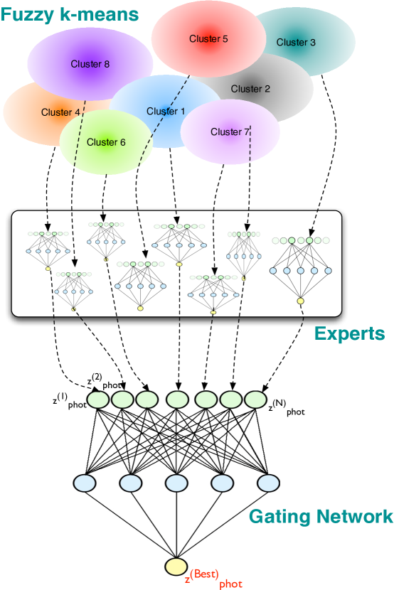
Figure 1: Diagram of the implementation of the WGE method described in this paper. The ellipses associated to the clusters in the features space have faded borders to stress the fuzzy nature of the clustering performed, while for the sake of simplicity, only one gating network of the committee of experts is shown.

4.1 Partitioning of the feature space

The gated experts method requires an unsupervised approach to the partitioning of the input space. It is well known that the color distribution of extragalactic sources changes noticeably with the redshift, so that it is possible to determine distinct regions of the features space where the color-redshift correlation follows different regimes.

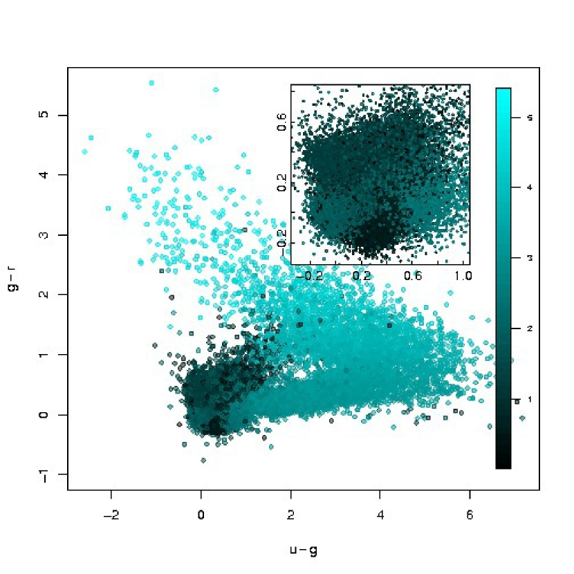
Figure 2: Spectroscopically selected quasars in the SDSS DR7 dataset in the $u-g$ vs $g-r$ plot. The color of the symbols is associated to the spectroscopic redshift of the sources.

For instance, in figure 2 it is shown the distribution of the sample of quasars observed spectroscopically by the SDSS in the DR7 in the $u\!-\!g$ vs $g\!-\!r$ color-color plot, where the color scale express the spectroscopic redshifts of the sources. Two main regions are clearly identified: a compact one where most of the objects lie, having redshifts in the interval $z_{\mathrm{spec}}\!=\![0,\sim\!2.5]$, and a vast region where the points are sparse and redshifts are larger than 2 with very few exceptions. From an astrophysical standpoint, this can be explained with the fact that the Lyman break at redshift $\sim 3$ enters the optical SDSS $u$ filter, in turn yielding larger values of the $u-g$ color.The inset zooms in the densest region of the plot, where most of the degeneracies arise. Although this plot shows a bi-dimensional projection of the 4-dimensional features space (where it is possible that some of the degeneracies are resolved), this particular window is characterized by sources with similar colors and very different redshifts. These facts suggest that it is possible to divide the input space into different regions, two or more inside the window and one or more outside. Even if it is unknown a priori whether the mapping function changes between these sub-domains, as it will be shown in paragraph 5.1, the error and noise regimes are different in such regions and, in particular, the densest ones are heavily affected by degeneracies while the others are mostly characterized by sparseness in the distribution of the points. In order to partition the input space, the implementation of the WGE method used for determination of the photometric redshifts employs a fuzzy version of a simple but effective clustering algorithm, namely the fuzzy $k$-means, or $c$-means [Dunn 1973]. The classical $k$-means algorithm (hereafter “sharp” k-means, opposed to the fuzzy counterpart), given the number of clusters $k$ and a metric definition, finds the centroids that minimize the distance with the objects belonging to their clusters while maximizing the distance among them by an iterative method. When convergence is reached, each point in the input space belongs to one and only one cluster. A different version of the sharp $k$-means algorithm, namely the $c$-means, works exactly like its sharp counterpart for what finding cluster centroids is concerned, except that, in this case, each source belonging to the input sample has a non-null probability of being a member of every cluster found by the algorithm, even of very distant ones. In particular, each point $x$ belongs to the $k$-th cluster (identified with its centroid $c_{k}$) with a membership degree $u_{k}(x)$ given by:

$$u_{k}(x)=\frac{1}{\sum_{j}\bigg{[}\frac{d(c_{k},x)}{d(c_{j},x)}\bigg{]}^{\frac{2}{(m-1)}}}$$ (13)

where $d(c_{k},x)$ is the distance of the point $x$ from the $k$-th cluster and $m$ is a positive integer, which determines the normalization of the coefficients of the clustering. In this paper, the parameter has been fixed to $m=2$ so that the “weights” associated to each cluster are a linear function of the distance from the center of the cluster and the sum of the coefficients is equal to 1. In practice, when partitioning the features space, all the points with membership degree larger than an arbitrary threshold have been assigned to each cluster. From a geometrical point of view, this allows to build clusters with soft boundaries, thus introducing some redundancy in the datasets and translates, in the case of the determination of photometric redshifts, into the fact that the same pattern is allowed to belong to different clusters, so that part of the information contained in each pattern is shared the different experts trained on each of these clusters. For a discussion on the choice of the optimal set of features, refer to paragraphs 5.1 and 6.

4.2 The gating network

Although the WGE architecture addresses by itself the bias variance trade-off problem, a MLP used as a gated network will introduce some variance and bias as well. This effect, mitigated by the WGE itself, is small but not negligible.In order to address this problem, we modeled the gating network as a committee of $N$ identical MLPs trained on the same dataset. Each network will produce a slightly different result/ The final prediction is the average of all the predictions. The choice of the number of MLPs has been made by considering the bias and the variance of two randomly chosen distribution of photometric redshifts for each experiment and for several different numbers of trainings of the gating network. The bias and variance for each couple of determinations of the photometric redshifts have been estimated using the mean and the standard deviation of the residual variable $\Delta z^{(phot)}$ between the two different determinations of the photometric redshifts:

$$\mathrm{bias}(z_{\mathrm{phot}}^{(1)},z_{\mathrm{phot}}^{(2)})=<\!\Delta_{z}^{(\mathrm{phot})}\!>=<\!(z_{\mathrm{photo}}^{(1)}-z_{\mathrm{photo}}^{(2)})\!>$$ (14)

$$\mathrm{var}(z_{\mathrm{phot}}^{(1)},z_{\mathrm{phot}}^{(2)})=\sigma_{\Delta_{z}^{(\mathrm{phot})}}=\sigma_{(z_{\mathrm{phot}}^{(1)}-z_{\mathrm{phot}}^{(2)})}$$ (15)

These two variables (normalized to unity) are plotted against the number of trainings of networks in the committee in plot 3. The optimal numbers of networks for the three experiments has been chosen as those numbers for which for the variations of the bias and variance were lower than 5% from the preceding realization, i.e. 30 gating network trainings for optical galaxies, 20 for optical quasars and 50 gating networks for optical and ultraviolet quasars. The same procedure was used to determine the optimal number of networks of the gating network for the determination of the errors on the photometric redshifts for each experiment. In this case, the threshold is reached is reached at 20 trainings for all experiments.

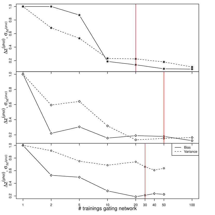
Figure 3: Normalized bias and variances for two randomly produced realizations of the photometric redshifts distributions as a function of the number of the trainings of the gating network. The values of the this number used for the experiments and the production of the catalogs is indicated by red horizontal lines. From top to bottom, optical quasars, optical+ultraviolet quasars and optical galaxies.

5 The knowledge bases and features selection

Three different KBs were employed during the training of the WGE method for the three classes of experiments performed, namely the evaluation of the photometric redshifts for:

• optical galaxies with spectroscopic redshifts;

• optical quasars with spectroscopic confirmation and redshift;

• optical+ultraviolet quasars spectroscopically confirmed.

The optical data for these three groups of experiments have all been extracted from the Sloan Digital Sky Survey (SDSS) DR7 database [Abazajian et al. 2009].The confirmed spectroscopic quasars with both optical and ultraviolet photometry, used for the third class of experiments, have been retrieved from the dataset of crossmatched sources from the SDSS and GALEX surveys [Budavari et al. 2009]. A more detailed description of the three KBs can be found below:

• 1^st KB (optical galaxies). It includes all primary extended SDSS sources classified as galaxies according to the SDSS specClass classification flag (specClass == $\{2\}$), having clean measured photometry in all filters $(u,g,r,i,z)$, reliable spectroscopic redshifts estimates and brighter than the completeness limit of the SDSS spectroscopic survey, namely 19.7 in the $r$ band. This sample, composed of $\sim 3.2\cdot 10^{5}$ sources, has been retrieved by querying the SDSS DR7 database for sources belonging to both $Galaxy$ and $SpecObjAll$ tables;

• 2^nd KB (optical quasars): all spectroscopically confirmed SDSS quasars (specClass == $\{3,4\}$), identified as point sources by any targeting program, with clean measured photometry in all filters $(u,g,r,i,z)$ and reliable spectroscopic redshifts estimates (this sample, composed of $\sim 7.5\!\cdot\!10^{4}$ sources, is a subset of the KB used for the extraction of candidate quasars described in 7.2.1). No specific cuts on the luminosity were performed. This sample has been retrieved by querying the SDSS DR7 database for sources belonging to the $SpecObjAll$ table;

• 3^rd KB (optical+ultraviolet quasars): all spectroscopically confirmed optical SDSS quasars ($\sim\!2.7\cdot\!10^{4}$ sources) associated to ultraviolet counterparts identified and observed by GALEX, with clean photometry in both optical $(u,g,r,i,z)$ and near and far ultraviolet bands $(nuv,fuv)$ and unambiguous positional cross-match (the sample of sources composing this KB is a proper subset of the second KB).

The queries used to extract the KBs from the SDSS and GALEX databases are reported in the appendix.

5.1 Features selection

The selection process of the photometric features used for the training of the WGE method (i.e. the features of the experiment) was based on the assumption that most of the information needed to reconstruct the photometric redshifts of extragalactic sources is encoded in the observed magnitudes [D’Abrusco et al. 2007]. However, since magnitudes are derived from fluxes, they tend to be correlated with each other and with the distance. Colors, instead, represent the ratio of fluxes measured in different filters and thus (once they have been corrected for extinction) they do not depend on the distance. Moreover, as it has already been discussed, the error regime changes with the redshift in the features space defined by the colors, thus encoding some information on the redshift which can be used to partially remove the degeneracy in the unknown colors-redshift relation. In figure 4, the distribution of the same sample of quasars spectroscopically selected in the SDSS DR7 used in figure 2, is plotted in the plane generated by the errors on the colors $u\!-\!g$ and $g\!-\!r$ evaluated by propagating the uncertainty on the individual magnitudes. Even if the correlation between the error distribution and spectroscopic redshifts is not as clear as in the case of the color-color plot shown before, also in this case low redshift sources are almost completely contained in a window corresponding to errors generally smaller than $0.2$ in both colors (the inset of the plots zooms into the high density region located in the left bottom corner). The other points are instead distributed in an elongated feature corresponding to low and almost constant error on the $\sigma_{g\!-\!r}$ parameter and varying $\sigma_{u\!-\!g}$. Finally, only a small number of sources is spread all over the plot and has significantly higher redshifts.

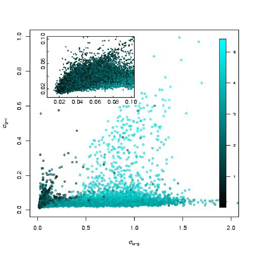
Figure 4: Spectroscopically selected quasars in the SDSS DR7 dataset in the $\sigma_{u-g}$ vs $\sigma_{g-r}$ plot. The color of the symbols is associated to the spectroscopic redshift of the sources.

In order to exploit all information contained in both the photometric features and their uncertainties, the experiments discussed in this paper used the errors on the photometric colors to perform the clustering, and both colors and their uncertainties for the training of the experts. More combinations of features and associated uncertainties were tested for each distinct experiment described here. All different combinations of features produced less accurate reconstructions of the photometric redshifts. In particular, using as parameters of the clustering the colors only or the colors and their errors yielded, on average, 10% larger MAD of the variable $\Delta z$ for all experiments.

For the first experiment involving the determination of the photometric redshifts for optical SDSS galaxies, the magnitudes used to derive the colors and their errors were the dereddened model magnitudes, i.e. the optimal estimates of the galaxy flux obtained by matching a spatial model to the source [Stoughton et al. 2002]. In this specific case, two different models are fitted to the two-dimensional images of each extended source in each band, namely a De Vaucouleurs profile and an exponential profile, and the best fitting model is used to calculate the model magnitude. The model magnitudes are then corrected for extinction according to the maps of galactic dust provided in [Schlegel et al. 1998]. For the samples of quasars used in the second an third experiments, the SDSS PSF magnitudes corrected for extinction were used to calculate optical colors and their uncertainties, while the remaining colors were calculated using the near and far ultraviolet magnitudes ($nuv$ and $fuv$ respectively) in the $PhotoObjAll$ table of the GALEX database [Budavari et al. 2009], containing the photometric attributes measured for the sources detected in the GALEX imagery.

6 The experiments

For each KB a distinct class of experiments was performed by varying some of the parameters of the WGE method, and the ones yielding the best results for each of those classes, in terms of the accuracy of the reconstruction of the photometric redshifts (according to the statistical diagnostics used to characterize the accuracy of the reconstruction and discussed in section 8), are described in the next three paragraphs. The outputs of three the best experiments were also used to produce the catalogs of photometric redshifts for SDSS galaxies and candidate quasars, described respectively in sections 7.1, 7.2 and 7.3. In this section, the accuracy of the reconstruction of the photometric redshifts will be expressed by the robust estimates of the scattering of the variable $\Delta z\!=\!z_{\mathrm{phot}}\!-\!z_{\mathrm{spec}}$, evaluated through its median absolute deviation (hereafter MAD). Given a univariate set of variables $\{\Delta z^{(1)},\Delta z^{(2)},...,\Delta z^{(N)}\}$, the MAD of this sample is defined as:

$$\mathrm{MAD(\Delta z)}=\mathrm{median}(\Delta z-\mathrm{median}(\Delta z))$$ (16)

In other words, MAD is the median of the absolute deviation of the residuals from the median of the residuals itself. A modified version of the standard MAD statistics (hereafter MAD^′) that can be used for the evaluation of the accuracy of the reconstruction of the photometric redshifts can be defined for the $\Delta z$ variable as follows:

$$\mathbf{\mathrm{MAD^{\prime}(\mathrm{\Delta z})}=\mathrm{median}(\|\Delta z\|)}$$ (17)

A summary of the features used for the estimation of photometric redshifts and the errors on the photometric redshifts in these experiments are shown in tables LABEL:table:experiments and LABEL:table:experimentserr respectively, while the physical motivation behind the selection of the features used to train the WGE method has been given in the subsection 5.1. A more detailed characterization of the accuracy of the photometric redshifts reconstruction, obtained by means of distinct global and redshift-dependent statistical diagnostics, is discussed in paragraph 8.

The criteria used for the choice of the best experiments for each class of experiments are the following, in order of decreasing priority:

• The total percentages of test-set sources with $\|\Delta z\|<0.01$, $\|\Delta z\|<0.02$ and $\|\Delta z\|<0.03$ respectively ($<\!0.3$, $<\!0.2$ and $<\!0.1$ for the experiments involving quasars). These quantities, hereafter, will be referred to as $\Delta z_{1}$, $\Delta z_{2}$ and $\Delta z_{3}$ for galaxies and quasars as well;

• The value of the $MAD$ diagnostic of the $\Delta z$ variable as defined in equation 16;

• The value of the $MAD^{\prime}$ diagnostic of the $\Delta z$ variable as defined in equation 17;

While the main criterion to select the best experiment is the first and the other two were used as tie-breakers in case of equal value of $\Delta z_{1}$, $\Delta z_{2}$ and $\Delta z_{3}$ (with a tolerance of 0.1%), for all classes of experiments the best one has been unambiguously selected by each of these criteria separately, as shown in figure 5. In this plot, the values of the three diagnostics are shown respectively for all experiments of each class considered in this paper (optical galaxies, optical quasars and optical+ultraviolet quasars), as a function of the number of clusterings.

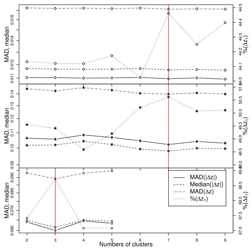
Figure 5: Statistical diagnostics as a function of the number of fuzzy clusters for the three experiments described in this paper (from the upper to lower panel, the experiments for the determination of the photometric redshifts of optical galaxies, quasars with optical photometry and quasars with optical and ultraviolet photometry). The optimal number of clusters, as reported in table LABEL:table:experiments, are marked with a red vertical line. In all cases, the optimal number of clusters are associated to the highest values of the $\%(\Delta z_{1})$ variable and to the lowest values of the three diagnostics MAD, MAD’ and ${\mathrm{m}edian}(\|\Delta z\|)$.

Table 1: Parameters of the best experiments for the evaluation of the photometric redshifts for optical galaxies, optical candidate quasars and optical plus ultraviolet candidate quasars.

Parameters	Optical Galaxies	Optical Quasars	Optical+UV Quasars
Params. clustering	$\sigma_{u\!-\!g}$, $\sigma_{g\!-\!r}$, $\sigma_{r\!-\!i}$, $\sigma_{i\!-\!z}$	$\sigma_{u\!-\!g}$, $\sigma_{g\!-\!r}$, $\sigma_{r\!-\!i}$, $\sigma_{i\!-\!z}$	$\sigma_{u\!-\!g}$,$\sigma_{g\!-\!r}$,$\sigma_{r\!-\!i}$,$\sigma_{i\!-\!z}$,
			$\sigma_{fuv\!-\!nuv}$,$\sigma_{nuv\!-\!u}$
Min. # clusters	5	2	2
Max. # clusters	9	9	9
Opt. # clusters	7	7	3
Clusters threshold	0.15	0.1	0.1
Max. iterations clust.	500	500	500
Params. experts	$\sigma_{u\!-\!g}$,$\sigma_{g\!-\!r}$,$\sigma_{r\!-\!i}$,$\sigma_{i\!-\!z}$,	$\sigma_{u\!-\!g}$,$\sigma_{g\!-\!r}$,$\sigma_{r\!-\!i}$,$\sigma_{i\!-\!z}$,	$\sigma_{u\!-\!g}$,$\sigma_{g\!-\!r}$,$\sigma_{r\!-\!i}$,$\sigma_{i\!-\!z}$,
	$(u\!-\!g)$,$(g\!-\!r)$,$(r\!-\!i)$,$(i\!-\!z)$	$(u\!-\!g)$,$(g\!-\!r)$,$(r\!-\!i)$,$(i\!-\!z)$	$\sigma_{fuv\!-\!nuv}$,$\sigma_{nuv\!-\!u}$,
			$(fuv\!-\!nuv)$,$(nuv\!-\!u)$,$(u\!-\!g)$,
			$(g\!-\!r)$,$(r\!-\!i)$,$(i\!-\!z)$
Hid. neurons experts	30	20	20
Max. epochs. experts	500	500	500
Learning rate experts	0.01	0.01	0.01
Steepness experts	1.0	1.0	1.0
Hid. neurons gate	30	20	20
Max. epochs. gate	500	500	500
Learning rate gate	0.01	0.01	0.01
Steepness gate	1.0	1.0	1.0
# training gates	30	20	50

A first set of experiments were performed in order to set the steepness and the learning rate for all the experts in the whole features space. Once set, these values have not been treated as parameters of the WGE training but are considered fixed. Moreover, different values of the two parameters for the gating network have been explored, leading to a negligible variation in the final estimates of the photometric redshifts and associated errors. For this reason, the values determined for the experts were used for all experiments.

6.1 Photometric redshifts of galaxies with optical photometry

The best experiment for the evaluation of the photometric redshifts of optical galaxies, retrieved from the SDSS photometric database, has been performed using the four SDSS colors and the corresponding errors (obtained by propagating the errors on the single magnitudes) as features and the spectroscopic redshifts measured by the SDSS spectroscopic pipelines as target. The training of the WGE method, as described in detail in section 3, is obtained by first performing a clustering in the features space and then training the single experts on each of the clusters, so that the final outcome of the method is evaluated by the gating network which combines the distinct outputs from the experts. For this experiment, the c-means clustering has been performed on the distribution of KB sources in the 4-dimensional features space based on the uncertainties of the photometric colors $\sigma_{u\!-\!g}$, $\sigma_{g\!-\!r}$, $\sigma_{r\!-\!i}$ and $\sigma_{i\!-\!z}$, calculated by propagating the statistical uncertainties on the single magnitudes. The single experts have been trained on the different clusters determined by the fuzzy K-means algorithm in the 8-dimensional photometric features space obtained by adding the four colors $u\!-\!g$, $g\!-\!r$, $g\!-\!r$ and $i\!-\!z$ to their uncertainties $\sigma_{u\!-\!g}$, $\sigma_{g\!-\!r}$, $\sigma_{r\!-\!i}$ and $\sigma_{i\!-\!z}$.

After multiple experiments performed with different values of the parameters of the WGE method, the optimal value of the membership threshold on the fuzzy clustering has been fixed to $0.1$, so that each source has been considered member only of the clusters which accounts for at least $10\%$ of its total membership. The global MAD of the $\Delta z$ variable of this experiment is 0.017. The scatterplot showing the distribution of photometric redshifts against the corresponding spectroscopic redshifts for the members of the KB used for test the WGE method for the catalog of galaxies extracted from the SDSS DR7 database is shown in figure 6. The histograms of the distributions of both photometric and spectroscopic redshifts for the test set of this experiment are shown in figure 9.

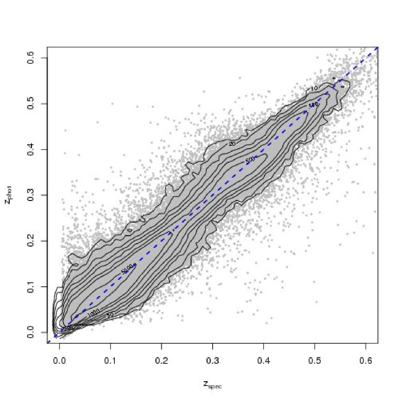
Figure 6: Scatterplot of the spectroscopic redshifts vs photometric redshifts with isodensity contours for the sample of SDSS galaxies with optical photometry, belonging to the KB used to train the WGE in the first experiment. The isodensity contours are drawn for the following sequence of density values: $\{10,20,50,100,200,500,1000,5000\}$.

Figure 7: Histograms of the distribution of spectroscopic and photometric redshifts for the sample of SDSS galaxies with optical photometry, belonging to the KB used to train the WGE in the first experiment.

6.2 Photometric redshifts of quasars with optical photometry

The best experiment for the evaluation of the photometric redshifts of optical confirmed quasars extracted from the SDSS spectroscopic database made use of the four SDSS colors and associated uncertainties as features, and of the SDSS spectroscopic redshifts as targets. Similarly to what was described for the first experiment, the first step of the WGE training involved the determination of the optimal clustering of the KB sources in the 4-dimensional feature space consisting of the errors of the colors $\sigma_{u\!-\!g}$, $\sigma_{g\!-\!r}$, $\sigma_{r\!-\!i}$ and $\sigma_{i\!-\!z}$. On the other hand, the experts and the gating expert have been trained on the whole 8-dimensional feature space generated by the 4 optical colors and their uncertainties. After multiple runs of the WGE method with different values of the parameters, the optimal value of the threshold on the fuzzy clustering has been fixed to 0.15. The clustering of the experiment for the determination of the errors on the photometric redshifts was carried out using, as features, the whole set of 8 photometric features mentioned above in addition to the photometric redshifts $z_{\mathrm{phot}}$ and the variable $\Delta z$. The global MAD of the $\Delta z$ variable of this experiment is 0.14. The scatterplot of the distribution of photometric redshifts against the spectroscopic redshifts for the KB used to train the WGE method in this experiment is shown in figure 8, while the histograms of both spectroscopic and photometric redshifts distribution are shown in figure 9.

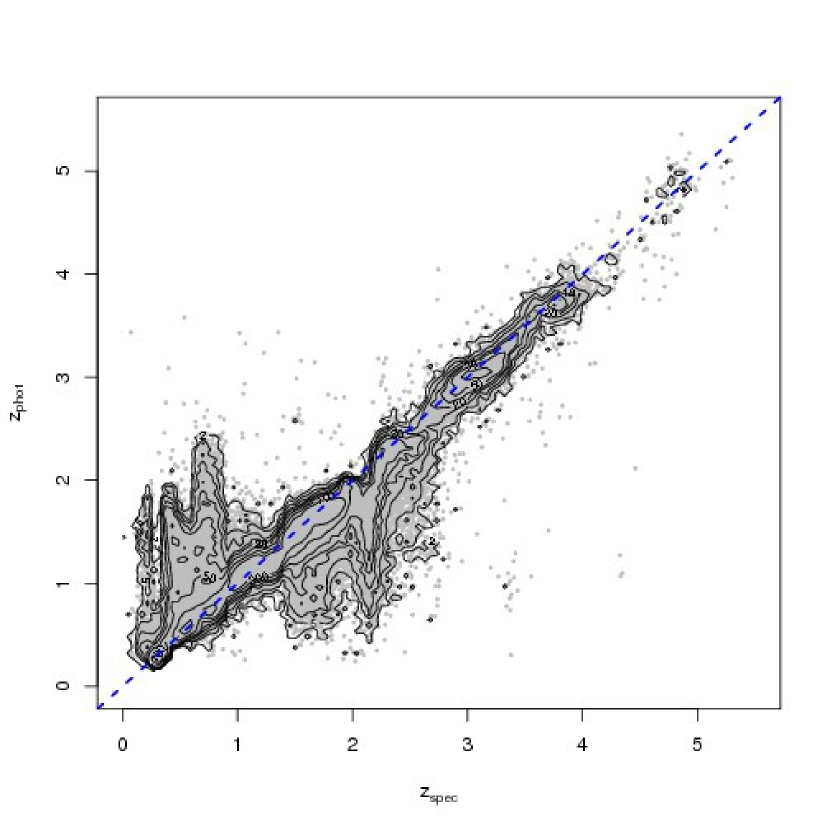
Figure 8: Scatterplot of the spectroscopic redshifts vs photometric redshifts with isodensity contours for the sample of SDSS quasars with optical photometry, belonging to the KB used to train the WGE in the second experiment. The isodensity contours are drawn for the following sequence of density values: $\{2,5,10,20,30,50,100,200\}$.

Figure 9: Histograms of the distribution of spectroscopic and photometric redshifts for the sample of SDSS quasars with optical photometry, belonging to the KB used to train the WGE in the second experiment.

6.3 Photometric redshifts of quasars with optical and ultraviolet photometry

The most accurate reconstruction of the photometric redshifts for the quasars with SDSS optical and GALEX ultraviolet photometric data was achieved using, as features for the clustering, the 6 uncertainties of the colors obtained by combining the 5 SDSS optical filters and the 2 ultraviolet filters and by propagating the statistical errors on the magnitudes.

The training of the experts and the gating expert was therefore carried out on the whole set of photometric features available, i.e. the errors $\sigma_{u\!-\!g}$, $\sigma_{g\!-\!r}$, $\sigma_{r\!-\!i}$, $\sigma_{i\!-\!z}$, $\sigma_{fuv\!-\!nuv}$, $\sigma_{nuv\!-\!u}$ and the colors $(u\!-\!g)$,$(g\!-\!r)$,$(r\!-\!i)$,$(i\!-\!z)$,$(fuv\!-\!nuv)$,$(nuv\!-\!u)$. Also in this experiment, the clustering for the determination of the errors on the photometric redshifts was performed inside the feature space generated by the whole set of photometric features used for the estimation of the photometric redshifts in addition to the photometric redshift $z_{\mathrm{phot}}$ itself and to the variable $\Delta z$. The MAD of the final $\Delta z$ variable in this experiment is 0.09, improving noticeably the accuracy of the photometric redshifts reconstruction obtained with the optical photometry only. As in the previous two experiments, the scatterplot of the distribution of photometric redshifts against the spectroscopic redshifts for the sources of the KB used to test the WGE method in this experiment is shown in figure 10, while the histograms of both photometric and spectroscopic redshifts are shown in figure 11.

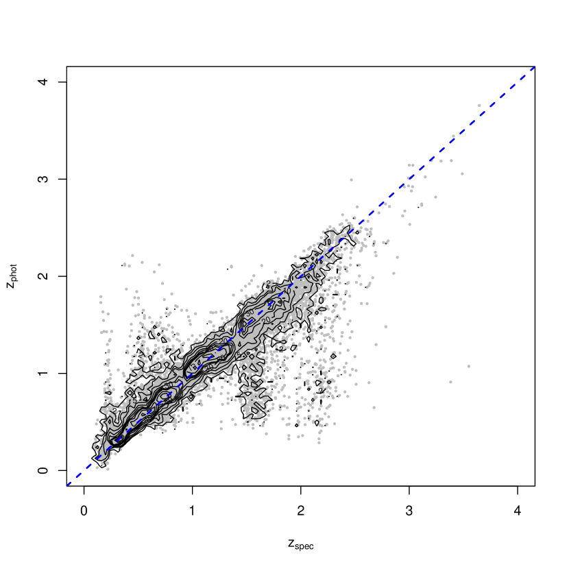
Figure 10: Scatterplot of the spectroscopic redshifts vs photometric redshifts with isodensity contours for sample of quasars with optical and ultraviolet photometry, belonging to the KB used to train the WGE in the third experiment. The isodensity contours are drawn for the following sequence of density values: $\{2,5,10,20,30,40,50,75,100,150,200\}$.

Figure 11: Histograms of the distribution of spectroscopic and photometric redshifts for the sample of SDSS quasars with optical and ultraviolet photometry, belonging to the KB used to train the WGE in the third experiment.

7 The catalogs

7.1 The catalog of photometric redshifts for SDSS galaxies

A catalog of photometric redshifts for a sample of galaxies extracted from the SDSS-DR7 database has been produced using the model obtained by training the WGE as described in section 6.1. The photometric galaxies were extracted, in a similar way to what done for the KB used for the training experiment, by querying the Galaxy table of the SDSS database for all primary extended sources with clean photometry in all filters $(u,g,r,i,z)$, and brighter than 21.0 in the $r$ band (the SQL query is shown in the appendix A).

In total, the catalog contains photometric redshifts for $\sim 3.2\cdot 10^{7}$ sources. The set of specific features used for the evaluation of photometric redshifts, the estimated photometric redshifts values, errors and diagnostics flag together with some of the most common observational parameters retrieved directly from the SDSS database and useful for the identification of the sources in the SDSS database, have been included in the catalog for the sake of completeness. More information about the 24 columns of the catalog format are given in table LABEL:table:catgal. The photometric redshifts and uncertainties from our catalogs will also be incorporated into the NASA/IPAC Extragalactic Database (NED) services.

Table 2: Columns of the catalog of galaxies extracted from the SDSS with photometric redshifts evaluated using optical photometry.

#	Name	Type	Description
1	objID	Long	unique SDSS object ID
2	ra	Double	right ascension in degrees (J2000)
3	dec	Double	declination in degrees (J2000)
4	dered_u	Float	SDSS dereddened $u$ model mag
5	dered_g	Float	SDSS dereddened $g$ model mag
6	dered_r	Float	SDSS dereddened $r$ model mag
7	dered_i	Float	SDSS dereddened $i$ model mag
8	dered_z	Float	SDSS dereddened $z$ model mag
9	modelmagerr_u	Float	SDSS $u$ model mag error
10	modelmagerr_g	Float	SDSS $g$ model mag error
11	modelmagerr_r	Float	SDSS $r$ model mag error
12	modelmagerr_i	Float	SDSS $i$ model mag error
13	modelmagerr_z	Float	SDSS $z$ model mag error
14	extinction_u	Float	SDSS $u$ mag extinction
15	extinction_g	Float	SDSS $g$ mag extinction
16	extinction_r	Float	SDSS $r$ mag extinction
17	extinction_i	Float	SDSS $i$ mag extinction
18	extinction_z	Float	SDSS $z$ mag extinction
19	u-g	Double	$u-g$ color
20	g-r	Double	$g-r$ color
21	r-i	Double	$r-i$ color
22	i-z	Double	$i-z$ color
23	photoz	Double	photometric redshift
24	photoz_err	Double	photometric redshift error

7.1.1 Contamination of the catalog of photometric redshifts for SDSS galaxies

The redshift distribution of the sources belonging to the KB used to train the WGE for the determination of the catalog of photometric redshifts for the galaxies extracted from the SDSS DR7, is shown in figure 7. Even though no constraints on the redshift of the sources were explicitly required (as it is clear from the SQL version of the query in appendix A), all galaxies belonging to this KB have spectroscopic redshift $z\!<0.6$. A certain degree of contamination from galaxies at redshift $z\!>0.6$ (and for this reason, not represented in the KB used for the WGE training) is expected in the catalog of photometric redshifts evaluated for the photometric galaxies extracted from the SDSS database. These galaxies could be mistakenly assigned a wrong value of their photometric redshift, in some case significantly lower than their real redshift. The number and distribution of such galaxies, hereafter called contaminants, can be statistically evaluated either by using the luminosity function of the same galaxy population in the same band, similarly to what has been done in [D’Abrusco et al. 2007], or by employing a deeper catalog of galaxies with reliable measures of the redshifts. In the case of the catalog discussed in this section, the second method has been chosen to evaluate the contamination from high redshifts galaxies, using data from the DEEP2 survey [Davis et al. 2007]. DEEP2 is a spectroscopic survey that provides the most detailed census of the galaxy distribution at $z_{\mathrm{spec}}\!\sim\!1$, targeting $\sim\!5.0\!\cdot 10^{5}$ galaxies in the redshift range $0\!<\!z\!<\!1.4$. The last data release (DR3) includes redshifts spanning four survey fields overlapping with the SDSS sky coverage. The SDSS galaxies with photometric redshifts estimated with the WGE method have been positionally crossmatched with the catalog DEEP2 DR3 catalog of sources. The sample of cross-identified galaxies has been used to produce figure 12, which shows the distribution of contaminants as functions of the apparent magnitude in the $r$ SDSS filter after correction for the extinction and the the photometric redshift $z_{\mathrm{phot}}$ of the galaxies. The fraction of contaminants is zero for $r$ magnitude smaller than 19 and is smaller than 20$\%$ for $r\!<\!20.5$. On the other hand, the fraction of contaminants as a function of the values of the photometric redshifts assigned by the WGE method is consistently lower than 15$\%$ for $z_{\mathrm{phot}}\!<\!0.55$. Uncertainties on the quantities plotted in the figure 12 have been evaluated applying poissonian statistics, and the large error bars for low magnitudes are caused by low statistics.

Figure 12: Fraction of contaminants (galaxies with $z_{\mathrm{spec}}>0.6$) in the catalog of SDSS DR7 photometric galaxies with photometric redshifts evaluated with the WGE method as function of the apparent magnitude in the $r$ band (black symbols) and photometric redshifts (red symbols).

7.2 The catalog of photometric redshifts for SDSS optical candidate quasars

A catalog of photometric redshifts for the optical candidate quasars extracted from the SDSS-DR7 database is described in [D’Abrusco et al. 2009]. The photometric redshifts for this sample of candidate quasars have been evaluated using the results of the WGE training experiment described in the section 6.2. The sample of point-like sources in the table PhotoObjAll of the SDSS-DR7 database from which the candidate quasars were extracted is composed of all the primary photometric stellar sources (using the SDSS ’type’ flag, which provides a morphological classification of the sources by classifying them as extended or point-like) with clean photometry in all the filters $(u,g,r,i,z)$ and brighter than 21.3 in the $i$ band, for consistency with the sample of sources selected in [Richards et al. 2009]. The SQL query used to retrieve the data is given in the appendix B. The catalog retains the same basic structure of the catalog of photometric redshifts of galaxies, with few changes. This catalog contains $\sim 2.1\cdot 10^{6}$ candidate quasars, and consists of the list of candidate quasars with a small set of photometric features used for the extraction process, with additional quantities derived by the method for the extraction of the candidates and the evaluation of photometric redshifts. Also in this case, some of the most common observational parameters available in the SDSS database were retrieved and added to the catalog to allow easier cross-matching with the original SDSS database. More detailed information about the 31 columns of the catalog of photometric redshifts for the optical candidate quasars extracted from the SDSS-DR7 database are presented in table LABEL:table:catqsos. For this catalog a cone search service compliant with the VO standards will be made available as well.

Table 3: Columns of the catalog of candidate quasars with photometric redshifts evaluated using optical photometry

#	Name	Type	Description
1	catjID	Long	unique catalog object ID
2	objID	Long	unique SDSS object ID
3	ra	Double	right ascension in degrees (J2000)
4	dec	Double	declination in degrees (J2000)
5	psfMag_u	Float	SDSS PSF $u$ model mag
6	psfMag_g	Float	SDSS PSF $g$ model mag
7	psfMag_r	Float	SDSS PSF $r$ model mag
8	psfMag_i	Float	SDSS PSF $i$ model mag
9	psfMag_z	Float	SDSS PSF $z$ model mag
10	psfmagerr_u	Float	SDSS $u$ PSF mag error
11	psfmagerr_g	Float	SDSS $g$ PSF mag error
12	psfmagerr_r	Float	SDSS $r$ PSF mag error
13	psfmagerr_i	Float	SDSS $i$ PSF mag error
14	psfmagerr_z	Float	SDSS $z$ PSF mag error
15	extinction_u	Float	SDSS $u$ mag extinction
16	extinction_g	Float	SDSS $g$ mag extinction
17	extinction_r	Float	SDSS $r$ mag extinction
18	extinction_i	Float	SDSS $i$ mag extinction
19	extinction_z	Float	SDSS $z$ mag extinction
20	strID	Long	SDSS stripe ID
21	u-g	Double	$u-g$ color
22	g-r	Double	$g-r$ color
23	r-i	Double	$r-i$ color
24	i-z	Double	$i-z$ color
25	cluID	Integer	cluster ID
26	densKDEqsos	Double	KDE estimated p.d.f. relative to quasars distr.
27	densKDEnotqsos	Double	KDE estimated p.d.f. relative to not-quasars distr.
28	densKDEratio	Double	KDE estimated p.d.f. for quasars distr. to KDE
			estimated p.d.f. for not quasars distr. ratio
29	photoz	Double	photometric redshift (opt.+UV)
30	photoz_err	Double	photometric redshift error
31	photoz_flag	Short	photometric redshift flag

7.2.1 Candidate quasars

The WGE method has been used to estimate photometric redshifts for the members of an updated version of the SDSS catalog of optical candidate quasars described in [D’Abrusco et al. 2009]. While referring to the original work for a detailed description of the statistical method employed for the extraction of the candidate quasars, here we shall shortly summarize its basic facts in order to introduce some additional parameters included in the catalog. The method used to produce the catalog of candidate quasars relies on the geometrical characterization of the distribution of spectroscopically confirmed quasars in the optical photometric features space and employs a combination of clustering techniques to achieve the best possible separation between regions of the features space dominated by stars and quasars respectively. The method is based on the combination of different DM algorithms since it includes a dimensionality reduction phase obtained via Probabilistic Principle Surfaces (PPS) followed by a clustering performed using the Negative Entropy Clustering (NEC) respectively. The method allows to determine the salient correlations between the distribution of confirmed quasars in the photometric features space and to use this information to extract new photometric candidate quasars. Given the original KB (a sample of point-like sources with spectroscopic classification), the extraction of the candidate quasars is performed by associating each photometric source to the closest cluster and retaining as candidates only those sources associated to clusters dominated by confirmed quasars. In the revised version of the catalog, the information provided for each candidate quasar has been completed by three parameters, namely the probabilities of each candidate quasar of being extracted from the underlying distributions of confirmed quasars or stars, and the ratio of these two probabilities. The first two values have been extracted from the probability density functions (pdf) associated to the two distinct distributions of stars and quasars, obtained by applying the Kernel Density Estimation (KDE) method. These parameters can be used to further refine the efficiency of the selection, at the cost of reducing the completeness of the sample. The catalog has been extracted from the DR7 SDSS database, thus yielding $\sim\!15\%$ more sources than the first version of the catalog.

7.3 The catalog of photometric redshifts for SDSS optical and ultraviolet candidate quasars

A third catalog containing photometric redshifts estimates for a subsample of optical candidate quasars described in 7.2.1 for which ultraviolet photometry from GALEX is available has been produced by using the results of the WGE training experiment described in the section 6.3. The photometric redshifts for quasars with both optical and ultraviolet photometry are significantly more accurate that those evaluated using optical photometry only, and the fraction of catastrophic outliers is reduced as well (as will be described in detail in section 8). This catalog contains $\sim 1.6\cdot 10^{5}$ sources. The query used to retrieve the ultraviolet photometry of the sources with reliable GALEX counterparts is shown in appendix C. The columns contained in the catalog are described in table LABEL:table:catqsosuv. Also in this case, the catalog will be available through a cone search service.

Table 4: Columns of the catalog of candidate quasars with photometric redshifts evaluated using optical and ultraviolet photometry.

#	Name	Type	Description
1	catjID	Long	unique catalog object ID
2	objIDsdss	Long	unique SDSS object ID
3	objIDgal	Long	unique GALEX object ID
4	ra	Double	right ascension in degrees (J2000)
5	dec	Double	declination in degrees (J2000)
6	nuv	Float	GALEX $nuv$ mag
7	fuv	Float	GALEX $fuv$ mag
8	psfMag_u	Float	SDSS PSF $u$ model mag
9	psfMag_g	Float	SDSS PSF $g$ model mag
10	psfMag_r	Float	SDSS PSF $r$ model mag
11	psfMag_i	Float	SDSS PSF $i$ model mag
12	psfMag_z	Float	SDSS PSF $z$ model mag
13	magerr_nuv	Float	GALEX $nuv$ mag error
14	magerr_fuv	Float	GALEX $fuv$ mag error
15	psfmagerr_u	Float	SDSS $u$ PSF mag error
16	psfmagerr_g	Float	SDSS $g$ PSF mag error
17	psfmagerr_r	Float	SDSS $r$ PSF mag error
18	psfmagerr_i	Float	SDSS $i$ PSF mag error
19	psfmagerr_z	Float	SDSS $z$ PSF mag error
20	extinction_u	Float	SDSS $u$ mag extinction
21	extinction_g	Float	SDSS $g$ mag extinction
22	extinction_r	Float	SDSS $r$ mag extinction
23	extinction_i	Float	SDSS $i$ mag extinction
24	extinction_z	Float	SDSS $z$ mag extinction
25	strID	Long	SDSS stripe ID
26	fuv-nuv	Double	$fuv-nuv$ color
27	nuv-u	Double	$nuv-u$ color
28	u-g	Double	$u-g$ color
29	u-g	Double	$u-g$ color
30	g-r	Double	$g-r$ color
31	r-i	Double	$r-i$ color
32	i-z	Double	$i-z$ color
33	cluID	Integer	cluster ID
34	densKDEqsos	Double	KDE estimated p.d.f. relative to quasars distr.
35	densKDEnotqsos	Double	KDE estimated p.d.f. relative to not-quasars distr.
36	densKDEratio	Double	KDE estimated p.d.f. for quasars distr. to KDE
			estimated p.d.f. for not quasars distr. ratio
37	photoz	Double	photometric redshift (opt.+UV)
38	photoz_err	Double	photometric redshift error
39	photoz_flag	Short	photometric redshift flag

8 Accuracy of the photometric redshift reconstruction

Many different statistical diagnostics have been used in the literature to characterize the reconstruction of photometric redshifts as a function of the observational features used to evaluate the quality of the redshifts. In this paragraph, a thorough statistical description of the performance of the WGE method will be given, in terms of the accuracy of the reconstruction, the biases of the reconstructed distribution of photometric redshifts and the fraction of outliers. A comparison of our results with others drawn from the literature is also provided in table LABEL:table:diagnostics, along with a comprehensive set of statistical diagnostics evaluated for the three different classes of experiments performed with the WGE method. All statistics have been calculated for the variables $\Delta z$ and $\Delta z_{\mathrm{norm}}=\frac{\Delta z}{1+z_{\mathrm{spec}}}=\frac{z_{\mathrm{phot}}-z_{\mathrm{spec}}}{1+z_{\mathrm{spec}}}$.

The statistical diagnostics evaluated for the results of the three experiments are the following:

• the averages $<\Delta z>$ and $<\Delta z_{\mathrm{norm}}>$ of both $\Delta z$ and $\Delta z_{\mathrm{norm}}$ variables, which accounts for the overall bias of the photometric redshifts distribution;

• the Root Mean Square (RMS) of both variables $\Delta z$ and $\Delta z_{\mathrm{norm}}$, defined respectively as:

  $$RMS(\Delta z)=\sqrt{\sum(\Delta z)^{2}/N}$$ (18)

  $$RMS(\Delta z_{\mathrm{norm}})=\sqrt{\sum(\Delta z_{\mathrm{norm}})^{2}/N}$$ (19)

  where N is the total number of values. The RMS accounts for the overall variation of the photometric redshifts distribution compared to the spectroscopic redshifts distribution;

• the variances $\sigma^{2}(\Delta z)$ and $\sigma^{2}(\Delta z_{\mathrm{norm}})$ and the MAD of both $\Delta z$ and $\Delta z_{\mathrm{norm}}$ variables, accounting for the accuracy of the reconstruction measured as the spread of the two different variables;

• the values of the $MAD^{\prime}$ for both $\Delta z$ and $\Delta z_{\mathrm{norm}}$ variables;

• the percentage of sources with $\Delta z\!<\!\{\Delta z_{1}=0.01,\Delta z_{2}=0.02,\Delta z_{3}=0.03\}$ and $\Delta z\!<\!\{\Delta z_{1}=0.1,\Delta z_{2}=0.2,\Delta z_{3}=0.3\}$ for the experiments involving galaxy and quasars respectively (hereafter $\Delta z_{1}$, $\Delta z_{2}$ and $\Delta z_{3}$ will be used for both galaxies and quasars, while $\Delta z_{\mathrm{norm},1}$, $\Delta z_{\mathrm{norm},2}$ and $\Delta z_{\mathrm{norm},3}$ will be used with the same meaning for the $\Delta z_{\mathrm{norm}}$ variable), which provide estimates of the performances of the reconstruction process at different levels of accuracy;

• the variance for the sources at $\Delta z_{1}$, $\Delta z_{2}$ and $\Delta z_{3}$ ($\Delta z_{\mathrm{norm},1}$, $\Delta z_{\mathrm{norm},2}$ and $\Delta z_{\mathrm{norm},3}$), that represents an alternative measure of the performance of the reconstruction at three different levels of the accuracy;

In table LABEL:table:diagnostics we show the values of such diagnostics for the three experiments described in this paper and for a few other relevant papers in the literature that apply different methods to similar KBs and photometric datasets (wide band photometry from ground based surveys in the optical and ultraviolet surveys). Namely, the results from [Ball et al. 2008, Richards et al. 2009] for quasars with either optical or optical+ultraviolet photometry, and [D’Abrusco et al. 2007] for optical galaxies are reported in the table. The WGE method noticeably improves over the accuracy achieved by [D’Abrusco et al. 2007] in the reconstruction of the photometric redshifts for SDSS galaxies according to all the diagnostics, with only slightly smaller fractions of sources within $\Delta z_{1}$, $\Delta z_{2}$ and $\Delta z_{3}$. In the case of the determination of the photometric redshifts for optical quasars, the kNN method used in [Ball et al. 2008] (column (2)) achieves a much larger variance for the $\Delta z$ variable while performing very similarly at the WGE method in terms of $\Delta z_{1}$, $\Delta z_{2}$ and $\Delta z_{3}$, bias and variance of the distribution of $\Delta z_{\mathrm{norm}}$ variable. Similar results are achieved by the two methods also for the reconstruction of the photometric redshifts of quasars extracted from the SDSS with both optical and ultraviolet photometry, except for the fact that kNN achieves a much better variance for the distribution of the variable $\Delta z_{\mathrm{norm}}$. A different approach, not based on machine learning techniques, but similarly aimed at the determination of the empirical correlation between the colors and redshifts of the sources for the evaluation of the photometric redshifts is adopted in [Richards et al. 2009] (CZR method). Some of the diagnostics available for the application of this method to SDSS quasars with both optical and optical+ultraviolet photometry show that such mok ethod achieves consistently lower accuracy relative to both WGE and kNN methods (with the exception of the normalized variance for optical+UV experiment), while providing slightly larger fraction of sources within $\Delta z_{1}$, $\Delta z_{2}$ and $\Delta z_{3}$ in the case of optical quasars.

Table 5: Statistical diagnostics of photometric redshifts reconstruction for all the experiments discussed in this paper and for relevant papers in the literature. The first column (Exp. 1) contains the diagnostics for the experiment for the determination of the photometric redshifts of the optical galaxies from the SDSS catalog described in paragraph 6.1, while the columns (Exp. 2) and (Exp. 3) describe the diagnostics for the experiments concerning the determination of the photometric redshifts for quasars with optical and optical+ultraviolet photometry respectively (the details can be found in paragraphs 6.2 and 6.3). The same statistical diagnostics are shown for some papers from the literature, respectively [D’Abrusco et al. 2007] for optical galaxies in column (1) and both [Ball et al. 2008] and [Richards et al. 2009] for optical and optical+ultraviolet quasars in the columns (2) and (3) respectively (as reported in [Ball et al. 2008]). The definitions of the statistical diagnostics and other relevant

results of the literature are discussed in section 8. Diagnostic Exp. 1 (1) Exp. 2 (2) (3) Exp. 3 (2) (3) $\left\langle\Delta z\right\rangle$ 0.015 0.021 0.21 - - 0.13 - - RMS$(\Delta z)$ 0.021 0.074 0.35 - - 0.25 - - $\sigma^{2}(\Delta z)$ $2.3\!\cdot\!10^{-4}$ $5.0\!\cdot\!10^{-4}$ 0.08 0.123 0.27 0.044 0.054 0.136 MAD$(\Delta z)$ 0.011 0.012 0.11 - - 0.061 - - MAD’$(\Delta z)$ $\mathbf{0.012}$ - $\mathbf{0.098}$ - - $\mathbf{0.062}$ - - $\%(\Delta z_{1})$ 43.4 41.1 50.7 54.9 63.9 68.1 70.8 74.9 $\%(\Delta z_{2})$ 72.4 68.4 72.3 73.3 80.2 86.5 85.8 86.9 $\%(\Delta z_{3})$ 86.9 83.4 80.5 80.7 85.7 91.4 90.8 91.0 $\sigma^{2}(\Delta z_{1})$ $8.2\!\cdot\!10^{-6}$ $8.2\!\cdot\!10^{-6}$ $7.9\!\cdot\!10^{-4}$ - - $7.6\!\cdot\!10^{-4}$ - - $\sigma^{2}(\Delta z_{2})$ $3.0\!\cdot\!10^{-5}$ $3.1\!\cdot\!10^{-5}$ 0.003 - - 0.023 - - $\sigma^{2}(\Delta z_{3})$ $6.1\!\cdot\!10^{-5}$ $6.3\!\cdot\!10^{-5}$ 0.005 - - 0.039 - - $\left\langle\Delta z_{\mathrm{norm}}\right\rangle$ 0.014 0.017 0.095 0.095 0.115 0.058 0.06 0.071 RMS$(\Delta_{\mathrm{norm}})$ 0.019 0.037 0.19 - - 0.11 - - $\sigma^{2}(\Delta z_{\mathrm{norm}})$ $1.8\!\cdot\!10^{-4}$ $1.1\!\cdot\!10^{-3}$ 0.025 0.034 0.079 0.086 0.014 0.031 MAD$(\Delta z_{\mathrm{norm}})$ 0.009 0.011 0.041 - - 0.029 - - MAD’$(\Delta z_{\mathrm{norm}})$ $\mathbf{0.010}$ - $\mathbf{0.040}$ - - $\mathbf{0.031}$ - - $\%(\Delta z_{\mathrm{norm},1})$ 48.3 45.6 77.3 - - 87.4 - - $\%(\Delta z_{\mathrm{norm},2})$ 77.2 73.5 87.3 - - 94.0 - - $\%(\Delta z_{\mathrm{norm},3})$ 90.1 87.0 91.8 - - 96.4 - - $\sigma^{2}(\Delta z_{\mathrm{norm},1})$ $8.3\!\cdot\!10^{-6}$ $8.2\!\cdot\!10^{-6}$ $6.2\!\cdot\!10^{-4}$ - - $5.6\!\cdot\!10^{-4}$ - - $\sigma^{2}(\Delta z_{\mathrm{norm},2})$ $3\!\cdot\!10^{-5}$ $3.0\!\cdot\!10^{-5}$ 0.002 - - 0.001 - - $\sigma^{2}(\Delta z_{\mathrm{norm},2})$ $5.8\!\cdot\!10^{-5}$ $6.0\!\cdot\!10^{-5}$ 0.004 - - 0.002 - -

The accuracy of the reconstruction of the photometric redshifts depends on the number of sources belonging to the KB and on how well the KB samples the features space defined by the photometric features. As a general statement, it is possible to state that the larger is the sample and the more homogeneous is the coverage of the features space, the more accurate is the reconstruction of the target values. Plot 13 shows the dependence of the robust sigma of the $\Delta z$ variable for all experiments discussed in this paper as a function of the number of sources of the KB. In more details, the plot 13 shows (on the left y axis) the MAD of the $\Delta z$ variable and the percentage of sources of the KB with $\Delta z\!<\!\Delta z_{3}$ as functions of the number of sources of the training sets for the three experiments involving optical galaxies and quasars and optical+ultraviolet quasars. The members of the training sets are extracted randomly from the whole KBs of the three experiments. The WGE method has been trained on such randomly drawn subsample of the original KBs in order to minimize the effects of all the other possible sources of variance. Both diagnostics of the performance of the WGE method considered show a common behavior, reaching a plateau after some characteristic threshold which apparently depends on the number of features and the complexity of the experiment. The $\Delta z_{3}$ variable shows a steep increase at low cardinalities for all experiments, while the accuracy of the reconstruction appears to improve much more slowly with the number of sources in the training set.

Figure 13: Accuracy of the reconstruction of the photometric redshifts for the three experiments described in this paper as a function of the number of sources composing the training set, randomly drawn from the whole KBs. In this plot are shown the MAD of the $\Delta z$ variable (on the left y axis), and the percentage of sources with $\Delta z\!<\!0.3$ (or $\Delta z\!<\!0.03$ for quasars) as the variable ($\%(\Delta z_{3})$ variable).

The data used to create the plot in figure 13 are presented in table LABEL:table:accuracy_training.

Table 6: Accuracy of the reconstruction of the photometric redshifts for the three experiments described in this paper as a function of the number of sources composing the KBs. Robust estimates of the robust standard deviation of the $\Delta z$ variable, obtained with the MAD algorithm are provided together with the percentages of sources with $\Delta z<0.3$ and $\Delta z<0.03$ for the experiments involving the quasars and the galaxy respectively.

	$\sigma_{\mathrm{rob}}$			$\%(\Delta z_{3})$
$\#$ sources KB	Exp. 1	Exp. 2	Exp. 3	Exp. 1	Exp. 2	Exp. 3
$5\!\cdot\!10^{2}$	0.035	0.392	0.201	68.3	60.3	79.2
$10^{3}$	0.027	0.245	0.167	71.1	70.1	85.6
$5\!\cdot\!10^{3}$	0.019	0.181	0.102	82.9	74.2	91.6
$10^{4}$	0.018	0.165	0.100	83.2	78.4	90.4
$\!5\cdot\!10^{4}$	0.017	0.143	-	86.3	81.6	-
$10^{5}$	0.018	-	-	87.6	-	-
$5\!\cdot\!10^{5}$	0.018	-	-	88.9	-	-
Whole KB	0.017	0.143	0.089	90.1	79.4	91.3

9 Photometric redshifts errors and catastrophic outliers

The determination of the uncertainty affecting the photometric redshifts has always been an open issue [Quadri & Williams 2010]. For instance, some methods in the past have provided a unique value of the error for all redshifts, based on the global evaluation of the accuracy of the evaluated redshifts themselves (see [D’Abrusco et al. 2007]). A further advantage of the WGE algorithm over other methods is the ability to evaluate errors for each individual photometric redshift, based on the same features used to train the WGE and on the value of the redshifts. While the evaluation of the statistical error is quite difficult and would not provide useful information for the scientific applications of the photometric redshifts, an estimate of the maximum error affecting each photometric redshift is represented by the value of the associated variable $\Delta z$, i.e. the difference between the photometric redshift and the corresponding value of the spectroscopic redshifts. The WGE has been trained to evaluate the uncertainty $\sigma_{z}$ for each photometric redshift as:

$$\mathrm{WGE}_{train}:(\mathbf{p},z_{\mathrm{phot}})\!\rightarrow\!{\mathbf{\|}\Delta z\|}$$ (20)

where, as in equation 9, $\mathbf{p}$ is the vector associated to a given collection of feature values (i.e., a given set of colors or magnitudes), $z_{\mathrm{phot}}$ is the photometric redshift evaluated by the WGE in the first phase, and $\|\Delta z\|$ is the absolute value of the $\Delta z$ variable. Once trained, the WGE provides an estimated value of the error as a function of the features and of the reconstructed targets, i.e. of the photometric features and redshifts:

$$\sigma_{z_{\mathrm{phot}}}=\mathrm{WGE}(\mathbf{p},z_{\mathrm{phot}})$$ (21)

The evaluation of the errors on the photometric redshifts estimates with the WGE for the experiments described in sections 6.1, 6.2 and 6.3, has been carried out with a similar approach to the one described in the above sections for the evaluation of the photometric redshifts, except for the slightly different choice of the features. For all three classes of experiments, the photometric features used for the evaluation of the photometric redshifts, the photometric redshifts $z_{\mathrm{phot}}$ and the difference between photometric and spectroscopic redshifts $\Delta z$ have been used as features for the clustering. The training of the experts has been performed on the same set of features, except for the $\Delta z$ variable that has been employed as target of the training. A detailed list of the WGE parameters for the experiments for the evaluation of the errors on the photometric redshifts is shown in table LABEL:table:experimentserr. The plots 14, 15 and 16 show the distribution of errors for the reconstructed photometric redshifts of the sources belonging to the KBs of the three distinct experiments. In these plots, the scatterplots of the variable $\Delta z$ and the spectroscopic redshifts $z_{\mathrm{spec}}$ are shown in the lower panels. Points in both panels are colored according to the value of the $\sigma_{z_{\mathrm{phot}}}$ variable.

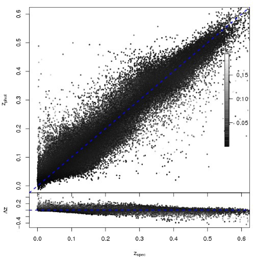
Figure 14: In the upper panel, it is shown the scatterplot of the spectroscopic vs photometric redshifts evaluated with the WGE method for the members of the KB of the experiment for the SDSS galaxies with optical photometry, while in the lower panel the scatterplot of the spectroscopic redshift $z_{\mathrm{spec}}$ vs $\Delta z$ variable is shown for the same sources. All points are color-coded according to the value of the errors $\sigma_{z_{\mathrm{phot}}}$ as evaluated but the WGE.

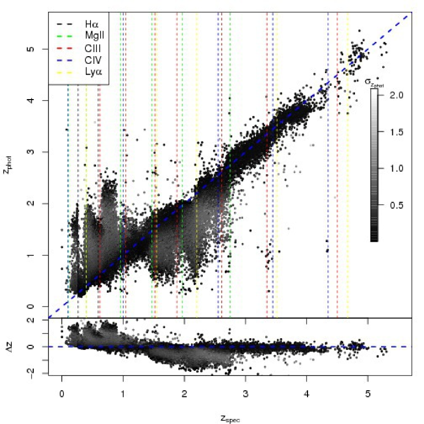
Figure 15: In the upper panel, it is shown the scatterplot of the spectroscopic vs photometric redshifts evaluated with the WGE method for the members of the KB of the experiment for the quasars extracted from the SDSS catalog with optical photometry, while in the lower panel the scatterplot of the spectroscopic redshift $z_{\mathrm{spec}}$ vs $\Delta z$ variable is shown for the same sources. All points are color-coded according to the value of the errors $\sigma_{z_{\mathrm{phot}}}$ as evaluated but the WGE. The vertical dashed lines represent the redshift at which the most luminous emission lines characterizing quasars spectra shift off the SDSS photometric filters due to redshift. Most of the features of the plot are associated to one or more of these lines.

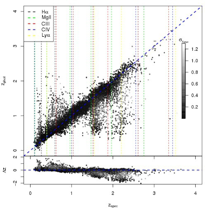
Figure 16: In the upper panel, it is shown the scatterplot of the spectroscopic vs photometric redshifts evaluated with the WGE method for the members of the KB of the experiment for the quasars extracted from the SDSS catalog with optical and ultraviolet photometry, while in the lower panel the scatterplot of the spectroscopic redshift $z_{\mathrm{spec}}$ vs $\Delta z$ variable is shown for the same sources. All points are color-coded according to the value of the errors $\sigma_{z_{\mathrm{phot}}}$ as evaluated but the WGE. The vertical dashed lines represent the redshift at which the most luminous emission lines characterizing quasars spectra shift off the SDSS and GALEX photometric filters due to redshift. Similarly to what is shown in figure 15, most of the features of the plot are associated to one or more of these lines. Moreover, the lines associated to the GALEX filters resolve some of the degeneracies at low redshift.

Table 7: Parameters of the best experiments for the evaluation of the error on the photometric redshifts for optical galaxies, optical candidate quasars and optical plus ultraviolet candidate quasars.

Params. clustering ($\sigma_{z}$)	$\sigma_{u\!-\!g}$,$\sigma_{g\!-\!r}$,$\sigma_{r\!-\!i}$,$\sigma_{i\!-\!z}$	$\sigma_{u\!-\!g}$,$\sigma_{g\!-\!r}$,$\sigma_{r\!-\!i}$,$\sigma_{i\!-\!z}$	$\sigma_{u\!-\!g}$,$\sigma_{g\!-\!r}$,$\sigma_{r\!-\!i}$,$\sigma_{i\!-\!z}$,
	$(u\!-\!g)$,$(g\!-\!r)$,$(r\!-\!i)$,$(i\!-\!z)$,	$(u\!-\!g)$,$(g\!-\!r)$,$(r\!-\!i)$,$(i\!-\!z)$,	$\sigma_{fuv\!-\!nuv}$,$\sigma_{nuv\!-\!u}$,
	$z_{\mathrm{phot}}$,$(z_{\mathrm{phot}}\!-\!z_{\mathrm{spec}})$	$z_{\mathrm{phot}}$,$(z_{\mathrm{phot}}\!-\!z_{\mathrm{spec}})$	$(fuv\!-\!nuv)$,$(nuv\!-\!u)$, $(u\!-\!g)$,$(g\!-\!r)$,
			$(r\!-\!i)$,$(i\!-\!z)$,$z_{\mathrm{phot}}$,$(z_{\mathrm{phot}}\!-\!z_{\mathrm{spec}})$
Min. # clusters ($\sigma_{z}$)	2	2	2
Max. # clusters ($\sigma_{z}$)	9	9	9
Opt. # clusters ($\sigma_{z}$)	2	3	7
Clusters threshold ($\sigma_{z}$)	0.1	0.1	0.1
Max. iterations clust. ($\sigma_{z}$)	500	500	500
Params. experts ($\sigma$)	$\sigma_{u\!-\!g}$,$\sigma_{g\!-\!r}$,$\sigma_{r\!-\!i}$,$\sigma_{i\!-\!z}$	$\sigma_{u\!-\!g}$,$\sigma_{g\!-\!r}$,$\sigma_{r\!-\!i}$,$\sigma_{i\!-\!z}$,	$\sigma_{u\!-\!g}$,$\sigma_{g\!-\!r}$,$\sigma_{r\!-\!i}$,$\sigma_{i\!-\!z}$,
	$(u\!-\!g)$,$(g\!-\!r)$,$(r\!-\!i)$,$(i\!-\!z)$,	$(u\!-\!g)$,$(g\!-\!r)$,$(r\!-\!i)$,$(i\!-\!z)$,	$\sigma_{fuv\!-\!nuv}$,$\sigma_{nuv\!-\!u}$,
	$z_{\mathrm{phot}}$	$z_{\mathrm{phot}}$	$(fuv\!-\!nuv)$,$(nuv\!-\!u)$, $(u\!-\!g)$, $(g\!-\!r)$,
			$(r\!-\!i)$,$(i\!-\!z)$,$z_{\mathrm{phot}}$
Hid. neurons experts ($\sigma_{z}$)	30	20	20
Max. epochs. experts ($\sigma_{z}$)	500	500	500
Learning rate experts ($\sigma_{z}$)	0.01	0.01	0.01
Steepness experts ($\sigma_{z}$)	1.0	1.0	1.0
Hid. neurons gate ($\sigma_{z}$)	30	20	20
Max. epochs. gate ($\sigma_{z}$)	500	500	500
Learning rate gate ($\sigma_{z}$)	0.01	0.01	0.01
Steepness gate ($\sigma_{z}$)	1.0	1.0	1.0
# training gates ($\sigma_{z}$)	20	20	20
MAD ($\sigma$)	0.01	0.086	0.053

The distribution of the errors on the photometric redshifts $\sigma_{z_{\mathrm{phot}}}$ as function of the spectroscopic redshifts, the photometric redshift and the variable $\Delta z$ are shown for the two experiments involving the samples of quasars in the figure 17. As it was to be expected, in general, the WGE produces larger error estimates for the photometric redshifts of the sources lying inside the high degeneracy regions of the $z_{\mathrm{spec}}$ vs $z_{\mathrm{phot}}$ plots. As shown by the vertical dashed lines (upper panels), most of these regions occur at redshifts at which the most luminous emission lines characterizing SDSS quasars spectra shift off the filters of the SDSS or GALEX photometric systems. The shape of the average distribution of the error $\sigma_{z_{\mathrm{phot}}}$ as a function of the variable $\Delta z$, while not globally linear as should have been expected in the case of perfect reconstruction of the errors by the WGE method, is compatible with a linear relation close to the diagonal of the plot for $\Delta z\lesssim 0.3$ for both experiments and represent an acceptable approximation since in this range lies a very high percentage of the total number of sources (from $\sim\!80\%$ to $\sim\!90\%$ of the points).

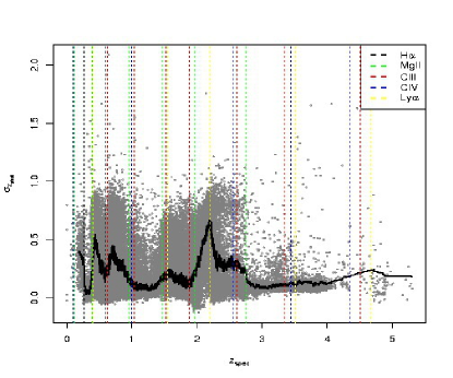
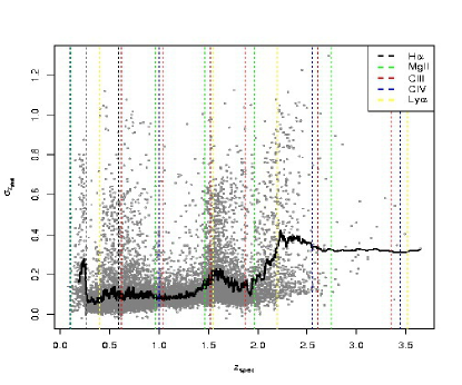
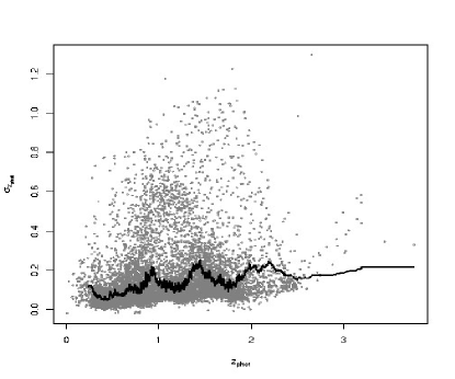
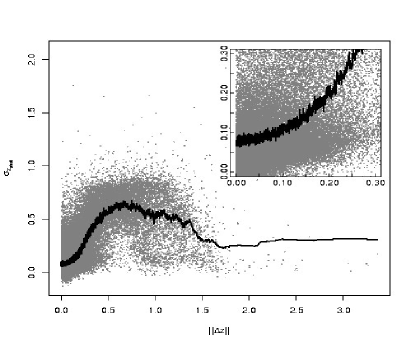
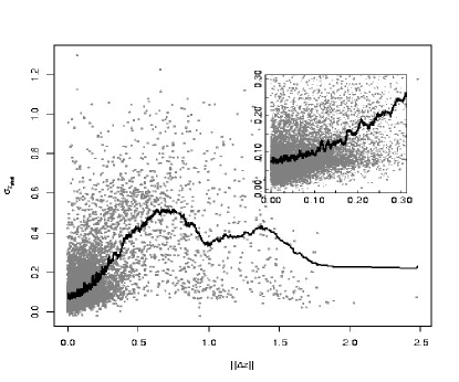
Figure 17: From the upper to the lower plots, the distributions of the errors on the photometric redshifts $\sigma_{z_{\mathrm{phot}}}$ as function of the spectroscopic redshifts $z_{\mathrm{spec}}$, the photometric redshift $z_{\mathrm{phot}}$ and the variable $\|\Delta z\|$ respectively are shown for the two experiments regarding quasars with optical only photometry (left column) and quasars with optical and ultraviolet photometry (right column) discussed in this paper. The average profiles of the distribution of error on the photometric redshifts are shown as a black line in all plots. In the upper plots, the redshifted emission lines are shown similarly to what is done in figures 15 and 16, as lines over-plotted to the $z_{\mathrm{spec}}$ vs $\sigma_{z_{\mathrm{phot}}}$ scatterplots. Also in these cases, most of the features in these two plot can be associated to one or more of the lines. In the lower two plots, the insets show the densest regions of the plots. For the optical quasars (lower left plot), $\sim\!82\%$ of the sample is contained in the inset, while for the optical and ultraviolet quasars (lower right plot), $\sim\!90\%$ of the sample is contained in the zoomed region.

In the case of the reconstruction of the photometric redshifts for the candidate quasars using both the optical or the optical plus ultraviolet photometry, the characterization of the accuracy of the reconstruction of the photometric redshifts provided by the errors is not complete since, similarly to what happens for the $z_{\mathrm{phot}}$ values, the errors on such values are statistical estimates of the real uncertainty and are affected, to some extent, by the same degeneracies and systematic biases found in the $z_{\mathrm{phot}}$ reconstruction. This effect is noticeable in the scatterplots in figures 8 and 10, where consistent features of the plot deviate heavily from the ideal diagonal distribution. The degeneracies yielding such large effects cannot be completely resolved by the WGE during the phase of photometric redshifts estimation, but the same WGE generates information useful to flag the sources located in these regions of the plot (which cannot be recognized exactly in absence of spectroscopic redshifts, i.e. for all the sources belonging to the catalogs of photometric redshifts). For this reason, another measure of the reliability of the redshifts, hereafter called quality flag $q$, is provided for each object belonging to the catalog of photometric redshifts for optical candidate quasars. Unlike the photometric redshift value itself $z_{\mathrm{phot}}$ and the error on such value $\sigma_{z_{\mathrm{phot}}}$, the quality flag $q$ is evaluated on the basis of the global distributions of both photometric redshifts and photometric redshift errors, i.e. after the evaluation of photometric redshifts and of the corresponding errors for all sources in a given sample. The steps for the evaluation of the quality flags are the following:

• The distribution of photometric redshifts evaluated by the WGE for the training set is binned, inside the interval covered by the distribution of spectroscopic redshifts of the KB, in $n_{\mathrm{bin}}(z_{\mathrm{phot}})$ equally spaced intervals;

• For each bin in the distribution of photometric redshifts, the associated set of errors on the estimates of the $z_{\mathrm{phot}}$ is binned in $n_{\mathrm{bin}}(\sigma_{z_{\mathrm{phot}}})$ equally spaced intervals;

• The value of the quality flag of a given photometric redshift $\tilde{z}_{phot}$ is assigned according to the position of its uncertainty relatively to the overall presence of peaked features of the distribution: if the error $\sigma_{\tilde{z}_{\mathrm{phot}}}$ lies inside a bin belonging to the most prominent feature of the histogram (i.e. the component of the histogram containing the highest peak of the overall distribution), the quality flags of the corresponding photometric redshift estimate $q$ is set to 1, otherwise to 0;

• The sources with $q\!=\!1$ are considered reliable, while the sources flagged by $q\!=\!0$ are considered unreliable, i.e. potential catastrophic outliers.

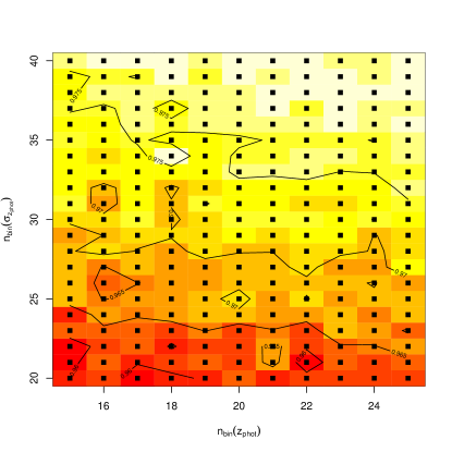
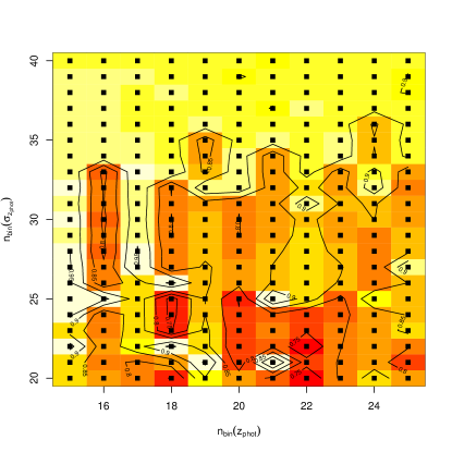
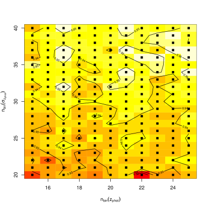
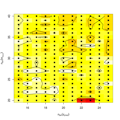
Figure 18: Plots of the efficiency (left column) and of the completeness (right column) of the process of selection of the catastrophic outliers as functions of the two parameters $n_{\mathrm{bin}}(z_{\mathrm{phot}})$ and $n_{\mathrm{bin}}(\sigma_{z_{\mathrm{phot}}})$ involved in the procedure for the determination of the quality flag $q$. The upper plots are associated to the experiment for the evaluation of the photometric redshifts for the optical SDSS quasars, while the lower plots are associated to the third experiment for the estimation of the photometric redshifts of the SDSS quasars with optical and ultraviolet photometry.

The effectiveness of the quality flag in selecting the outliers of the photometric redshifts reconstruction depends critically on the value of the two parameters $n_{\mathrm{bin}}(z_{\mathrm{phot}})$ and $n_{\mathrm{bin}}(\sigma_{z_{\mathrm{phot}}})$ associated to the total number of bins for the photometric redshifts and the error on the photometric redshifts distribution respectively of the process described above. The optimal values of these two parameters have been determined by exploring the $n_{\mathrm{bin}}(z_{\mathrm{phot}})$ vs $n_{\mathrm{bin}}(\sigma_{z_{\mathrm{phot}}})$ space. Two different empirical diagnostics, based on the knowledge of the spectroscopic and photometric redshifts of the sources of the KBs, of the accuracy of the determination of the quality flags have been used, namely the efficiency and the completeness of the separation between reliable sources and unreliable sources. The efficiency $e$ is defined as the ratio of “reliable” sources ($q\!=\!1$) with $\Delta z\!<\!0.3$ to the total number of “reliable” sources ($q\!=\!1$), while the completeness $c$ is defined as the ratio of “reliable” sources ($q\!=\!1$) with $\Delta z\!<\!0.3$ to the total number of sources, independently from the value of the quality flag, with $\Delta z\!<\!0.3$.

The efficiency and completeness for the second and third experiments as functions of the $n_{\mathrm{bin}}(z_{\mathrm{phot}})$ and $n_{\mathrm{bin}}(\sigma_{z_{\mathrm{phot}}})$ parameters are shown in the figures 18. The optimal values of the two parameters $n_{\mathrm{bin}}(z_{\mathrm{phot}})$ and $n_{\mathrm{bin}}(\sigma_{z_{\mathrm{phot}}})$ have been chosen to maximize at the same time the efficiency and completeness, i.e. the product of the efficiency and completeness $t=e\cdot c$, and in the case of equal values, priority has been given to the couple of values associated to the larger efficiency. The optimal values of the parameters for the second experiment, i.e. the determination of the photometric redshifts of the optical SDSS quasars, are $n_{\mathrm{bin}}(z_{\mathrm{phot}})\!=\!18$ and $n_{\mathrm{bin}}(\sigma_{z_{\mathrm{phot}}})\!=\!34$ respectively. For the third experiment, involving the evaluation of the photometric redshifts for SDSS quasars with optical and ultraviolet photometry, the optimal parameters are $n_{\mathrm{bin}}(z_{\mathrm{phot}})\!=\!17$ and $n_{\mathrm{bin}}(\sigma_{z_{\mathrm{phot}}})\!=\!32$. The values of the flags associated to the high redshift quasars $(z_{\mathrm{spec}}\geq 4.5)$ have all been fixed to 1 (reliable photometric redshifts estimates) since, because of low total number of sources in such redshift interval, the method described above for the evaluation of the determination of the outliers based on the overall shape of the binned $z_{\mathrm{phot}}$ distribution in bins of spectroscopic redshifts cannot be applied. The decision to retain all such sources as reliable is based on the eye inspection of the $z_{\mathrm{spec}}$ vs $z_{\mathrm{phot}}$ scatterplot in figure 19.

The scatterplot of the distribution of photometric redshifts as function of the spectroscopic redshifts for the KB associated to the second experiment performed by the WGE (quasars with optical photometry) with different color of the symbol associated to the two different values of the quality flags is shown in figure 19, with marginal histograms of the distribution of the different subsets according to $q$. In order to highlight the differences in the distributions of the sources with reliable or unreliable photometric redshifts values, the $z_{\mathrm{phot}}$ vs $z_{\mathrm{spec}}$ scatterplots for the two samples with $q\!=\!1$ and $q\!=\!0$ respectively are shown in figure 20. These same plots for the experiment concerning the estimation of the photometric redshifts of quasars with optical and ultraviolet photometry, are shown in 21 and 22 respectively. The set of statistical diagnostics calculated for the whole KBs of the three experiments discussed in this paper and shown in table LABEL:table:diagnostics, have been evaluated for the KBs of the second and third experiments separately for sources with $q\!=\!1$ and $q\!=\!0$ (see table 8).

Table 8: Statistical diagnostics of the accuracy of the photometric redshifts reconstruction for the second and third experiments, evaluated for reliable and unreliable $z_{\mathrm{phot}}$ estimates according to the quality flag $q$. For the definition of the statistical diagnostics see section 8.

	Exp. 2			Exp. 3
Diagnostic	All	$q=1$	$q=0$	All	$q=1$	$q=0$
$\left\langle\Delta z\right\rangle$	0.21	0.13	0.53	0.13	0.10	0.52
RMS$(\Delta z)$	0.35	0.24	0.62	0.25	0.20	0.63
$\sigma^{2}(\Delta z)$	0.08	0.04	0.11	0.044	0.031	0.12
MAD$(\Delta z)$	0.11	0.07	0.32	0.061	0.056	0.34
MAD’$(\Delta z)$	$\mathbf{0.098}$	$\mathbf{0.064}$	$\mathbf{0.41}$	$\mathbf{0.062}$	$\mathbf{0.047}$	$\mathbf{0.29}$
$\%(\Delta z_{1})$	50.7	61.9	5.9	68.1	71.4	8.5
$\%(\Delta z_{2})$	72.3	86.6	15.2	86.5	90.4	18.2
$\%(\Delta z_{3})$	80.5	90.6	27.5	91.4	95.0	28.6
$\sigma^{2}(\Delta z_{1})$	$7.9\!\cdot\!10^{-4}$	$7.9\!\cdot\!10^{-4}$	$8.3\!\cdot\!10^{-4}$	$7.6\!\cdot\!10^{-4}$	$7.6\!\cdot\!10^{-4}$	$8.4\!\cdot\!10^{-4}$
$\sigma^{2}(\Delta z_{2})$	0.003	0.003	0.003	0.023	0.002	0.003
$\sigma^{2}(\Delta z_{3})$	0.005	0.004	0.007	0.039	0.004	0.007
$\left\langle\Delta z_{\mathrm{norm}}\right\rangle$	0.095	0.056	0.25	0.058	0.049	0.23
RMS$(\Delta_{\mathrm{norm}})$	0.19	0.13	0.32	0.11	0.09	0.29
$\sigma^{2}(\Delta z_{\mathrm{norm}})$	0.025	0.014	0.036	0.086	0.006	0.03
MAD$(\Delta z_{\mathrm{norm}})$	0.041	0.028	0.14	0.029	0.027	0.16
MAD’$(\Delta z_{\mathrm{norm}})$	$\mathbf{0.04}$	$\mathbf{0.030}$	$\mathbf{0.19}$	$\mathbf{0.031}$	$\mathbf{0.029}$	$\mathbf{0.204}$
$\%(\Delta z_{\mathrm{norm},1})$	77.3	92.2	17.5	87.4	91.0	23.3
$\%(\Delta z_{\mathrm{norm},2})$	87.3	96.8	49.3	94.0	96.6	49.1
$\%(\Delta z_{\mathrm{norm},3})$	91.8	97.1	70.3	96.4	97.8	71.2
$\sigma^{2}(\Delta z_{\mathrm{norm},1})$	$6.2\!\cdot\!10^{-4}$	$5.7\!\cdot\!10^{-4}$	$8.4\!\cdot\!10^{-4}$	$5.6\!\cdot\!10^{-4}$	$5.5\!\cdot\!10^{-4}$	$8.2\!\cdot\!10^{-4}$
$\sigma^{2}(\Delta z_{\mathrm{norm},2})$	0.002	$9.8\!\cdot\!10^{-4}$	0.003	0.001	0.001	0.003
$\sigma^{2}(\Delta z_{\mathrm{norm},3})$	0.004	0.001	0.006	0.002	0.002	0.007

The accuracy of the reconstruction of the photometric redshifts for the reliable sources ($q=1$) increases with a factor from 1.2 to 2 in terms of both the variables RMS($\Delta z$) and MAD($\Delta z$) for both experiments involving the determination of the photometric redshifts of quasars. While a significant contamination from photometric redshifts with $\|\Delta z\|>0.1$ is still present in the subsets of reliable sources in both experiments ($\%(\|\Delta z\|<0.1)=61.9$ and 71.4 for Exp. 2 and Exp. 3 respectively), the fraction of accurate $z_{\mathrm{phot}}$ ($\|\Delta z\|<0.1$) selected as unreliable ($q=0$) at the $\|\Delta z\|=0.1$ level is very low ($5.9\%$ and $8.5\%$ respectively).

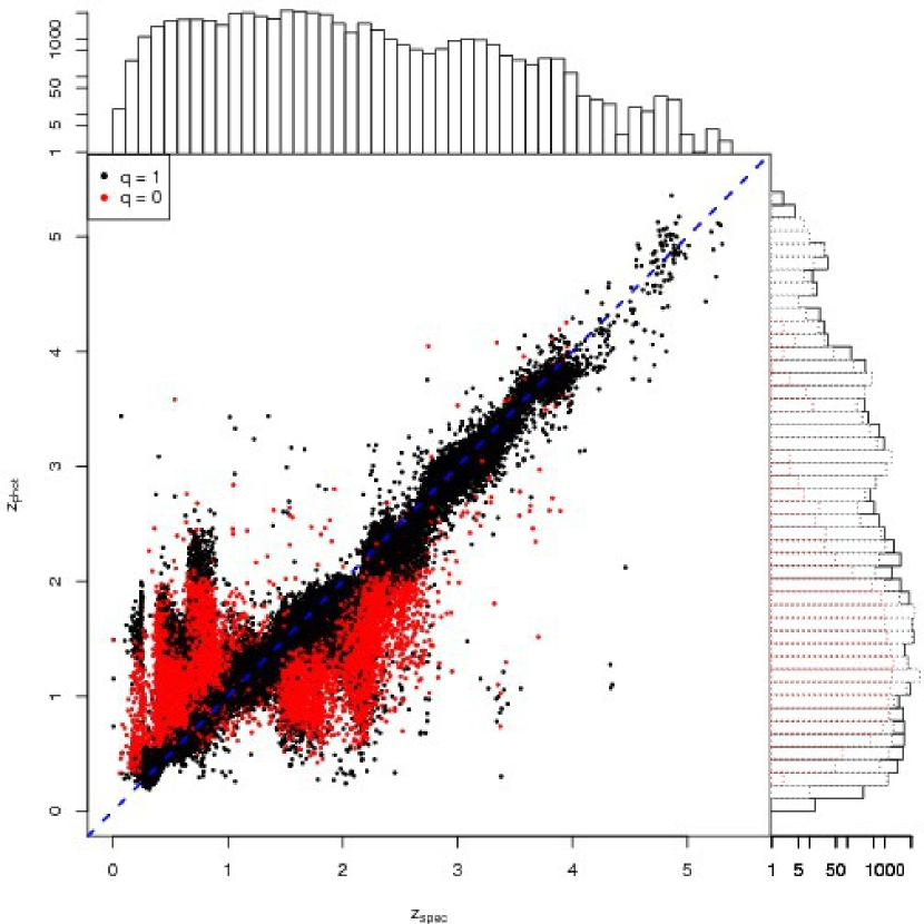
Figure 19: Scatterplot of the spectroscopic vs photometric redshifts for the KB of the second experiment (quasars with optical photometry), with marginal histograms for reliable ($q\!=\!1$) and unreliable ($q\!=\!0$) photometric redshift estimates according to the quality flag $q$. In the vertical marginal panel, the histograms of the distributions of reliable and unreliable photometric redshifts are respectively plotted with black and red dotted lines, while the histogram of the spectroscopic redshifts distribution is shown as a solid black line in both marginal panels.

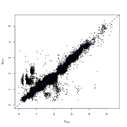
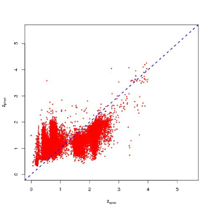
Figure 20: Scatterplots of the spectroscopic vs photometric redshifts distributions for the KB of the second experiment (quasars with optical photometry) separately for reliable and unreliable estimations of the photometric redshifts according to the quality flag $q$. The sources with reliable $z_{\mathrm{phot}}$ values ($q\!=\!1$) are shown in the plot on the left, while sources with unreliable $z_{\mathrm{phot}}$ values ($q\!=\!0$) are shown in the plot on the right.

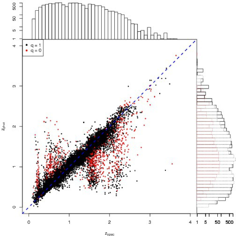
Figure 21: Scatterplot of the spectroscopic vs photometric redshifts for the KB of the third experiment (quasars with optical and ultraviolet photometry), with marginal histograms for reliable and unreliable photometric redshift estimates according to the quality flag $q$. In the vertical marginal panel, the histograms of the distributions of reliable and unreliable photometric redshifts are respectively plotted with black and red dotted lines, while the histogram of the spectroscopic redshifts distribution is shown as a solid black line in both marginal panels.

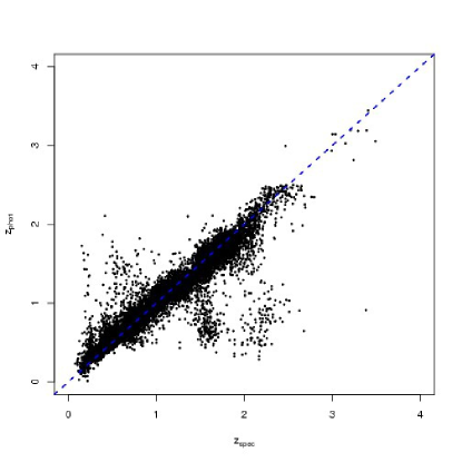
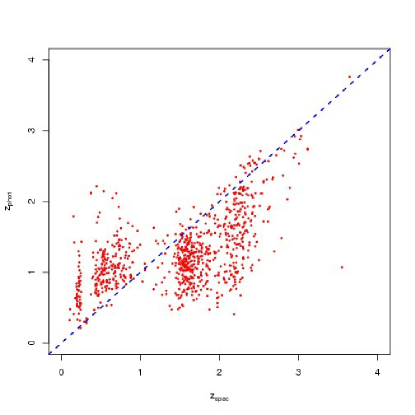
Figure 22: Scatterplots of the spectroscopic vs photometric redshifts distributions for the KB of the third experiment (quasars with optical and ultraviolet photometry) separately for reliable and unreliable estimations of the photometric redshifts according to the quality flag $q$. The sources with reliable $z_{\mathrm{phot}}$ values ($q\!=\!1$) are shown in the plot on the left, while sources with unreliable $z_{\mathrm{phot}}$ values ($q\!=\!0$) are shown in the plot on the right.

10 Conclusions

The Weak Gated Expert or WGE is an original method for the determination of the photometric redshifts capable of working on both galaxies and quasars. The WGE, which is based on a combination of clustering and regression techniques, is able to mitigate most of the degeneracies which arise from the distribution of KB templates in the features space, and to derive accurate estimates of both the photometric redshifts values and of their errors. Besides giving a detailed description of how the WGE works, in this paper we have also presented an application of the WGE to the determination of photometric redshifts of optical galaxies and to the candidate quasars with optical and ultraviolet photometry, both extracted from the SDSS-DR7 database. The accuracy of the reconstruction of the redshifts for optical galaxies, obtained by comparing photometric and spectroscopic redshifts, can be expressed a robust estimate of the dispersion of the $\Delta z$ variable, which is equal to MAD($\Delta z$) = 0.011 with $\sim 86.9\%$ of the sources within $\Delta z_{3}$. The same diagnostics for the estimation of $z_{\mathrm{phot}}$ for candidate quasars are MAD($\Delta z$) = 0.11 and $\%(\Delta z_{3})=80.5$ when only optical photometry is used, reaching MAD($\Delta z$) = 0.061 and $\%(\Delta z_{3})=91.4$ when the photometric redshifts are evaluated using both optical and ultraviolet photometry. A thorough discussion and a comparison of the WGE with several other methods applied to the same or similar data is also provided in the paper. To perform such comparison, a large set of statistical diagnostics shows that the WGE performs better than or similarly to all the other methods. The results of the best experiments with the WGE for optical galaxies and quasars have been used to produce the catalogs of photometric redshifts of $\sim 3.2\!\cdot\!10^{7}$ galaxies photometrically selected, a sample of $\sim 2.1\!\cdot\!10^{6}$ optical candidate quasars from [D’Abrusco et al. 2009] with photometric redshifts estimated using optical only photometry and a smaller catalog of more accurate photometric redshifts derived from optical and ultraviolet photometry for a subset of $\sim 1.6\!\cdot\!10^{5}$ optical candidate quasars respectively. All catalogs will be publicly available and a complete description of the parameters associated to each photometric redshift estimates is available (see 7.1, 7.2 and 7.3 respectively for details on the catalogs). In this paper, we have also shown the results of the application of the WGE method to a relatively small sample of spectroscopically selected optical SDSS quasars for which also the ultraviolet (GALEX) photometry was available. Since the largest computational load is in the training phase, once the WGE has been trained and has has achieved the required accuracy (either by matching some a priori constraint or by convergence), it can be “frozen” and newly acquired data falling in the same region of the features space sampled by the KB can be processed without the need for a re-training of the method. This implies that, regardless the rate at which data are acquired, the WGE can produce estimates of photometric redshifts in real-time. If needed, a new training of the method can be performed off-line when a larger/improved KB becomes available. This requirement is becoming of the utmost importance for data mining techniques in order for them to cope with the data streams foreseen for the current and future optical synoptic surveys (such as Pan-STARRS or the LSST) that will produce overnight an amount of data (images and catalog) similar or even larger than the total amount of data collected by the SDSS. It is worth stressing that the WGE is part of the larger realms of Astroinformatics and Data Mining. As a data-driven discipline, through the application of Data Mining methods, Astroinformatics can provide Astronomy and Astrophysics with a framework for tackling new problems or old problems with a novel approach: in particular, where the traditional approach uses data from observations in order to prove or disprove an hypothesis, with Data Mining we want data itself to provide hypotheses that can be then proved or disproved with more accurate follow-up observation. For example, using a catalog of photometric redshifts for galaxies of the SDSS DR7 survey, [Capozzi et al. 2009] put constraints on the nature of the so called Shakbazian groups by studying the properties of such groups as they appeared to be in the de-projected space. This data-driven approach is well described also by the fact that by using machine learning methods many assumptions can be dropped in favor of a more agnostic approach: for instance, by employing machine learning techniques to the photometric redshift problem, one can drop any assumptions on the form of the SED of the source, so that it is up to the model, for example a neural network, to find a representation of the highly non-linear relation between the photometric information and the spectroscopic redshift, instead of fitting the data with a set of SED templates. However, since the hypothesis driven approach of template fitting has noticeable advantages, it can be useful to underline an interesting feature offered by the WGE: it is possible, through the WGE, to link together different experts employed in complex architectures, in which different predictors can be integrated to take advantage of the peculiar strengths of each of them. Even an algorithm which does not belong to the domain of the DM techniques could be consistently used together with machine learning experts. In this case, however, the predictors not based on DM techniques will not be trained in the first step of the training algorithm and will only participate to the training of the gate predictor. This feature was not exploited in this work, but a likely outcome of such a hybrid approach will be the creation of mixed WGE architectures in which empirical machine learning algorithms cooperate with more traditional algorithms based on physical knowledge, for instance neural networks and SED template fitting

One interesting feature of this approach is the generalization offered by the WGE: linking together different experts can lead to complex architectures in which different predictors can be integrated to take advantage of the peculiar strengths of each of them. Even an algorithm which does not belong to the domain of the DM techniques can be consistently used together with machine learning experts. In this case, however, the predictors not based on DM techniques will not be trained in the first step of the training algorithm and will only participate to the training of the gate predictor. A likely outcome of such hybrid approach will be the creation of mixed WGE architectures in which empirical machine learning algorithms cooperate with more classical algorithms based on physical consideration or models typical of the specific domain. For instance, for the particular problem of the estimation of photometric redshifts, the WGE method could be used to integrate machine learning algorithms and the empirical methods based on SED template fitting (for a review of the most used template fitting methods in the literature see [Hildebrandt et al. 2010]).

Appendix A SQL query for SDSS galaxies

This is an example of the SQL queries used to retrieve the galaxies in the SDSS photometric dataset whose redshifts have been evaluated using the results of the WGE experiment described in 7.1. The queries were run on the DR7 SDSS database through the SDSS Catalog Archive Server Jobs System (CASJobs).

SELECT

g.objID,
g.ra, g.dec,
g.dered_u, g.dered_g ,g.dered_r, g.dered_i, g.dered_z,
g.modelmagerr_u, g.modelmagerr_g, g.modelmagerr_r,
g.modelmagerr_i, g.modelmagerr_z,
g.extinction_u, g.extinction_g, g.extinction_r, g.extinction_i,
g.extinction_z,
g.petroR50_u,g.petroR90_u,
g.petroR50_g,g.petroR90_g,
g.petroR50_r,g.petroR90_r,
g.petroR50_i,g.petroR90_i,
g.petroR50_z,g.petroR90_z,
g.lnLDeV_u,g.lnLDeV_r,
g.lnLExp_u,g.lnLExp_r,
g.lnLStar_u,g.lnLStar_r

FROM

Galaxy AS g, Segment AS seg, Field AS f

WHERE

g.mode = 1 AND
seg.segmentID = f.segmentID AND
f.fieldID = g.fieldID AND
seg.stripe = 16 AND
g.dered_r < 21.5 AND
dbo.fPhotoFlags(’PEAKCENTER’) != 0 AND
dbo.fPhotoFlags(’NOTCHECKED’) != 0 AND
dbo.fPhotoFlags(’DEBLEND_NOPEAK’) != 0 AND
dbo.fPhotoFlags(’PSF_FLUX_INTERP’) != 0 AND
dbo.fPhotoFlags(’BAD_COUNTS_ERROR’) != 0 AND
dbo.fPhotoFlags(’INTERP_CENTER’) != 0

Appendix B SQL query for optical SDSS stellar sources

This is an example of the SQL queries used to retrieve the stellar sources in the SDSS photometric dataset from which the candidate quasars have been extracted with the method described in 7.2.1 and the photometric redshifts have been evaluated using the results of the WGE experiment described in 7.2. The queries were run on the DR7 SDSS database through the SDSS Catalog Archive Server Jobs System (CASJobs).

SELECT

p.objID,
p.ra, p.dec,
p.psfMag_u, p.psfMag_g, p.psfMag_r, p.psfMag_i,p.psfMag_z,
p.psfmagerr_u,p.psfmagerr_g,p.psfmagerr_r,
p.psfmagerr_i,p.psfmagerr_z,
p.extinction_u,p.extinction_g,p.extinction_r,
p.extinction_i, p.extinction_z

FROM

PhotoObjAll AS p, Segment AS seg, Field AS f

WHERE

p.mode = 1 AND
p.type = 6 AND
seg.segmentID = f.segmentID AND
f.fieldID = p.fieldID AND
seg.stripe = 11 AND
p.psfmag_i > 14.5 AND
(p.psfMag_i - p.extinction_i) < 21.3 AND
p.psfmagErr_i < 0.2 AND
dbo.fPhotoFlags(’PEAKCENTER’) != 0 AND
dbo.fPhotoFlags(’NOTCHECKED’) != 0 AND
dbo.fPhotoFlags(’DEBLEND_NOPEAK’) != 0 AND
dbo.fPhotoFlags(’PSF_FLUX_INTERP’) != 0 AND
dbo.fPhotoFlags(’BAD_COUNTS_ERROR’) != 0 AND
dbo.fPhotoFlags(’INTERP_CENTER’) != 0

Appendix C SQL query for ultraviolet GALEX counterparts of optical candidate quasars

This is an example of the SQL queries used to retrieve the ultraviolet GALEX counterparts of the optical candidate quasars composing the catalog described in 7.3, whose photometric redshifts have been evaluated using the results of the WGE experiment described in 6.3.

SELECT

p.objid AS galex$\_$objid,
my.objID AS sdss$\_$objid,
p.nuv$\_$mag as nuv, p.nuv$\_$magErr as nuv$\_$err,
p.fuv$\_$mag as fuv, p.fuv$\_$magErr as fuv$\_$err,
p.e$\_$bv,
x.distance,
x.distanceRank,
x.reverseDistanceRank,
x.multipleMatchCount,
x.reverseMultipleMatchCount

FROM

MYDB.candidate$\_$quasars$\_$objid AS my
INNER JOIN xSDSSDR7 AS x ON my.objID = x.SDSSobjid
INNER JOIN photoobjall AS p ON x.objid = p.objid

WHERE

x.distanceRank = 1
AND x.reverseDistanceRank = 1
AND x.distance < 2
AND p.nuv$\_$mag > 0
AND p.fuv$\_$mag > 0

References

- [Abazajian et al. 2009] Abazajian, K. N. et al. 2009, ApJS, 182, 2, 543-558
- [Abdalla et al. 2009] Abdalla, F. B. et al. 2009, MNRAS, 387, 969-986
- [Arnalte-Mur et al. 2009] Arnalte-Mur, P. et al. 2009, MNRAS, 394, 1631
- [Ball et al. 2008] Ball, N. M. et al. 2008, ApJ, 683, 1, 12-21
- [Ball & Brunner 2010] Ball, N. M. & Brunner, R. J. 2010, IJMPD, 99, issue 07, 1049-1106
- [Bishop 1996] Bishop, C. M. 1996, Neural networks for pattern recognition, Oxford University Press, Oxford, UK, 1996.
- [Bonfield et al. 2010] Bonfield, D. G. et al. 2010, MNRAS, 405, 987
- [Borne 2009] Borne, K. 2009, Astroinformatics: a 21st century approach to astronomy, in Astro2010 Decadal Survey State of the Profession Position Paper
- [Brescia et al. 2010] Brescia, M. et al. 2010, submitted to the Journal of Computing Science
- [Bruzual 2010] Bruzual, A. G. 2010, in Proceedings of the International Astronomical Union, 262, 55-64
- [Budavari et al. 2001] Budavari, T. et al. 2001, AJ, 120, 1588
- [Budavari et al. 2009] Budavari, T. et al. 2009, ApJ, 394, 1281-1292
- [Capozzi et al. 2009] Capozzi, D. et al. 2009, MNRAS, 396, 2, 900-917
- [Carliles et al. 2010] Carliles, S. et al. 2010, ApJ, 712, 511
- [Collister & Lahav 2004] Collister, A. A. & Lahav, O. 2004, PASP, 116, 345
- [Collister et al. 2007] Collister, A. A., Lahav, O., Blake, C., 2007, MNRAS, 375, 68
- [Connolly et al. 1995] Connolly, A. J. et al. 1995, AJ, 110, 2655
- [Croom et al. 2004] Croom, S. M. et al. 2004, MNRAS, 349, 1397
- [Csabai et al. 2003] Csabai, I., et al. 2003, AJ, 125, 580
- [D’Abrusco et al. 2007] D’Abrusco, R. et al. 2007, ApJ, 632, 752
- [D’Abrusco et al. 2009] D’Abrusco, R. et al. 2009, MNRAS, 1, 223-262
- [Davis et al. 2007] Davis, M. et al. 2007, ApJ, 660, 1, L1-L6
- [Dunn 1973] Dunn, J. C. 1973, Journal of Cybernetics, 3, 32-57
- [Firth et al. 2003] Firth, A. E., Lahav, O. & Somerville, R. S. 2003, MNRAS, 339, 1195
- [Freeman et al. 2009] Freeman, P. E., et al. 2009, 398, 2012-2021
- [Fukugita et al. 1996] Fukugita, N. 1996, AJ, 111, 1748
- [Gerdes et al. 2010] Gerdes, D. W. et al. 2010, ApJ, 715, 823
- [Hey et al. 2009] Hey, T. et al. editors, The Fourth Paradigm: data intensive scientific discovery, Microsoft Research, available at http://research.microsoft.com/en-us/collaboration/fourthparadigm/
- [Hildebrandt et al. 2010] Hildebrandt, H. et al. 2010, AA, in press
- [Jordan & Jacobs 1994] Jordan, I. M. & Jacobs, R. .A. 1994, Neural Computation, 6(2):181214
- [Krogh & Vedelsby 1995] Krogh, A. & Vedelsby, J. 1995, Neural network ensembles, cross validation and active learning, in Advances in Neural Information Processing Systems, 231 238, MIT Press.
- [Li et al. 2008] Li, I. H. & Yee, H. K. C. 2008, AJ, 135, 809
- [Quadri & Williams 2010] Quadri, R. F. & Williams, J. 2010, ApJ, 725, 794
- [Richards et al. 2009] Richards, G. T. et al. 2009, ApJS, 180, 67-83
- [Salvato et al. 2009] Salvato, M. et al. 2009, ApJ, 690, 2, 1250-1263
- [Schlegel et al. 1998] Schlegel, D. et al. 1998, in Proceedings of the 14th IAP meeting
- [Stoughton et al. 2002] Stoughton, C. et al. 2002, AJ, 123, 485-548
- [Subbarao et al. 1996] Subbarao, M. U., Connolly, A. J., Szalay, A. S. & Koo, D.C., 1996, AJ, 112, 929
- [Taylor 2005] Taylor, M. B. 2005, ADASS Conference Series, 347, 29
- [Taylor 2006] Taylor, M. B. 2006, ADASS Conference Series, 351, 666
- [Tresp et al. 1994] Tresp, V. et al. (1994), in Advances in Neural Information Processing Systems, volume 6, pp 128-135
- [Vanzella et al. 2004] Vanzella, E. et al. 2004, A&A, 423, 761
- [Wadadekar 2005] Wadadekar, Y. 2005, PASP, 117, 79
- [Way & Srivastava 2006] Way, M. J. & Srivastava, A. N. 2006, ApJ, 647, 102
- [Weigend et al. 1995] Weigend, A. S. 1995, International Journal of Neural Systems, 6, 373-399
- [Wu & Jia 2010] Wu, X.B & Jia, Z. 2010, MNRAS, 406, 1583
- [Yèche et al. 2010] Yèche, C. et al. A&A, 523, 14Y