An MCMC approach to extracting the global 21-cm signal during the cosmic dawn from sky-averaged radio observations

Abstract

Efforts are being made to observe the 21-cm signal from the ‘cosmic dawn’ using sky-averaged observations with individual radio dipoles. In this paper, we develop a model of the observations accounting for the 21-cm signal, foregrounds, and several major instrumental effects. Given this model, we apply Markov Chain Monte Carlo techniques to demonstrate the ability of these instruments to separate the 21-cm signal from foregrounds and quantify their ability to constrain properties of the first galaxies. For concreteness, we investigate observations between 40 and 120 MHz with the proposed DARE mission in lunar orbit, showing its potential for science return.

1 Introduction

One of the remaining frontiers of modern cosmology is the end of the ‘dark ages’ and the ‘cosmic dawn’. This is the period ranging from roughly 100 million years ($z\sim 30$) to a billion years ($z\sim 6$) after the Big Bang, when the first stars and galaxies formed, lighting up the Universe. This period lies at the edge of current observational techniques and is of considerable theoretical interest. The next decade is expected to see significant improvements in observations as telescopes such as the James Webb Space Telescope (JWST) and the Atacama Large Millimeter Array (ALMA) go online. These instruments will provide considerable information about galaxy formation at $z\lesssim 10$–$15$, but even these large telescopes will be hard pressed to probe the very beginning of the cosmic dawn.

Measurements of 21-cm emission and absorption from intergalactic hydrogen at high redshift promise to increase greatly our knowledge of the Universe at redshifts $z\gtrsim 6$ (Madau, Meiksin & Rees, 1997). Experiments under way at present are concentrating on frequencies $\nu\gtrsim 100\ \mathrm{MHz}$ ($z\lesssim 13.2$), and are hoping to capture the transition from an almost completely neutral Universe to an almost completely ionized one (the epoch of reionization, or EoR). Future observations at yet lower frequencies (higher redshifts) may probe the epoch when the first sources formed – ‘cosmic dawn’ – and even the preceding ‘dark ages’.

There are two main approaches to making these measurements: using a large interferometric array to produce statistics (e.g. power spectra), and perhaps even images, of the 21-cm brightness temperature; or using a single antenna to measure the mean brightness temperature as a function of frequency and redshift (Shaver et al., 1999). In either case, the bright foregrounds at low frequencies present one of the most significant challenges to extracting the 21-cm signal. The difficulty is alleviated somewhat in the former approach since an interferometer is sensitive only to fluctuations in the foregrounds, which are small compared to the mean on the scales of interest, but they still exceed the 21-cm fluctuations in intensity by several orders of magnitude. Interferometric measurements have other benefits too. For example, the spectrum of fluctuations carries more information than the mean signal alone, and interferometers may make it easier to identify and excise man-made radio-frequency interference (RFI). An interferometer cannot measure the mean signal, however. Moreover, global signal experiments designed to measure the mean brightness temperature may be much simpler and cheaper than large arrays, and are not troubled to the same extent by distortions caused by the Earth’s ionosphere.

The large sky temperature at these frequencies also means that the sky makes the dominant contribution to the system temperature, and hence to the sensitivity of the observation for a given bandwidth and integration time. The brightness temperature, $T_{\mathrm{B}}$, of the diffuse foregrounds depends on the observing frequency, $\nu$, as $T_{\mathrm{B}}\sim\nu^{-2.5}$ (Rogers & Bowman, 2008), so interferometric measurements during the cosmic dawn at less than 100 MHz require very long integration times or arrays with a very large collecting area. Because ionospheric effects also become more serious at low frequencies, it has been suggested that the far side of the Moon, which is also free (as yet) from RFI, would be the best and perhaps the only site for an array to probe the cosmic dawn and dark ages (e.g. Burns & Mendell, 1988; Burns, 2009; Jester & Falcke, 2009). Building and operating such an array of the requisite size would be quite a formidable undertaking, so global signal experiments provide the best hope for probing the 21-cm signal at $z\gtrsim 15$ in the near future.

The EDGES experiment (Bowman & Rogers, 2010), operating at 100–200 MHz, has pioneered global 21-cm measurements, recently placing limits on how rapidly the global 21-cm signal may vary with frequency, and thereby putting a lower limit on the duration of the reionization epoch. Even from its superb radio-quiet site in Western Australia, however, it encountered RFI from sources such as telecommunications satellites and radio and television transmitters. The signals from these may reach EDGES quite directly, or arrive via e.g. tropospheric scattering or reflections from aircraft and meteor trails. This requires a large fraction of the data to be discarded, which would be more damaging at low frequencies where longer integrations are required, and it imposes stringent demands on the dynamic range of the receiver.

A dipole antenna in orbit around the Moon could avoid these problems, since it would be free of RFI when shielded from the Earth over the lunar farside. In addition, an antenna in space experiences a simpler and more stable environment than one on the Earth’s surface, which may allow for more straightforward calibration. The use of lunar orbit does not require anything to be landed on the Moon’s surface, unlike for a farside array. Such a mission concept has been developed, called the Dark Ages Radio Explorer (DARE; Burns et al., 2011). In this paper we therefore explore the constraints that a mission such as DARE could place on a model of the 21-cm brightness temperature between the end of the cosmic dark ages and the start of the epoch of reionization. We aim to include all the most important contributions to the low-frequency radio spectra measured by a dipole in lunar orbit: the redshifted 21-cm signal itself; spatially varying diffuse foregrounds based on an empirical model of the low-frequency radio sky; the Sun; the thermal emission of the Moon; the reflection of emission from other sources by the Moon; the response of the instrument, which is based on an electromagnetic model of an antenna design proposed for the DARE mission; and the thermal noise for a realistic mission duration. Parameters describing all these components must be fit simultaneously from the data since, for example, it may be that the properties of the instrument cannot be computed or measured on the ground with sufficient accuracy to allow recovery of the 21-cm signal in the presence of the very bright foregrounds.

We therefore extend the work of Pritchard & Loeb (2010), who used Fisher matrix and Monte Carlo methods to predict the accuracy with which models of the 21-cm signal could be constrained by a single antenna, but who considered the simpler case of an experiment which measured a single, deep spectrum (i.e. they did not consider the variation of foregrounds over the sky), and where the only contributions to the measured spectrum were the redshifted 21-cm signal, diffuse foregrounds and noise.

The techniques that we develop, and the basic form of our model for the 21-cm global signal, are quite generic and may be applied to future experiments both on the ground and in space. For concreteness, we focus here on the proposed DARE mission, but a similar methodology could be applied to EDGES and other ground based experiments. We plan to investigate this in the near future.

We start by outlining the relevant features of our reference experiment, a proposed mission to measure the 21-cm global signal from lunar orbit, in Section 2. Then, in Section 3 we describe all the different effects which are included in our simulations of data from such a mission, including the parametrizations we use. We also discuss some other contributions, such as impacts of exospheric dust on the antenna and radio recombination lines, and justify neglecting them in this analysis.

Constraints on the model parameters are derived using a Markov Chain Monte Carlo (MCMC) method. In Section 4 we introduce our implementation of this technique and, as an example, show how well the parameters are recovered by a perfect instrument, which is sensitive across the whole frequency band and whose properties are known exactly. In Section 5 we consider a more realistic instrument with an imperfectly known response, and look at the impact of the various processes we model on the quality of our constraints. Finally, we offer some conclusions in Section 6.

2 Reference experiment

We base our simulations on the proposed DARE mission, a fuller description of which will be given by Burns et al. (2011), and which acts as our reference experiment. DARE is designed to carry a low-frequency radio antenna in a circular, equatorial orbit 200 km above the surface of the Moon. Data would only be taken during the part of the orbit when the Moon blocks RFI from the Earth. Approximately 30 min out of each 127 min orbit is spent out of direct line of sight of the Earth and outside the diffraction zone of terrestrial RFI around the lunar limb. A conservative estimate for the total amount of useful integration time for a mission duration of three years is 3000 h.

The primary data product will be a series of spectra at 40–120 MHz with an integration time of 1 s, and with a spectral resolution of around 10 kHz. The analysis in this paper assumes that these spectra have been combined into spectra with a resolution of 2 MHz in a number of discrete sky regions. This could be done either by taking discrete pointings in different directions, and integrating for a long time in each direction, or by scanning the pointing direction across the sky and performing a map-making procedure to combine the individual spectra together. In this paper we simulate only the final, integrated spectra, not the individual high-resolution spectra or the process of combining them.

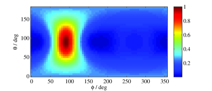
Figure 1: The simulated power pattern of one of the pair of dipoles which constitutes the DARE antenna at 75 MHz, plotted as a function of angle on the sky. The response is normalized to unity at its maximum, and the coordinate system is chosen such that the antenna points towards the positive y-axis ($\theta=\phi=90^{\circ}$). The pattern appears stretched in the $\theta$ direction, but the combined pattern with the other dipole oriented at right-angles to the first is more symmetric.

The antenna consists of a pair of tapered, biconical, electrically short dipoles, designed by R. Bradley of NRAO to satisfy the requirements of the DARE mission (Burns et al., 2011). To increase the directivity, a form of ground plane is provided by radials extending out from the main body of the spacecraft. The design provides a beam with a single primary lobe with a half-power beam area of around 1–2 sr, depending on frequency (the full width at half maximum of the power pattern at 75 MHz is $57\degr$), so that at any one time the antenna is sensitive to radiation from a large fraction of the sky. Despite the radials, the antenna has some sensitivity to radiation from behind the spacecraft (a backlobe, diminished by 9–15 dB). The simulated power response of one of the dipoles as a function of angle at 75 MHz is shown in Fig. 1. The model used to predict this pattern incorporates the design of the antennas themselves and their support structures, the radials which form the ‘ground screen’, and the spacecraft structure itself.

The antenna and the receiver are designed to produce a smooth frequency response. The primary method by which the foregrounds are distinguished from the 21-cm signal is through the spectral smoothness of the foregrounds, so it is essential that the receiving system does not compromise this smoothness. The frequency response of the system has been modelled, and is discussed further in Section 3.4.

3 Simulations of mission data

An overview of some of the different contributions to a spectrum measured by low-frequency radio antenna in lunar orbit is given in Fig. 2. Even when the antenna is oriented such that it is sensitive mainly to an area of sky away from the Galactic centre, the diffuse foregrounds (which consist mainly of synchrotron radiation from our own Galaxy, with some contribution from free-free emission and extragalactic sources; see e.g. Shaver et al. 1999) are between four and six orders of magnitude brighter than the 21-cm signal. Indeed, there are several other contributions which dominate the 21-cm signal. In this section we describe our models for all these contributions, and how they are combined into a simulation of the data returned by a lunar-orbiting dipole experiment.

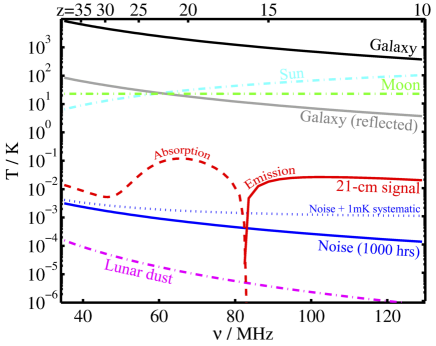
Figure 2: A comparison of the intensity of the 21-cm signal with that of various foregrounds and the thermal noise, as a function of frequency (bottom axis) and the corresponding redshift of the 21-cm line (top axis). From the top (as they appear on the right-hand side of the plot), the different lines show spectra of: 1) The diffuse foregrounds, from a region of sky away from the Galactic centre (solid black line); 2) The quiet Sun (dot-dashed cyan line); 3) The Moon, attenuated by being seen only through the backlobe of our simulated antenna (dot-dashed green line); 4) The diffuse foregrounds reflected by the Moon and entering the backlobe of the antenna (solid grey line); 5) The 21-cm signal (solid red line in emission, dashed red line in absorption); 6) & 7) Thermal noise after 1000 hours (solid blue line), and this noise with the addition of a 1mK systematic residual (dotted blue line); 8) Radio emission caused by the impact of dust particles from the lunar exosphere on the spacecraft and antenna (dot-dashed magenta line).

3.1 The 21-cm signal

The physics behind the properties of redshifted 21-cm emission and absorption was reviewed by Furlanetto, Oh & Briggs (2006), and the evolution of the 21-cm signal with redshift (or cosmic time) was studied in more detail by Madau et al. (1997); Ciardi & Madau (2003); Furlanetto (2006); Pritchard & Loeb (2008). Of most interest here is the redshift evolution of the sky-averaged (‘global’) signal. More precisely, we look at the brightness temperature difference, $\delta T_{\mathrm{b}}$, between 21-cm signal and the CMB at the emission or absorption redshift, where $\delta T_{\mathrm{b}}<0$ indicates absorption against the CMB and $\delta T_{\mathrm{b}}>0$ indicates emission. This is given by

$$\begin{split}\delta T_{\mathrm{b}}&=27x_{\mathrm{HI}}\left(\frac{T_{\mathrm{S}}-T_{\gamma}}{T_{\mathrm{S}}}\right)\left(\frac{1+z}{10}\right)^{\frac{1}{2}}\\ &\quad\times(1+\delta_{\mathrm{b}})\left[\frac{\partial_{r}v_{r}}{(1+z)H(z)}\right]^{-1}\,\mathrm{mK}\ ,\end{split}$$ (1)

where $x_{\mathrm{HI}}$ is the hydrogen neutral fraction, $\delta_{\mathrm{b}}$ is the overdensity in baryons, $T_{\mathrm{S}}$ is the 21-cm spin temperature, $T_{\gamma}$ is the CMB temperature, $H(z)$ is the Hubble parameter, and the last term describes the effect of peculiar velocities with $\partial_{r}v_{r}$ being the derivative of the velocities along the line of sight. Because in this paper we consider the sky-averaged signal, we will neglect its spatial fluctuations, so that neither $\delta_{\mathrm{b}}$ nor the peculiar velocities will be relevant and we are interested only in the spatial average of $x_{\mathrm{HI}}$ and $T_{\mathrm{S}}$ in each redshift slice.

If the cosmological parameters are known, and absent a significant heating effect from primordial magnetic fields (Schleicher, Banerjee & Klessen, 2009), this signal depends on the properties of the radiation which various sources emit into the intergalactic medium, through its effects on $x_{\mathrm{HI}}$ and $T_{\mathrm{S}}$. In principle, these sources can include the decay or annihilation of dark matter particles (Furlanetto, Oh & Pierpaoli, 2006) or e.g. Hawking radiation from primordial black holes (Mack & Wesley, 2008). We can be more confident, however, of there being a significant contribution from stars and from accretion onto compact objects such as black holes. UV radiation, coming primarily from stars, couples the spin temperature of the 21-cm transition to the kinetic temperature of the gas through the Wouthuysen-Field effect (‘Ly$\alpha$ pumping’; Wouthuysen, 1952; Field, 1958, 1959), while X-ray radiation from black holes heats the gas (Madau et al., 1997; Mirabel et al., 2011). It is likely that sufficient Ly$\alpha$ radiation is produced to couple the spin temperature to the kinetic temperature well before sufficient X-rays are produced to heat the gas above the CMB temperature and hence to put the 21-cm line into emission (Pritchard & Loeb, 2008; Ciardi, Salvaterra & Di Matteo, 2010). The properties of early sources of X-ray and Lyman alpha photons are highly uncertain, as is the star formation history (Robertson et al., 2010), making observations of the 21 cm global signal very valuable in learning about early galaxy formation.

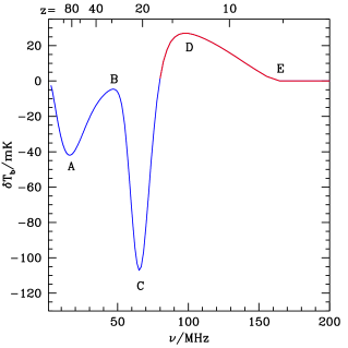
Figure 3: Details of the 21-cm global signal as a function of frequency, relative to the CMB, for our fiducial signal model. The solid line shows the 21 cm global signal as it transitions from absorption (blue) to emission (red). The different turning points are labelled (see text for details).

The effect of varying the efficiency with which Ly$\alpha$ and X-rays are produced and find their way into the IGM was studied by Pritchard & Loeb (2010). The same paper proposed a useful parametrization of the time-evolution of the global 21-cm signal, which we adopt here. The signal is described by five turning points where the frequency derivative of the signal is equal to zero (so each corresponds to a local extremum of the signal). We label the turning points A–E (see Figure 3), in order from the highest to the lowest redshift, and the physical interpretation of each is as follows:

A

– a minimum during the dark ages where collisional coupling of the 21-cm spin temperature to the gas kinetic temperature begins to become ineffective;

B

– a maximum at the transition from the dark ages to the regime where Ly$\alpha$ pumping by UV from the first stars begins to become effective;

C

– a minimum as X-ray heating (caused by the first accreting black holes) starts to become effective, raising the mean temperature;

D

– a maximum where the heating has saturated, before the signal begins to decrease because of cosmic expansion and reionization, i.e. the beginning of the EoR;

E

– the endpoint of reionization, after which the signal is (very close to) zero.

In this paper, the six parameters corresponding to the frequency and $\delta T_{\mathrm{B}}$ of turning points B, C and D are varied, while the the positions of A and E are fixed at $(16.1\ \mathrm{MHz},-42\ \mathrm{mK})$ and $(180\ \mathrm{MHz},0\ \mathrm{mK})$ respectively. In the absence of exotic processes, turning point A depends only upon fundamental cosmological parameters and known physics and so its position is essentially known. Turning point E relates to the details of the reionization history and, while its position is highly unknown, here we focus on the first galaxies. The ability of global experiments to constrain reionization has been considered in some detail by Pritchard & Loeb (2010) and Morandi & Barkana (2011).

The 21-cm signal is modelled as a cubic spline interpolating these points and having zero derivative at the position of the turning points. We will consider constraints on these parameters to be the primary result of an experiment to measure the global 21-cm signal at these redshifts. Clearly, many other parametrizations are reasonable; for example, we could attempt to constrain directly the input parameters of a physical model for the global signal, such as the spectral shape of early stars or the fraction of Ly$\alpha$ which escapes early galaxies. We have chosen the ‘turning point’ parametrization because it is not as model-dependent, and because the 21-cm signal for a given set of parameters is very quick to compute, which is desirable for our Monte Carlo analysis. Turning points B, C and D, at around 45 MHz, 65 MHz and 100 MHz respectively, are visible in the spectrum shown in Fig. 8, and are shown in the context of a larger frequency range encompassing turning points A and E in Fig. 3.

3.2 Diffuse foregrounds

Perhaps the most important foreground for a global 21-cm experiment, in that it dominates in intensity and is present at some level for all pointing directions, is the diffuse emission coming from our Galaxy and external galaxies. Though the extragalactic foreground may be considered to come from discrete sources, we treat it as part of the diffuse foreground since the solid angle of the beam of our proposed experiment is so large (around 1–2 sr) that it averages together a great number of sources in any one pointing. The Galactic contribution is larger than the extragalactic contribution, and consists largely of synchrotron radiation, with a small contribution from free-free (e.g. Shaver et al., 1999).

Our model for the spatial variation of the diffuse foregrounds is the global sky model (GSM) of de Oliveira-Costa et al. (2008). The foreground temperature measured when the spacecraft is pointing in a given direction is obtained by convolving the GSM with the instrumental beam. We assume that we can observe eight approximately independent sky areas (since our simulated beam covers around one eighth of the sky, depending on frequency), and that this is done by pointing in eight different directions for equal amounts of time, with each direction being a vertex of a spherical cube. This gives us eight foreground spectra. These are modelled using a similar functional form to that used by Pritchard & Loeb (2010), i.e.:

$$\begin{split}\log T^{i}_{\mathrm{FG}}&=\log T^{i}_{0}+a^{i}_{1}\log(\nu/\nu_{0})+a^{i}_{2}[\log(\nu/\nu_{0})]^{2}\\ &\quad+a^{i}_{3}[\log(\nu/\nu_{0})]^{3}\ ,\end{split}$$ (2)

with $\nu_{0}=80\ \mathrm{MHz}$ being an arbitrary reference frequency which we choose to lie in the middle of our band, and $i=1,\ldots,8$ labels the different sky areas. The parameters $\{T^{i}_{0},a^{i}_{1},a^{i}_{2},a^{i}_{3}\}$ for $i=1,\ldots,8$ constitute the 32 parameters of our diffuse foreground model. The ‘true’ or input parameters are obtained from fits to the GSM spectrum for each region.

This approach somewhat simplifies the problem since we have ignored covariance between the different observed patches, treating them as independent. Instead, a realistic experiment would likely return a sky map containing a larger number of correlated pixels with approximately the same amount of information as our eight independent pixels. We leave a detailed study of map making and the handling of correlated pixels to future work. However, it seems likely that the overall effect of dealing properly with small correlations between the patches would be to increase the error bars on the final constraints slightly, since the foreground subtraction algorithm would have less information to work with. In an extreme case with a single all-sky integrated spectrum, the degeneracies between foreground, signal and instrument parameters would clearly be severe. This contrasts with the case for interferometric experiments, when knowledge of the correlation properties of the foregrounds may help somewhat with foreground subtraction since they have strong spatial correlations on scales larger than the pixel size in an interferometric map (Liu & Tegmark, 2011a). Correlations between pixels then work mainly to increase the effective signal to noise ratio of the measurement of the foreground in clusters of correlated pixels.

By restricting ourselves to a third order polynomial in $\log\nu$ in each pixel, we are focusing on a relatively optimistic case. Pritchard & Loeb (2010) showed that this was the minimal number of parameters needed to characterize the foreground model of de Oliveira-Costa et al. (2008), but the situation could be worse since this model is based on quite limited observational data; Petrovic & Oh (2011) have, however, given theoretical reasons to expect that the Galactic foregrounds should be very smooth. Moreover, a recent study by Liu & Tegmark (2011b) found that four effective parameters was sufficient to fit a foreground model with various components, with a total number of physical parameters several times larger. The studies of Pritchard & Loeb (2010) showed that increasing the order of the polynomial required to fit the foregrounds significantly worsened the constraining power of global 21 cm experiments. It would be straightforward to similarly explore the effects of foregrounds with more structure here, but rather than retrace old work we chose to focus on the effect of other sources of uncertainty.

3.3 Other foregrounds

3.3.1 The Sun

We find that it is important to include the quiet Sun in our modelling, since this significantly affects our constraints on the 21-cm history. Although the Sun is a bright radio source, it is compact rather than diffuse, so even if it lies at the centre of the antenna beam its power is diluted by a factor of the solid angle subtended by the Sun divided by the effective solid angle of the antenna beam. Fig. 2 shows its effective brightness temperature (the brightness temperature of an object with the same flux density but filling the beam) for this case. If the Sun lies away from the centre of the beam, its power is suppressed even more.

For some of the observing time of a lunar-orbiting antenna, the Sun will be entirely occluded by the Moon. For the rest of the time, the Sun’s position in the antenna beam will vary and it will contribute different amounts of power at different times, even if its intrinsic luminosity remains perfectly steady. For that reason, in our modelling, we assume that while the shape of the Sun’s spectrum remains the same, the overall contribution of the Sun (i.e. the normalization of its integrated spectrum) will be different in each of the eight sky areas we observe. Otherwise, our model for the Sun’s spectrum is similar to our model for the diffuse foreground spectrum, i.e.

$$\begin{split}\log T^{i}_{\mathrm{Sun}}&=\log T^{i,\mathrm{Sun}}_{0}+a^{\mathrm{Sun}}_{1}\log(\nu/\nu_{0})\\ &\quad+a^{\mathrm{Sun}}_{2}[\log(\nu/\nu_{0})]^{2}+a^{\mathrm{Sun}}_{3}[\log(\nu/\nu_{0})]^{3}\ ,\end{split}$$ (3)

where $i=1,\ldots,8$ again labels the different sky areas, but $a_{1}$, $a_{2}$ and $a_{3}$ do not carry an index, so that there are a total of 11 parameters to be fit. The input values of these parameters are derived from a fit to the solar spectrum shown by Zarka (2004), which yields $a_{1}=1.9889$, $a_{2}=-0.3529$ and $a_{3}=0.0407$. To our knowledge, there are no observations which probe the variability of the solar spectrum at the level of sensitivity required for our experiment, so it is possible that in reality it has small variations in time, and perhaps microbursts, contrary to our assumption. This may be tested in the next few years with ground-based observatories such as the Murchison Widefield Array (MWA) and the Long Wavelength Array. A full 3000 h dataset from our reference mission would allow the effect of the Sun on the final constraints to be tested by using only those observing times for which the Sun was occluded by the Moon.

Because we know the position of the Sun in the beam at all times during our observations, and because ground-based observations of the Sun with smaller beams than our proposed antenna may provide good independent constraints on the solar spectrum, it is possible that quite good priors may be placed on the parameters in Equation (3). In Section 5 we consider cases where these parameters are treated as being completely free and fit only by the satellite data, and cases where good priors are placed on them beforehand. The different shapes of the spectra of the diffuse foregrounds and the Sun may lead one to worry that combinations of the parameters of these sources may be degenerate with the parameters of the 21-cm signal. In this case, what will help to disentangle the 21-cm signal from the foregrounds is that the former is identical between different sky areas (because the antenna beam averages over such an enormous volume of the high-redshift Universe) while the latter varies spatially. It may also be possible to arrange that one or two sky areas may be observed only when the Sun is occluded by the Moon. Except where stated otherwise, our results below assume that two out of the eight sky areas have always been observed when this is the case. Were this not true, one may still be able to check that results obtained excluding times during which the Sun is in view are consistent with results from the full data set. This assumption does not make a significant difference to our results, but it does allow us to examine how the presence or absence of the Sun in a given sky area changes the correlation properties of the parameters in Section 5.1.

During a solar burst, the radio power of the Sun can increase by several orders of magnitude, and we would not anticipate using data gathered during a solar burst for 21-cm work. The strength of the bursts means, however, that they can be identified quite straightforwardly, and data gathered during a burst can be excluded unless the Sun is occluded by the Moon at the time. The excluded periods would be short compared to the lifetime of the mission (between a few seconds and $\sim\!1$ hr; Wild, Smerd & Weiss, 1963), and there are approximately tens of such bursts per year, depending on the phase in the solar cycle (Gopalswamy et al., 2008). Therefore we do not expect them to significantly affect the sensitivity of the experiment.

3.3.2 The Moon

The Moon itself is a thermal radio source, with different radio wavelengths probing its temperature at different depths. In our band, the temperature is $\approx 220\ \mathrm{K}$ (e.g. Salisbury & Fernald, 1971; Keihm & Langseth, 1975). Since the antenna will always be pointing towards the sky rather than towards the lunar surface, the Moon’s contribution will be suppressed, though some radiation will enter through the antenna’s back- and sidelobes. Thus, its mean effective contribution, shown in Fig. 2, ends up being around 20 K. We model the Moon’s radiation using a single parameter – its temperature – and neglect any frequency dependence, or dependence on phase in the lunar cycle, which is expected to be weak given the depth probed by these long wavelengths. Clearly this may be an oversimplification, but the data we have found do not yet seem precise enough to suggest any specific, more sophisticated model, so this is an area that may require further study. If the emission from the Moon is more complicated, it is possible that the modulation of its signal as it enters more or less sensitive areas of the beam may help disentangle it from the other sources, or that pointing the antenna towards the Moon for some time may help constrain its emission at the expense of a small amount of data collection time. An analysis would then require the use of the full time series of spectra from the satellite, rather than just the eight integrated spectra we look at here, and is therefore beyond the scope of the current paper.

The Moon also reflects some of the radiation from the Galaxy and other sources, and has a reflectivity of around 5–10 per cent (e.g. Davis & Rohlfs, 1964). We assume that this is constant with frequency, so that the fraction of the incoming radiation which is reflected is a single parameter in our model. The input value for this parameter is chosen to be 10 per cent, though the true value is uncertain. This reflected radiation is further suppressed, by a factor of around 10, since it enters through the backlobe of the antenna, so that the effective temperature of the reflected foregrounds, shown in Fig. 2, is around two orders of magnitude below that entering the antenna directly from the front.

3.3.3 Neglected contributions

There are some other processes which one would expect to contribute to the spectra but which are not explicitly included in the modelling. We describe some of them here, and justify neglecting them in this analysis.

Firstly, other planets, especially Jupiter, are known to be radio sources at these frequencies. We expect Jupiter to have a qualitatively similar effect on our results as the Sun, but taking into account the small solid angle Jupiter subtends compared to the size of our antenna beam it is fainter than the Sun by a factor of around $10^{-4}$ (using data from Zarka, 2004), and so we neglect it here. Jupiter does experience intense bursts, but their spectrum cuts off very sharply above around 40 MHz, so they are not expected to intrude into our band.

Radio recombination lines (RRLs; Peters et al., 2011) may comprise a foreground which is not spectrally smooth. They are caused by transitions of electrons between atomic energy levels with very large principal quantum numbers, and can be seen either in absorption or emission depending on frequency. So far, the only RRLs detected have been from carbon atoms in our own Galaxy. The lines are narrow (around 10 kHz) and occur at known frequencies. The high resolution of our unbinned spectra would therefore allow them to be detected (if present) and removed while only discarding a very small fraction of the data and having a negligible effect on our sensitivity. Indeed, this is the main reason for requiring high spectral resolution. Since we deal only with binned spectra in this paper, the RRLs are assumed to have been excised before the rest of the analysis takes place, and we do not include the effect of these excisions on the noise levels of the binned spectra. It is possible that the integrated contribution of RRLs from external galaxies (redshifted by various amounts) would leave smoother low-level features in the spectrum. This contribution has been estimated by Petrovic & Oh (2011) to be very small, however. Moreover, it is unclear whether it could mimic the spectral features expected in the 21-cm signal and, unlike the signal, it would not be constant over the sky.

The relatively low altitude of the assumed lunar orbit means that the spacecraft will encounter dust particles from the highly tenuous upper layers of the lunar exosphere. Dust impacts at orbital speeds produce puffs of plasma which generate an electrical response in the antenna (Meyer-Vernet, 1985), and therefore could be a source of noise. A calculation of the noise power using a model for the height distribution of lunar dust (Stubbs et al., 2010) and for the surface area of the spacecraft, however, gives the noise spectrum shown in Fig. 2, at least an order of magnitude below the thermal noise in a very deep integration, and so we neglect dust impacts in this work.

Finally, we ignore noise or RFI reflections from other spacecraft which may be visible from a low altitude orbit over the lunar far side, such as others which orbit the Moon, or those positioned at the Earth-Moon $\mathrm{L}_{2}$ point. Reflections of RFI from the sunshade of the James Webb Space Telescope, for example, would be around $10^{-7}$ of the thermal noise.

3.4 The instrument

Our model for instrumental effects on the measured spectrum caused by the radiometer system (antenna, amplifiers, receiver and digital spectrometer) is based on that used for EDGES (see Bowman & Rogers, 2010, in particular the supplementary information). Internal calibration is performed by switching the input between the antenna and calibration loads. While a very precise absolute calibration is not necessary, it is important that the relative calibration of different channels is very accurate, since spectral smoothness at a level of one part in $10^{6}$ is used during foreground removal, and a relative calibration error could be confused with variations in the sky spectrum. For wide-band systems such as DARE or EDGES, the canonical internal calibration equation for a radiometer (e.g. Bowman et al., 2008, their eqn. 3) is insufficient because the impedance of the antenna varies strongly with frequency and is not well-matched to the impedance of the receiver front-end amplifier across the entire band as it would be for a narrow-band system. The primary result is that noise power emitted from the amplifier toward the antenna (which is usually neglected in narrow-band systems) can be reflected back into the receiver. This noise can be correlated with the downstream receiver noise producing constructive and destructive interference as a function of frequency in the measured spectrum with a period related to the electrical path length between the receiver and the antenna. In order to account for this uncalibrated spectral component, we use the noise wave propagation model (Penfield, 1962; Meys, 1978; Weinreb, 1982; Bowman & Rogers, 2010) to represent the interaction of a noisy receiver amplifier and the antenna impedance. Following Meys (1978, his eqns. 5 and 6), we have:

$$\begin{split}T_{\mathrm{ant}}(\nu)&=T_{\mathrm{a}}+|\Gamma(\nu)|^{2}T_{\mathrm{b}}+2T_{\mathrm{c}}|\Gamma(\nu)|\cos\left[\beta(\nu)+\phi_{\mathrm{c}}\right]\\ &\quad+T_{\mathrm{sky}}(\nu)\left[1-|\Gamma(\nu)|^{2}\right]\ ,\end{split}$$ (4)

where $T_{\mathrm{a}}$ is the standard noise from the output port of the amplifier (usually called the receiver noise), $T_{\mathrm{b}}$ is the noise directed toward the antenna from the input port of the amplifier, and $T_{\mathrm{c}}$ is the amplitude of the correlated components of $T_{\mathrm{a}}$ and $T_{\mathrm{b}}$ such that $T_{\mathrm{c}}=\epsilon\sqrt{T_{\mathrm{a}}T_{\mathrm{b}}}$, where $\epsilon$ is the amplitude of the correlation coefficient and the parameter $\phi_{\mathrm{c}}$ in Eqn. (4) gives the phase of the correlation. $T_{\mathrm{sky}}$ is the total sky brightness ($T_{\mathrm{21\mbox{-}cm}}+T_{\mathrm{FG}}+T_{\mathrm{Sun}}+\ldots$) convolved with the antenna beam and $\Gamma(\nu)=|\Gamma(\nu)|\mathrm{e}^{i\beta(\nu)}$ is the reflection coefficient of the antenna due to this impedance mismatch with the receiver.

$T_{\mathrm{a}}$, $T_{\mathrm{b}}$, $T_{\mathrm{c}}$, $\phi_{\mathrm{c}}$, $\Gamma$ and $\epsilon$ can be computed for a theoretical model of the radiometer system, or estimated using measurements taken while the satellite is on the ground. It is possible, however, that they cannot be estimated to the required level of accuracy either way. Rather, they may have to be estimated using the science data themselves. In this paper, we assume that each of these parameters is constant as a function of frequency, with the exception of the complex reflection coefficient, $\Gamma$. We further restrict the receiver noise temperatures such that $T_{\mathrm{a}}\equiv T_{\mathrm{b}}$ always, and we neglect $\phi_{\mathrm{c}}$ since it can be absorbed into the $\beta$ term with no loss of generality. We set the input value of the receiver temperature to be 100 K and $\epsilon$ to be 0.1, retaining each as a single free parameter in our model. As was done for the antenna power pattern, $\Gamma(\nu)$ has been computed in an electromagnetic model of the DARE radiometer system (Burns et al., 2011). The computed $\Gamma(\nu)$ is shown in Fig. 4.

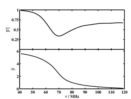
Figure 4: The reflection coefficient, $\Gamma(\nu)=|\Gamma|\mathrm{e}^{i\beta}$, due to the impedance mismatch between antenna and receiver for the simulated DARE radiometer system. The top panel shows $|\Gamma|$ and the bottom panel shows $\beta$ in radians. The sensitivity to the sky temperature scales as $1-|\Gamma|^{2}$.

From Eqn. (4), one can see that the sensitivity to the sky temperature scales as $1-|\Gamma|^{2}$, and so Fig. 4 demonstrates that the system is most sensitive at around 70 MHz, with the sensitivity tailing off somewhat at high frequency and significantly at low frequency. By design the frequency response is very smooth, to assist in foreground subtraction.

We also used this smoothness to guide us in finding a suitable parametrization for $\Gamma(\nu)$: we take as our parameters the ten lowest-frequency coefficients of the discrete cosine transform (DCT) of each of $|\Gamma(\nu)|$ and $\beta(\nu)$, giving us twenty parameters in total. The DCT was chosen as a simple and efficient way of modelling $\Gamma(\nu)$ as a sum of orthogonal functions. It was chosen after some experimentation with various transforms as the one which fit the simulated $\Gamma(\nu)$ to reasonable accuracy using a small number of coefficients. Since the DCT is also simply a special case of a real, discrete Fourier transform, it is very quick to compute. $\Gamma(\nu)$ depends on the properties of the various components of the antenna/receiver system, though, and so in future we may hope to find a more physically motivated parametrization that takes that into account. This would be useful if it could reduce the number of parameters in the model or the degeneracies between them. To find $\Gamma(\nu)$ given some set of parameters, we set all higher-frequency coefficients to zero and then compute the two inverse DCTs. Ten non-zero coefficients for each of $|\Gamma|$ and $\beta$ are used since this is the least number that allows us to fit the small ripples in the amplitude of the simulated reflection coefficient of our reference experiment at high frequency. The coefficients obtained thereby are the ones we use as the input to our modelling. When we refer to simulating a hypothetical ‘perfect’ instrument below, we take this to mean that $\Gamma(\nu)$ is known to be identically zero.

3.5 Thermal noise

The noise on the spectrum, for a spectral bin of width $B$ observed for a time $t$, is given by the radiometer equation:

$$\sigma(\nu)=\frac{T_{\mathrm{ant}}(\nu)}{\sqrt{2Bt}}\ ,$$ (5)

where the factor of $\sqrt{2}$ in the denominator arises from the two independent polarizations measured by a crossed dipole antenna. For an observation near the centre of our band, where the coldest areas of sky have $T_{\mathrm{sky}}\approx 1000\ \mathrm{K}$, and for $B=2\ \mathrm{MHz}$ and $t=375\ \mathrm{h}$ (corresponding to one of eight sky areas, observed for one eighth of the total integration time of 3000 h) this gives a noise of $0.4\ \mathrm{mK}$ in each spectral channel. This is roughly the level of noise above which Pritchard & Loeb (2010) found that constraints on the positions of turning points started to be seriously degraded in their Fisher matrix analysis. For such long integrations to be worthwhile, systematic sources of noise must also be controlled to at least this level; we assume that this is the case and do not attempt to model any additional systematic noise. Systematics one might worry about include, for example, temperature changes due to the spacecraft passing in and out of the shadow of the Moon as it orbits, which could affect the noise properties of the system, or leakage of noise from other components of the spacecraft itself. The design of the reference experiment is intended to minimize these effects: further details may be found in Burns et al. (2011).

4 Model fitting

For the fiducial case we consider, of a lunar-orbiting antenna measuring the spectrum of eight independent sky regions, our model for these eight spectra has 73 parameters:

• 6 for the 21-cm signal (frequency and temperature of three turning points);

• 32 for the diffuse foregrounds (coefficients of a third-order polynomial in each of eight sky regions);

• 11 for the Sun (a normalization parameter in each of eight different regions, plus three parameters describing the spectral shape);

• 2 describing the Moon (one for its temperature and one for its reflectivity);

• 22 describing the instrument (ten for the amplitude of the reflection coefficient, $|\Gamma(\nu)|$, ten for its phase, $\beta(\nu)$, and one each for $T_{\mathrm{rcv}}$ and $\epsilon$).

These parameters specify $T^{i}_{\mathrm{ant}}(\nu)$, where $i=1\ldots 8$ again runs over the different sky regions, and we can generate a simulated realization of the experimental data by adding noise to these spectra according to Eqn. (5). Having different sky regions in which the foregrounds are different but the 21-cm signal is the same helps to break the degeneracy between the foreground, signal and instrumental parameters. We use eight regions since averaging spectra into fewer sky regions would destroy information, while splitting the sky into more areas would mean the different spectra would not be independent, complicating the analysis.

Given the simulated noisy spectra, we find the best-fitting parameter values, and confidence regions on these values, using a Markov Chain Monte Carlo algorithm (MCMC; e.g.  Lewis & Bridle, 2002, and references therein) we have implemented in matlab. This provides an efficient way to explore a high-dimensional parameter space. Since there are many good references on MCMC, we only provide enough of a description of the technique here to establish some notation and allow us to be more precise about our particular implementation.

We seek to map the posterior probability distribution $P(\boldsymbol{\theta}|\boldsymbol{X})$ of the parameters of our model. $P$ is considered to be a function of the vector of parameters $\boldsymbol{\theta}$, with the vector $\boldsymbol{X}$, which contains our simulated data, held fixed. The posterior is related to the likelihood, $L(\boldsymbol{X}|\boldsymbol{\theta})$, by Bayes’ theorem,

$$P(\boldsymbol{\theta}|\boldsymbol{X})\propto L(\boldsymbol{X}|\boldsymbol{\theta})P(\boldsymbol{\theta}),$$ (6)

where $P(\boldsymbol{\theta})$ is the prior placed on the model parameters. For constant priors the likelihood gives us the posterior probability, up to an arbitrary multiplicative constant. Our goal is to see how well the parameters $\boldsymbol{\theta}$ may be inferred given an observed data set $\boldsymbol{X}$.

We assume that the noise in each frequency channel is Gaussian. Then, if $T^{i}_{\mathrm{ant}}(\nu_{j}|\boldsymbol{\theta})$ is the predicted antenna temperature in the $i^{\mathrm{th}}$ sky area in the $j^{\mathrm{th}}$ frequency channel given a parameter set $\boldsymbol{\theta}$, and $T^{i}_{\mathrm{meas}}(\nu_{j})$ is the ‘measured’ temperature in this sky area and channel in a simulated dataset, then the probability density of measuring this value is given by

$$p_{ij}=\frac{1}{\sqrt{2\pi\sigma_{i}^{2}(\nu_{j}|\boldsymbol{\theta})}}\mathrm{e}^{-[T^{i}_{\mathrm{meas}}(\nu_{j})-T^{i}_{\mathrm{ant}}(\nu_{j}|\boldsymbol{\theta})]^{2}/2\sigma_{i}^{2}(\nu_{j}|\boldsymbol{\theta})}$$ (7)

where $\sigma_{i}(\nu_{j}|\boldsymbol{\theta})$ is the rms noise in the channel, computed from $T^{i}_{\mathrm{ant}}(\nu_{j}|\boldsymbol{\theta})$, the bandwidth and the integration time using Eqn. (5). Then, assuming that each sky area and frequency channel is independent, the likelihood is given simply by

$$L(\boldsymbol{T}_{\mathrm{meas}}|\boldsymbol{\theta})=\prod_{i=1}^{\ n_{\mathrm{areas\phantom{q}}}}\prod_{j=1}^{n_{\mathrm{freq}}}p_{ij}\ ,$$ (8)

where $\boldsymbol{T}_{\mathrm{meas}}$ is a vector containing $T^{i}_{\mathrm{meas}}(\nu_{j})$ for all $i$ and $j$. Usually it is computationally simpler to work with $\log(L)$, for which the double product becomes a double sum.

We use the Metropolis-Hastings algorithm (Hastings, 1970) to generate a sequence of random samples from the posterior distribution; this sequence of samples is a chain. To see how the algorithm works, suppose the chain is at the position $\boldsymbol{\theta}_{n}$ in parameter space. We randomly generate another parameter vector, $\boldsymbol{\theta}_{n+1}$, according to the ‘proposal density’ $q(\boldsymbol{\theta}_{n},\boldsymbol{\theta}_{n+1})$. This vector is accepted as the next link in the chain with a probability

$$\alpha(\boldsymbol{\theta}_{n},\boldsymbol{\theta}_{n+1})=\min\left\{1,\frac{P(\boldsymbol{\theta}_{n+1}|\boldsymbol{X})}{P(\boldsymbol{\theta}_{n}|\boldsymbol{X})}\right\}\ ,$$ (9)

if $q$ is symmetric, which is true for the proposal densities we use. Over time the chain will explore the full parameter space with statistical properties that allow a set of unbiased and random samples to be extracted.

Clearly the position of successive samples is correlated. To reduce this correlation and obtain approximately independent samples, we ‘thin’ the chain, retaining only one out of every $n_{\mathrm{thin}}$ samples. The results we show here use $n_{\mathrm{thin}}=50$, which allows us to run the chains long enough to reach convergence without having to store an extremely large number of samples. The first $n_{\mathrm{burn\mbox{-}in}}$ thinned samples are discarded to ensure we only use samples from the equilibrium distribution; we find $n_{\mathrm{burn\mbox{-}in}}=10^{4}$ to be sufficient.

The choice of the proposal density, $q$, strongly affects the computational efficiency of the algorithm. A $q$ which is too broad makes the acceptance ratio, $\langle\alpha\rangle$, very small, meaning we have to draw from $q$ and compute $L$ many times to obtain each new link in the chain. A $q$ which is too narrow forces us to take only tiny steps in parameter space, preventing us from mapping its interesting regions in a reasonable amount of time. To avoid either of these scenarios, we automate the choice of $q$. This requires us first to estimate the parameter covariance matrix, C. For the first $2n_{\mathrm{burn\mbox{-}in}}$ thinned samples following burn-in, we compute an estimate of C from an estimate of the Hessian of the posterior, using the derivest package. For subsequent samples, we instead estimate C directly from the cloud of existing samples, which we have found to be more robust. The covariance matrix, being costly to compute, is recalculated only after every $10^{5}$ evaluations of the posterior. Because the proposal distribution changes during a run, this means that the chains are no longer strictly Markov. During the preparation of this manuscript, however, it came to our attention that this approach is very similar to the ‘Adaptive Metropolis’ algorithm of Haario, Saksman & Tamminen (2001), who prove that the chain none the less has the desired ergodicity properties and converges correctly to the equilibrium solution.

Having found C, we proceed to find a basis of parameter space in which it is diagonal, and denote by $\tilde{\boldsymbol{\theta}}$ the vector of parameters in this new basis. We choose a random subset of these parameters, $\{\tilde{\theta}_{i_{1}},\tilde{\theta}_{i_{2}},\ldots,\tilde{\theta}_{i_{n_{\mathrm{vary}}}}\}$ to vary at each step, where $n_{\mathrm{vary}}$ is a numerical parameter we may choose. Taking $n_{\mathrm{vary}}=1$ typically gives us acceptance ratios of around 70 per cent. The proposal distribution $q$ for this subset of the (transformed) parameters is then taken to be a multivariate Gaussian distribution, with a diagonal covariance matrix equal to that of the full parameter set, but keeping only the rows and columns numbered $i_{1},i_{2},\ldots,i_{n_{\mathrm{vary}}}$. This choice appears to perform well in practice.

We obtain around $10^{5}$ thinned samples in a few hours on a 2.3 GHz AMD Opteron processor. By running eight different chains we can apply the convergence test of Gelman & Rubin (1992), which confirms the impression from a single chain that using this many samples is sufficient for good convergence.

An example of marginalized parameter distributions obtained using this method for a particular noise realization is shown in Fig. 5. In this case we assume a perfect instrument ($\Gamma(\nu)\equiv 0$) observing eight sky areas for a total of 3000 h, i.e. 375 h per sky area. Each panel shows the joint distribution of the frequency and temperature of one of the turning points of the 21-cm signal. We also show the position of the input value of the parameters and the parameter values with the highest posterior probability. The difference between these gives a sense of how robustly the parameters may be recovered or whether the recovered parameters may be biased in some way by the foreground removal process. We will use this format for displaying most of our results.

For this particular noise realization, the input parameter values for two turning points lie within the 68 per cent confidence region, while those for the third lie just outside its border, suggesting that the parameters have been recovered without significant bias, even for the most difficult turning point at low frequency (turning point B). Further, the size of the confidence regions is small and, thus, very promising, allowing the three turning points to be distinguished clearly from one another.

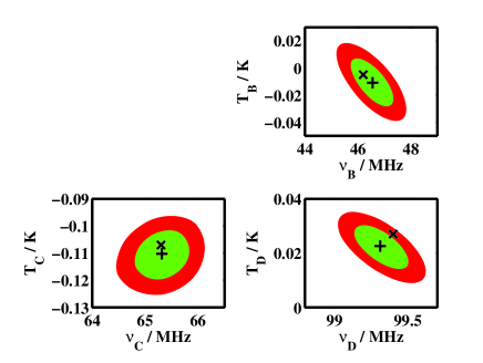
Figure 5: Confidence regions on turning points B, C and D of the cosmological signal, assuming a perfect instrument observing eight areas of the sky for a total of 3000 h. The 68 per cent confidence region is in green, and the 95 per cent confidence region is in red. For each turning point, the frequency of the turning point is on the $x$ axis and the brightness temperature on the $y$ axis. The ‘+’ shows the best-fitting parameter values, while the ‘$\times$’ shows the parameter values which were used as inputs to the simulation.

5 Results and discussion

Having looked at signal recovery for a perfect instrument, we now move on to a more realistic case based on the simulated properties of the proposed DARE satellite. We start by assuming that there is no meaningful prior information on any of the parameters, so that they are constrained only by the satellite science data. The confidence regions for this case, for a single random noise realization assuming a total of 3000 h of integration time (375 h per sky area), are shown in Fig. 6. It is easy to see, noting the difference in axis scale between Figs. 5 and 6, that the parameter constraints are significantly degraded. The frequency of turning point C, for example, is found with an error of around $\pm 1\ \mathrm{MHz}$, rather than $\pm 0.5\ \mathrm{MHz}$ from a perfect instrument. The best-fitting values of all the parameters are somewhat offset from the true values, but the error appears to be consistent with the confidence regions estimated from MCMC. Turning point B is worst affected: the 68 per cent confidence region spans a range of well over 100 mK in temperature, and extends in frequency to below the bottom end of the range (40 MHz), where we have truncated the scale of the plot. The constraint on its frequency is therefore very model-dependent, and is probably best viewed as an upper limit, ruling out a turning point above $\sim 48\ \mathrm{MHz}$ with 95 per cent confidence (this upper limit is properly computed from the fully marginalized, one-dimensional probability distribution of $\nu_{\mathrm{B}}$; see Table 1).

The temperature of the other turning points is not as well determined as their frequency, in the sense of how constraining the limits would be for models of the dark ages, but some measurements are still obtained. For all three turning points, the temperature is slightly underestimated. This is simply because the temperature errors are correlated across the band rather than because of some bias in the method: we examine the correlations further in Section 5.1. The correlation arises because of the difficulty of measuring the overall normalization of the signal (as opposed to its spectral variation) in the presence of the strong foregrounds.

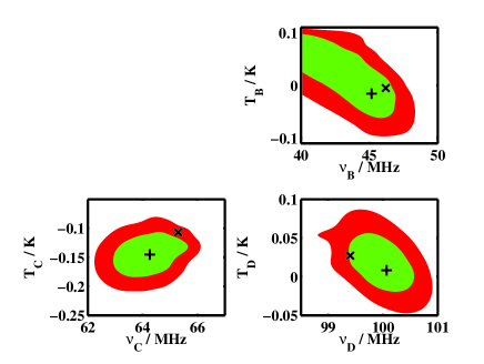
Figure 6: Confidence regions on turning points B, C and D of the cosmological signal, assuming a realistic instrument, and that we have no prior information on the parameters of the instrument model and the solar spectrum. Eight sky regions are observed for a total of 3000 h. Colours and symbols are as for Fig. 5, but for this and all subsequent figures the axis scales vary.

Even though the parameter constraints may look weak compared to the case for the perfect instrument of Fig. 5, the foreground parameters are very well constrained. For example, the spectral index in one of the sky regions at $80\ \mathrm{MHz}$ is found to be $-2.350898\pm 0.000042$ (2-$\sigma$ errors), compared to a true value of $-2.350903$. This illustrates the dynamic range required for such an experiment. The Sun, being a weaker source, does not have its spectral index determined quite so well: we find a value of $1.991\pm 0.011$ at $80\ \mathrm{MHz}$, with the true value being $1.989$.

Fig. 7 shows how the constraints are improved if we impose tight, Gaussian priors on the parameters of the non-diffuse foregrounds and the instrument, again assuming 3000 h of observation. $T_{0}^{i,\mathrm{Sun}}$ is assumed to be known to 0.1 per cent for all $i$, as are the temperature and reflectivity of the Moon, while $\{a_{1}^{\mathrm{Sun}},a_{2}^{\mathrm{Sun}},a_{3}^{\mathrm{Sun}}\}$ are known with an error of $\pm 0.001$. The coefficients of $\Gamma(\nu)$ are known to one part in $10^{6}$ (i.e. almost perfectly), while $T_{\mathrm{rcv}}$ and $\epsilon$ are known to 0.1 per cent. The assumption that the reflection coefficient is known to one part in $10^{6}$ is well beyond typical expectations at present, and is thus an optimistic prior. Most antennas are characterized at the 1 per cent level today, but devices designed to make accurate impedance measurements are stated in their specifications to perform to an accuracy of $<0.1$ per cent, and it is reasonable that this level could be achieved. This topic is being actively worked on with EDGES, the closest current analogue to DARE, in the field and the laboratory, with a target of achieving an accuracy of one part in $10^{4}$. Furthermore, it should be possible to treat the unknown aspects of the reflection coefficient with more physically motivated models than the DCT, which would help to reduce the effective degrees of freedom and so approach the desired accuracy. Our priors on $T_{\mathrm{rcv}}$ and $\epsilon$ are more plausible, and they could well be measured in the lab to this level before launch.

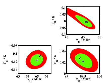
Figure 7: Confidence regions on turning points B, C and D of the cosmological signal, assuming a realistic instrument observing eight sky regions for a total of 3000 h, but with tight priors on the parameters of the instrument model, the solar spectrum and the properties of the Moon. We assume here, as throughout, that there is no prior information on the parameters of the diffuse foregrounds or the 21-cm signal itself. Colours and symbols are as for Fig. 5.

Under these conditions, the parameter constraints approach more closely those for the perfect instrument of Fig. 5. The main exception is that it becomes harder to rule out turning point B lying at a much lower frequency and higher temperature. A good measurement can only be found at 68 per cent confidence. The 95 per cent confidence region extends outside the band for which we have data, and any inferences about the properties of the signal in that region depend strongly on the assumed signal model. The shape of the confidence region suggests that our data actually tell us the amplitude and slope of the signal at low frequency, and that turning point B lies somewhere on a curve consistent with that amplitude and slope within the errors.

Since the instrumental frequency response and the non-diffuse foregrounds are well known, the weak constraint on turning point B compared to the perfect instrument must occur because of the reduced sensitivity at low frequencies, caused by the large value of $|\Gamma(\nu)|$ there. To find the position of turning point B precisely, it may be necessary to have an instrument with better sensitivity at low frequency, and possibly a lower minimum frequency. This is difficult to achieve (see the steep drop in sensitivity at low frequencies in Fig. 4), though one possible route would be a larger antenna and ground screen, which may be awkward and expensive for a satellite mission. Even then, it is hard to design an antenna which can cover a frequency range which is more than a factor of $\sim\!3$ without (for example) the antenna changing mode at the top end of the frequency range and introducing frequency structure into the response. The large uncertainty in current theoretical models of the signal means that an instrument with a range of, say, $35$–$105\ \mathrm{MHz}$ would run the risk of missing out entirely on turning point D, which we would otherwise hope to constrain quite precisely. Figure 7 suggests we are close enough to a measurement of turning point B that this may be possible with some smaller tweak to the design without having to change the current DARE frequency range.

We show how the parameter constraints of Fig. 7 translate into constraints on the shape of the 21-cm signal in Fig. 8. Here we plot the true signal, the mean over all the samples of the extracted signal at each frequency, and a 68 per cent confidence interval around this mean. The shape of the signal is recovered quite well, but the frequency of the turning points seems, visually, to be recovered more accurately than the temperature. The absolute normalization of the curve is difficult to determine.

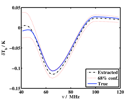
Figure 8: The mean extracted signal (dot-dashed black line) and 68 per cent confidence limits on this mean (dashed red lines) are compared to the ‘true’ signal constructed from the input parameters to the simulation (solid blue line). This plot assumes an instrument observing eight areas of the sky for a total of 3000 h, with tight priors on the parameters concerning the instrument, the Sun and the Moon, as in Fig. 7.

The width of the error bars is larger at the lower end of the frequency range than at the upper end, but not to the extent that would be expected if one were simply to use the rms thermal noise at each frequency to determine the error bar, since the sky temperature in the lowest frequency channel is $>10$ times that in the highest frequency channel, and this is the most important contributor to the thermal noise. Instead, the errors across the whole band are highly correlated, since the shape of the signal is reconstructed only from the six parameters giving the position of the turning points.

Before moving on from the case where we have good prior information on the properties Sun, Moon and instrument, we illustrate the errors on individual parameters which can be achieved in this case by showing the marginalized distributions of a subset of them in Fig. 9. It is also reassuring to be able to check that the distributions seem fairly smooth and well behaved. Complicated, multimodal distributions (or, for example, strongly curving degeneracies between different parameters) would be awkward for the sampler we have implemented here, and might require a more sophisticated method to sample them efficiently.

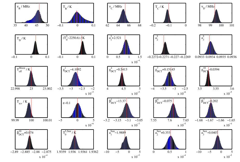
Figure 9: 1D marginalized distributions of the parameters for the case when we have tight priors on the properties of the instrument, the Sun and the Moon, as in Figs. 7 and 8. The vertical, red, dashed line shows the input value of the parameter. The names of the parameters given in each panel are as in the text, except that the discrete cosine transform coefficients of $|\Gamma|$ and $\beta$ are labelled $g_{\mathrm{DCT}}^{i}$ and $\beta_{\mathrm{DCT}}^{i}$ respectively.

We now wish to consider whether the improvement between Fig. 6 and Fig. 7 comes from our better knowledge of the non-diffuse foregrounds (in particular the Sun) or of the instrument. To this end, in Fig. 10 we show results obtained using the tight priors on $\Gamma(\nu)$ given above, but reverting to weak priors on the spectral parameters of the Sun.

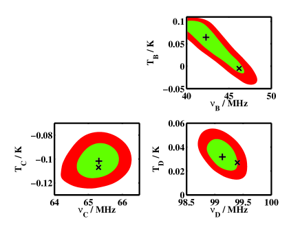
Figure 10: Confidence regions on turning points B, C and D of the cosmological signal, assuming a realistic instrument observing eight sky regions for a total of 3000 h, but with tight priors on the parameters of the instrument model. Colours and symbols are as for Fig. 5.

The results for turning points C and D are almost as good as for the previous case, showing that superb knowledge of the instrument is the most important factor in extracting the 21-cm signal accurately, though constraints on turning point B are noticeably degraded. Foreground parameters are also measured more precisely than for the case of Fig. 6: for example, the error on the spectral index of the Sun at 80 MHz is reduced by a factor of about six. If the instrumental calibration can be improved by using the spectra at full time and frequency resolution, or by introducing extra mechanisms for internal calibration, then this would clearly be very desirable, and should be the subject of further study.

By contrast with Fig. 10, Fig. 11 shows the confidence regions we derive when we assume tight priors on the spectrum of the Sun (obtained perhaps by ground-based observations), but relax the priors on the coefficients of the instrumental response to their original size. The constraints on the signal parameters are improved only a little over those of Fig. 6, with the overall temperature normalization being especially hard to recover. None the less, external constraints on the solar spectrum would be valuable as a consistency check.

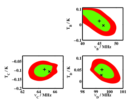
Figure 11: Confidence regions on turning points B, C and D of the cosmological signal, assuming a realistic instrument observing eight sky regions for a total of 3000 h, and with tight priors on the parameters of the solar spectrum and the Moon. Colours and symbols are as for Fig. 5.

Finally, we look at the effect of changing the available integration time. Results so far have used 3000 h of data; for Fig. 12 we assume instead only 1000 h of data, as may occur if the satellite is able to observe for only one year. Otherwise, the assumptions are the same as for Fig. 7, i.e. tight priors on both the instrument and the non-diffuse foregrounds are assumed.

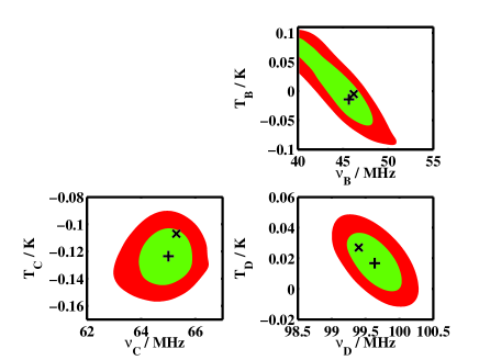
Figure 12: Confidence regions on turning points B, C and D of the cosmological signal, assuming a realistic instrument observing eight sky regions for a total of 1000 h, and with tight priors on the parameters of the instrument model, the solar spectrum and the Moon. Colours and symbols are as for Fig. 5. This figure should be compared to Fig. 7, which makes the same assumptions and differs only in the amount of integration time.

Table 1: 95 per cent confidence intervals (or, in some cases, upper and lower limits) on the frequency, redshift and temperature of turning points B, C and D for the various sets of assumptions we have considered. The first column gives a brief description of each simulation, while the second shows which figures were plotted using data from that simulation. The remaining columns show the constraints. The first row shows the true input values of the parameters, for comparison. All simulations assume 3000 h of observation, unless otherwise stated. A fuller description of each model is given in the relevant figure captions.

		Turning point B			Turning point C			Turning point D
Description	Figures	$\nu/\mathrm{MHz}$	$z$	$T/\mathrm{mK}$	$\nu/\mathrm{MHz}$	$z$	$T/\mathrm{mK}$	$\nu/\mathrm{MHz}$	$z$	$T/\mathrm{mK}$
True input values	-	46.2	29.7	$-5$	65.3	20.8	$-107$	99.4	13.29	27
Perfect instrument	5	$46.6^{+0.9}_{-1.1}$	$29.5^{+0.7}_{-0.6}$	$-10^{+22}_{-22}$	$65.3^{+0.7}_{-0.6}$	$20.7^{+0.3}_{-0.2}$	$-111^{+11}_{-11}$	$99.3^{+0.3}_{-0.2}$	$13.30^{+0.03}_{-0.03}$	$23^{+9}_{-12}$
No prior information	6,14	$<47.6$	$>28.8$	$55^{+45}_{-112}$	$64.3^{+1.3}_{-1.6}$	$21.1^{+0.6}_{-0.5}$	$-141^{+43}_{-55}$	$100.0^{+0.7}_{-0.8}$	$13.21^{+0.11}_{-0.10}$	$8^{+61}_{-41}$
All tight priors	7,8,9	$45.6^{+2.4}_{-5.2}$	$30.1^{+4.1}_{-1.5}$	$-7^{+84}_{-42}$	$65.0^{+0.8}_{-0.9}$	$20.9^{+0.3}_{-0.3}$	$-116^{+18}_{-17}$	$99.5^{+0.4}_{-0.3}$	$13.27^{+0.05}_{-0.05}$	$23^{+17}_{-15}$
Tight inst. priors	10	$42.6^{+4.8}_{-3.1}$	$32.3^{+2.7}_{-2.3}$	$95^{+6}_{-111}$	$65.3^{+0.7}_{-0.8}$	$20.7^{+0.3}_{-0.2}$	$-102^{+18}_{-17}$	$99.1^{+0.4}_{-0.3}$	$13.33^{+0.05}_{-0.05}$	$32^{+18}_{-14}$
Tight non-inst. priors	11	$<49.0$	$>28.0$	$25^{+75}_{-65}$	$64.7^{+1.3}_{-1.6}$	$21.0^{+0.5}_{-0.4}$	$-94^{+34}_{-52}$	$99.6^{+1.0}_{-0.8}$	$13.26^{+0.11}_{-0.13}$	$51^{+35}_{-48}$
1000 h integration	12	$<48.9$	$>28.1$	$-11^{+108}_{-51}$	$65.0^{+1.1}_{-1.5}$	$20.9^{+0.4}_{-0.4}$	$-125^{+26}_{-24}$	$99.6^{+0.5}_{-0.4}$	$13.26^{+0.07}_{-0.08}$	$17^{+24}_{-22}$
10000 h integration	13	$46.9^{+1.5}_{-4.4}$	$29.3^{+3.2}_{-1.0}$	$-9^{+71}_{-22}$	$65.4^{+0.7}_{-0.5}$	$20.7^{+0.2}_{-0.2}$	$-98^{+16}_{-11}$	$99.4^{+0.2}_{-0.3}$	$13.30^{+0.03}_{-0.03}$	$35^{+11}_{-11}$

The effect is as one might expect, with confidence regions on the parameters being enlarged somewhat. Turning points C and D can still be localized: a single year of data from our reference experiment could yield a detection of the first astrophysical sources of heating in the Universe, and the start of the epoch of reionization. It becomes impossible to obtain anything other than an upper limit on the frequency of turning point B, however: the sensitivity at the low frequencies is simply not sufficient for a clear measurement of its position.

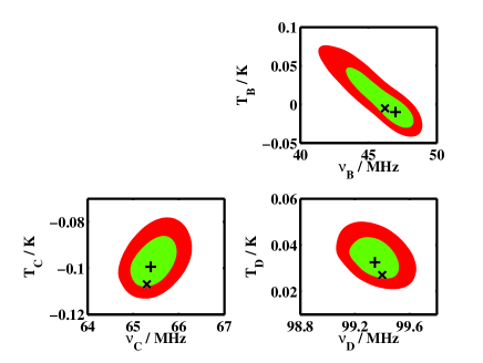
Figure 13: Confidence regions on turning points B, C and D of the cosmological signal, assuming a realistic instrument observing eight sky regions for a total of 10000 h, and with tight priors on the parameters of the instrument model, the solar spectrum and the Moon. Colours and symbols are as for Fig. 5. This figure should be compared to Figs. 7 and 12, which make the same assumptions and differ only in the amount of integration time.

To make sure that a realistic instrument can find a firm, 2-$\sigma$ detection of the frequency of turning point B given sufficient integration time, we show results for 10000 h of observation in Fig. 13. In this case the 2-$\sigma$ contours do indeed close above $40\ \mathrm{MHz}$, though there is still a significant degeneracy between the frequency and temperature of turning point B. The positions of turning points C and D are measured with improved accuracy compared to our baseline case, though further study of such deep integrations may need the possible systematics to be considered more carefully. An integration of this length would be challenging from space, needing either a mission of long duration or a very high observing efficiency (possibly both). It is likely that the requisite noise level in the vicinity of turning point B can be achieved more easily by modifications to the design of the spacecraft or radiometer system. Better constraints on turning point B might also come by extending the frequency coverage to lower frequencies.

We summarize the constraints on the parameters of the signal for all the different assumptions we have considered in Table 1. Here, we show 95 per cent confidence intervals (or, in some cases, upper or lower limits) on the frequency, redshift and temperature of the turning points, and record the figures for which each set of assumptions was used.

5.1 Correlation between parameters

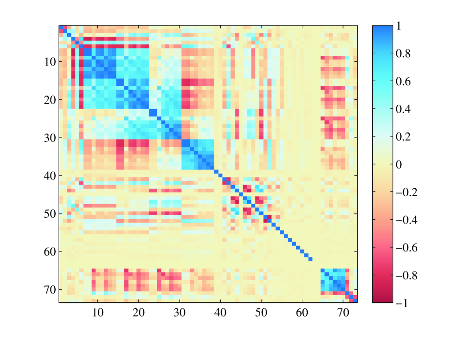
Figure 14: The scaled covariance matrix of all the parameters of the model, for a realistic instrument and assuming no meaningful prior information on the parameter values, as for Fig. 6. By the ‘scaled’ covariance matrix, we mean the that each pixel shows the correlation coefficient between two parameters, where a value of zero implies no correlation, and a value of 1 ($-1$) means perfect (anti-)correlation. The 1s on the diagonal come about because each variable is perfectly correlated with itself. The order of the parameters is given in Table 2. Note that parameters 63 ($T_{0}^{1,\mathrm{Sun}}$) and 64 ($T_{0}^{2,\mathrm{Sun}}$) are set to be identically zero since the Sun is assumed to be occluded by the Moon in sky regions 1 and 2, which accounts for the obvious stripe at this position. This figure is best viewed in colour, to make the difference between correlations (blue) and anticorrelations (red) more clear.

Table 2: Numbering of the rows of the scaled covariance matrix in Fig. 14

Row/column number	Parameter description
1–2	Frequency and temperature of turning point B
3–4	Frequency and temperature of turning point C
5–6	Frequency and temperature of turning point D
7–14	$T_{0}^{i}$, i=1,…,8
15–22	$a_{1}^{i}$, i=1,…,8
23–30	$a_{2}^{i}$, i=1,…,8
31–38	$a_{3}^{i}$, i=1,…,8
39	Effective temperature of the Moon
40	Reflectivity of the Moon
41–50	Discrete cosine transform coefficients of $|\Gamma(\nu)|$
51–52	$T_{\mathrm{rcv}}$ and $\epsilon$
53–62	Discrete cosine transform coefficients of $\beta(\nu)$
63–70	$T_{0}^{i,\mathrm{Sun}}$, i=1,…,8
71–73	$a_{1}^{\mathrm{Sun}}$, $a_{2}^{\mathrm{Sun}}$ and $a_{3}^{\mathrm{Sun}}$

The contour plots we have shown allow one to see clearly if the inferred frequency and temperature of a given turning point are correlated, or in other words if there is a degeneracy between these two parameters. The frequency, $\nu_{\mathrm{B}}$, and temperature, $T_{\mathrm{B}}$, of turning point B, for example, are clearly anticorrelated in all our figures. Such correlations may exist between all our parameters, and allow one to pick out possible degeneracies. Therefore, in Fig. 14, we show a scaled version of the covariance matrix of the parameters, such that a value of 1 ($-1$) in pixel $\{i,j\}$ indicates that the value of parameters $i$ and $j$ in the MCMC samples is perfectly (anti-)correlated, with a value of zero indicating no correlation. The key to the numbering of the rows and columns of the image is given in Table 2.

As expected, parameters 1 and 2 ($\nu_{\mathrm{B}}$ and $T_{\mathrm{B}}$) are easily seen to be anticorrelated, with the correlation coefficient between them here being $-0.69$. Other strong correlations are clearly apparent. For example, the block structure near the diagonal comes about because the parameters within one group, such as the normalization of the foreground temperatures in the different regions, $T_{0}^{i}$, are strongly correlated with each other. When a parameter outside this group is varied, the foregrounds in each region will all have to change in a similar way to compensate, introducing a correlation.

Some of the other features of the covariance matrix are straightforward to understand. For example, the temperatures of turning points C and D are strongly anticorrelated with the foreground temperature, $T_{0}^{i}$, for all $i$: an overall increase in the brightness temperature of the 21-cm signal can be compensated for by a decrease in the brightness of the foregrounds in every region of the sky. This very strong anticorrelation may help to explain why the inferred temperatures of the turning points become positively correlated with each other, an effect which is evident in many of our figures. It is more difficult to find ‘interesting’ constraints on the temperatures of the turning points than on the frequencies. The similar temperature offsets of the different turning points for any given noise realization may, however, allow us to recover the overall shape of the signal well, even if its absolute normalization is uncertain. The anticorrelation between the temperature of turning point B and the foreground temperature is less strong than for the other turning points, but this is mainly because of the larger statistical error on the temperature of turning point B.

The difficulty of pinning down the overall normalization of the 21-cm signal might be mitigated somewhat if we could fix its temperature at some frequency using external or theoretical constraints. To some extent we do this already by fixing the positions of turning points A and E, which lie outside the observed band, and this appears to be insufficient. The best candidate for a normalizing point inside the DARE band is probably turning point D: looking at Equation (1), if $x_{\mathrm{HI}}\approx 1$ (reionization not yet seriously under way) and $T_{\mathrm{S}}\gg T_{\gamma}$ (heating has saturated), the other terms can be computed from well-constrained cosmological parameters and could be assumed to be known. Interferometric experiments may be able to shed some light on the value of $x_{\mathrm{HI}}$ and $T_{\mathrm{S}}$ and hence provide a normalization indirectly. An EDGES-like experiment might also span both the frequency of turning point D and high frequencies at which $x_{\mathrm{HI}}\ll 1$ so the signal is known. It would face similar problems to our reference experiment in constraining the large-scale spectral shape, however, and so it is not clear it could provide a much better temperature for turning point D.

Some features of the correlation matrix are more subtle: for example, there is a striking anticorrelation between the normalization of the solar spectrum in the different sky regions, $T_{0}^{i,\mathrm{Sun}}$, and the running of the spectral index of the diffuse foregrounds, $a_{2}^{i}$. This appears to come about because of the inverted spectrum of the Sun relative to the spectrum of the diffuse foregrounds: increasing $T_{0}^{\mathrm{Sun}}$ has a larger relative effect at high frequency, where the diffuse foregrounds are weaker, and so the spectrum of the diffuse foregrounds is made steeper at high frequencies to compensate.

Including the effect of the Sun also impacts the correlation structure of the other foreground parameters. In this simulation, we assumed that the contribution of the Sun to sky areas 1 and 2 (rows 63 and 64) was identically zero, because these areas were observed while the Sun was occluded by the Moon. This leads to the obvious stripe at this position in the correlation matrix. One can easily see that the correlations between the parameters of the diffuse foregrounds in areas 1 and 2 are stronger than for the other sky areas: they have less freedom to vary independently when there is no solar contribution to take up the slack. This feature, and the anticorrelation between $a_{2}^{i}$ and $T_{0}^{i,\mathrm{Sun}}$, justifies our assertion in Section 3.3 that it is important to include the effect of the Sun in the modelling.

Degeneracies between the instrumental parameters other than $\beta(\nu)$ (rows 41–53) appear to be very complex. This may be an artefact of our parametrization of $\Gamma(\nu)$ in terms of DCT coefficients, though it is hard to know in the absence of a more physically motivated parametrization. Our main results assume tighter priors on these parameters than were used to make Fig. 14, which would make their correlations with the foreground and signal parameters less important. Although beyond the scope of this paper, it is possible that some alternative instrument design would produce smaller degeneracies between instrument and signal parameters, so that this sort of correlation analysis might help in optimizing the instrument design. This could be quite dependent on the signal model and parametrization though, and at present it seems better to concentrate on producing a smooth instrument response that can be described by a small number of parameters.

5.2 Comparison to other work

In this paper, we have made use of an MCMC approach to estimate constraints on the 21-cm global signal. There has been a certain amount of previous work making use of Fisher matrix approximations to the likelihood, in the restricted case that the experiment genuinely sees the full sky. The initial work by Sethi (2005) in this area assumed that foregrounds could be removed separately and completely and so led to very optimistic predictions for cosmological constraints. More in line with our approach here, Pritchard & Loeb (2010) accounted for the need to simultaneously fit the foregrounds and the signal and introduced the turning point parametrization that we have used throughout this paper. Most recently, Morandi & Barkana (2011) investigated constraints on more general models of reionization.

The confidence regions obtained using strong priors on the instrumental and non-diffuse foreground parameters, and assuming 3000 h of data collection, are comparable to those found by Pritchard & Loeb (2010) for a 500 h observation of a single sky area (their figure 11). Fitting a model with many more parameters, as we do here, clearly degrades the constraints we can obtain on the parameters of interest for a given amount of integration time. Encouragingly, though, this comparison shows that the degradation is not catastrophic, and observing for a factor of a few longer allows us to recover the loss.

It would be desirable to compare to the larger body of work concentrating on probing the epoch of reionization with the global 21-cm signal (e.g. Morandi & Barkana, 2011), using appropriate models for the frequency response (e.g. that of EDGES) and for the observational strategy, which is somewhat different for ground-based experiments. While our technique is applicable for models of the 21-cm signal other than the turning point parametrization used here, the signal during reionization is likely to be much more degenerate with the foregrounds and instrumental response than the turning point model. We defer a test of this statement to future work.

Probes of reionization other than the 21-cm line were studied by Pritchard, Loeb & Wyithe (2010), who discussed what current astrophysical priors can tell us about reionization. Their framework could easily be extended to account for global 21-cm experiments. Constraints from e.g. the cosmic microwave background and the Ly$\alpha$ forest would not necessarily be applicable directly to the positions of the turning points in the parametrization we use here. Rather, constraints on the turning points from global 21-cm experiments could be transformed into constraints on the underlying physical model (the star formation history, the efficiency of X-ray production, etc.), and the other astrophysical constraints would also be applied in that space.

6 Conclusions

We have presented a model for the data from a proposed lunar-orbiting satellite to measure the global, redshifted 21-cm signal between 40 and 120 MHz. Fitting the parameters of this model to a realistic simulated data set using an MCMC algorithm yields constraints on the 21-cm signal that are comparable to those found using much simpler models for the foregrounds and instrument, despite the fact that we use the data to constrain $\approx\!73$ parameters, rather than 10. The key assumptions used in extracting the signal are that the foregrounds are smooth, that the instrumental response is also smooth and can be determined reasonably well by independent measurements, and that the 21-cm signal, averaged over the solid angle of our antenna beam, is constant across the sky while the foregrounds are not.

A mission of reasonable duration ($\sim 3$ yr) can find the position of the bottom of the ‘cosmic dawn’ absorption trough in our fiducial model with an accuracy of around $\pm 1\ \mathrm{MHz}$ in frequency and $\pm 20\ \mathrm{mK}$ in temperature (2-$\sigma$ errors), provided that the instrumental response has been well characterized. The frequency position of the peak in emission at the onset of reionization can be found to within $\pm 0.5\ \mathrm{MHz}$, while ‘turning point B’, marking the onset of Ly$\alpha$ pumping, can be determined with a 1-$\sigma$ error of around $\pm 2.5\ \mathrm{MHz}$. For a shorter mission, of e.g. 1000 h, these constraints degrade somewhat, and it may only be possible to find an upper limit on the frequency of turning point B. A mission of 10000 h allows a good measurement of the frequency of turning point B, with a 2-$\sigma$ confidence interval that lies entirely within the DARE frequency band.

We have examined the effect of using prior information on the non-diffuse foregrounds, which may be amenable to measurement from the ground, and on the instrumental parameters. Priors on the foregrounds do not help a great deal, though clearly it will still be valuable to have independent, ground-based measurements of the foregrounds, to inform our modelling and to check that our measurements are consistent. Tightened priors on the instrument model, however, which correspond to improved calibration, reduce the statistical errors. They may also help to reduce the importance of temperature errors which are correlated across the frequency band, and which result in an uncertainty in the overall normalization of the 21-cm brightness temperature. Even if this correlation is present, it is likely that the shape of the 21-cm signal can be recovered accurately, since the absolute error on the temperature of each of the three turning points tends to be similar.

Interferometric experiments must also perform foreground subtraction, to an accuracy of around one part in $10^{3}$ for the diffuse Galactic emission, and to one part in $10^{6}$ or even $10^{8}$ for bright point sources (Datta, Bowman & Carilli, 2010). In this sense, arrays such as MWA, the Low Frequency Array (LOFAR) and the Precision Array to Probe the Epoch of Reionization (PAPER) should characterize the properties of the Galactic and extragalactic foregrounds and validate the assumption that they can be modelled using functions which deviate little from power laws. They differ from experiments such as DARE or EDGES, however, in that they will use observations of specific point sources for calibration of gain and bandpass in a way that is not possible for sky-averaged experiments, since the latter cannot isolate the contribution to the measured spectrum from an individual source. For this reason, upcoming arrays have not been designed to achieve an intrinsically smooth bandpass that can be quantified with only a few parameters, and therefore will likely shed little light on the calibration or instrument modelling for sky-averaged experiments.

In this paper, we have focused on a particular reference experiment to illustrate our techniques. The methodology developed here is very general and can easily be extended to other global 21-cm experiments. As global 21-cm experiments continue to improve from their current relative infancy, there will be a need for improved techniques of statistical analysis. We have taken some early steps in that direction.

It is worth reiterating, however, that there are several other stages in the data analysis which must be passed before the methodology of this paper can be applied. Individual spectra taken with a short cadence (of e.g. 1 s) must be combined together using a map-making procedure to produce something like the eight independent spectra seen here. The frequency response must be internally calibrated, for example by toggling the receiver input between the antenna feeds and calibration loads. Narrow features such as RRLs or, in the case of ground-based experiments, RFI, must be excised. All these steps become more complicated for ground-based experiments. For the map-making, an experiment fixed to the ground would not have the complete control over the pointing direction provided by a satellite, and would not have access to the whole sky. Moreover, the ionosphere effectively causes the sky seen by the antenna to vary with time. Internal calibration is made more awkward by changes in temperature and atmospheric conditions, while a space environment is more predictable. Finally, RFI is likely to be considerably more prevalent than RRLs. The main effects of these earlier steps on the MCMC method are likely to be the introduction of non-Gaussianity to the noise on the frequency spectra, and correlation between different sky areas, both of which affect the computation of the likelihood. It is not clear whether some of these effects could be captured with extra nuisance parameters in the MCMC. It will be important to study the preliminary analysis steps and their impact on the final extraction step in future work, especially if our formalism is to be adapted for use with ground-based experiments.

References

- Bowman & Rogers (2010) Bowman J. D., Rogers A. E. E., 2010, Nature, 468, 796
- Bowman et al. (2008) Bowman J. D., Rogers A. E. E., Hewitt J. N., 2008, ApJ, 676, 1
- Burns (2009) Burns J. O., 2009, in S. Heinz & E. Wilcots ed., American Institute of Physics Conference Series Vol. 1201 of American Institute of Physics Conference Series, Prospects for Probing Feedback from the First Black Holes and Stars During Reionization. pp 154–157
- Burns et al. (2011) Burns J. O. et al., 2011, Advances in Space Research, in press (astro-ph/1106.5194)
- Burns & Mendell (1988) Burns J. O., Mendell W. W., eds, 1988, Future astronomical observatories on the Moon. Proceedings of a workshop, held in Houston, Texas, USA, 10 January 1986.. NASA Conference Publication 2489
- Ciardi & Madau (2003) Ciardi B., Madau P., 2003, ApJ, 596, 1
- Ciardi et al. (2010) Ciardi B., Salvaterra R., Di Matteo T., 2010, MNRAS, 401, 2635
- Datta et al. (2010) Datta A., Bowman J. D., Carilli C. L., 2010, ApJ, 724, 526
- Davis & Rohlfs (1964) Davis J. R., Rohlfs D. C., 1964, J. Geophys. Res., 69, 3257
- de Oliveira-Costa et al. (2008) de Oliveira-Costa A., Tegmark M., Gaensler B. M., Jonas J., Landecker T. L., Reich P., 2008, MNRAS, 388, 247
- Field (1958) Field G. B., 1958, Proc. Inst. Radio Eng., 46, 240
- Field (1959) Field G. B., 1959, ApJ, 129, 536
- Furlanetto (2006) Furlanetto S. R., 2006, MNRAS, 371, 867
- Furlanetto et al. (2006) Furlanetto S. R., Oh S. P., Briggs F. H., 2006, Physics Reports, 433, 181
- Furlanetto et al. (2006) Furlanetto S. R., Oh S. P., Pierpaoli E., 2006, Phys. Rev. D, 74, 103502
- Gelman & Rubin (1992) Gelman A., Rubin D. B., 1992, Stat. Sci., 7, 457
- Gopalswamy et al. (2008) Gopalswamy N., Yashiro S., Akiyama S., Mäkelä P., Xie H., Kaiser M. L., Howard R. A., Bougeret J. L., 2008, Ann. Geophys., 26, 3033
- Haario et al. (2001) Haario H., Saksman E., Tamminen J., 2001, Bernoulli, 7, pp. 223
- Hastings (1970) Hastings W. K., 1970, Biometrika, 57, 97
- Jester & Falcke (2009) Jester S., Falcke H., 2009, New Astron. Rev., 53, 1
- Keihm & Langseth (1975) Keihm S. J., Langseth M. G., 1975, Icarus, 24, 211
- Lewis & Bridle (2002) Lewis A., Bridle S., 2002, Phys. Rev. D, 66, 103511
- Liu & Tegmark (2011a) Liu A., Tegmark M., 2011a, Phys. Rev. D, 83, 103006
- Liu & Tegmark (2011b) Liu A., Tegmark M., 2011b, preprint (astro-ph/1106.0007)
- Mack & Wesley (2008) Mack K. J., Wesley D. H., 2008, preprint (astro-ph/0805.1531)
- Madau et al. (1997) Madau P., Meiksin A., Rees M. J., 1997, ApJ, 475, 429
- Meyer-Vernet (1985) Meyer-Vernet N., 1985, Adv. Space Res., 5, 37
- Meys (1978) Meys R. P., 1978, IEEE Transactions on Microwave Theory Techniques, 26, 34
- Mirabel et al. (2011) Mirabel I. F., Dijkstra M., Laurent P., Loeb A., Pritchard J. R., 2011, A&A, 528, A149
- Morandi & Barkana (2011) Morandi A., Barkana R., 2011, preprint (astro-ph/1102.2378)
- Penfield (1962) Penfield P. J., 1962, IRE Transactions on Circuit Theory, 9, 84
- Peters et al. (2011) Peters W. M., Lazio T. J. W., Clarke T. E., Erickson W. C., Kassim N. E., 2011, A&A, 525, A128
- Petrovic & Oh (2011) Petrovic N., Oh S. P., 2011, MNRAS, 413, 2103
- Pritchard & Loeb (2008) Pritchard J. R., Loeb A., 2008, Phys. Rev. D, 78, 103511
- Pritchard & Loeb (2010) Pritchard J. R., Loeb A., 2010, Phys. Rev. D, 82, 023006
- Pritchard et al. (2010) Pritchard J. R., Loeb A., Wyithe J. S. B., 2010, MNRAS, 408, 57
- Robertson et al. (2010) Robertson B. E., Ellis R. S., Dunlop J. S., McLure R. J., Stark D. P., 2010, Nature, 468, 49
- Rogers & Bowman (2008) Rogers A. E. E., Bowman J. D., 2008, AJ, 136, 641
- Salisbury & Fernald (1971) Salisbury W. W., Fernald D. L., 1971, J. Astronaut. Sci., 18, 236
- Schleicher et al. (2009) Schleicher D. R. G., Banerjee R., Klessen R. S., 2009, ApJ, 692, 236
- Sethi (2005) Sethi S. K., 2005, MNRAS, 363, 818
- Shaver et al. (1999) Shaver P. A., Windhorst R. A., Madau P., de Bruyn A. G., 1999, A&A, 345, 380
- Stubbs et al. (2010) Stubbs T. J., Glenar D. A., Colaprete A., Richard D. T., 2010, Planet. Space Sci., 58, 830
- Weinreb (1982) Weinreb S., 1982, Electronics division internal report 231, Noise parameters of NRAO 1.5 GHz GASFET amplifiers. National Radio Astronomical Observatory, Charlottesville, VA
- Wild et al. (1963) Wild J. P., Smerd S. F., Weiss A. A., 1963, ARA&A, 1, 291
- Wouthuysen (1952) Wouthuysen S. A., 1952, AJ, 57, 31
- Zarka (2004) Zarka P., 2004, in J. Beaulieu, A. Lecavelier Des Etangs, & C. Terquem ed., Extrasolar Planets: Today and Tomorrow Vol. 321 of Astronomical Society of the Pacific Conference Series, Non-thermal Radio Emissions from Extrasolar Planets. p. 160