Exploring a Tractable Lagrangian for Arbitrary Spin

Abstract

In this student project, performed at the Pontificia Universidad Catolica de Chile in 2011, a simple Lagrangian is proposed that by the choice of the representation of SU(2), gives rise to field equations for arbitrary spin. In explicit examples it is shown, how the Klein-Gordon, the Dirac, and the Proca equation can be obtained from this Lagrangian. On the same footing, field equations for arbitrary spin are given. Finally, symmetries are discussed, the fields are quantized, their statistics is deduced, Feynman rules are derived, and problems of the formulation are discussed.

I Introduction

The program of formulating field equations for arbitrary spin was started by Dirac, Pauli, and Fierz Dirac:1936tg ; Fierz:1939ix . Since then it has been investigated from various perspectives, leading to a big variety of possible formulations and applications Gelfand:1948 ; Bargmann:1948ck ; Weinberg:1964cn ; Chang:1967zz ; Tung:1967zz ; Hagen:1970wn ; Hurley:1971nz ; Hurley:1972ju ; Singh:1974qz ; Singh:1974rc ; Gershun:1979fb ; Berends:1985xx ; Siegel:1986de ; Siegel:1986zi ; Howe:1988ft ; Siegel:1988yz ; Berkovits:1996tn ; Metsaev:1997nj ; Francia:2002aa ; Niederle:2004bw ; Vasiliev:2004qz ; Savvidy:2005vm ; Bekaert:2006us ; Francia:2007ee ; Francia:2008ac ; Engquist:2008rt ; Campoleoni:2008jq ; Bengtsson:2009nk ; Buchbinder:2009pa ; Manvelyan:2010jr ; Campoleoni:2011hg ; Polyakov:2011sm ; Chicherin:2011sm ; Montero:2011za . In parallel to the growing number of formulations, conditions such as external field interactions, subluminal propagation, and curved background were studied that would allow to prefer some formulations and reject others Buchdahl:1958xv ; Velo:1970ur ; Buchdahl:1982ni ; Illge:1999tb ; Illge:1986vs ; Illge:1993cd ; Deser:2001dt ; Sorokin:2004ie ; Zecca:2007ab . One tends to believe that a self consistent interacting Lagrangian for arbitrary spin, would be of great interest to young students and researchers entering the particle physics community. However, due to their level of complexity and mathematical abstraction such formulations gained less attention than one might have expected Belinicher:1974am ; Green:1978dz . Many of the recent approaches to arbitrary spin can be categorized Buchbinder:2007ak ; Buchbinder:2008ss into the BRST type of approach and the geometric approach. In order to keep the objective of accessibility and simplicity no such formal construction is intended in this paper.

The aim of this summer project was to approach this complex topic in an independent and for young students tractable way. This is done by introducing and exploring a simple toy Lagrangian for arbitrary spin. This ad hoc formulation that was chosen since it is a straight forward generalization of the simplest relativistic field equation: the Klein-Gordon equation.

The organization of this report is as follows: First, the Lagrangian is introduced in an abelian and in a non-abelian gauge formulation. Second, it is explicitly shown how this Lagrangian gives rise to the Klein Gordon equation, the Dirac equation, and the Proca equations. Then the general equations of motion are given in a form that is equivalent to an already established formulation of the arbitrary spin equations. Third, symmetries and conserved quantities of this Lagrangian are explored. Fourth, field quantization in this approach is discussed and a surprising statistics for those quanta is found. Finally, Feynman rules are derived.

II The Lagrangian

The starting point is a Lagrangian that has derivative terms of second order

$${\mathcal{L}}_{s}=(D_{\mu}\Omega)^{\dagger}D^{\mu}\psi-ig_{s}e\Omega^{\dagger}H^{s}_{\mu\nu}F^{\mu\nu}\psi-m^{2}\Omega^{\dagger}\psi+c.c.\,.$$ (1)

It contains interactions with an external gauge potential $A^{\mu}$ and the corresponding field strength tensor $F^{\mu\nu}=\partial^{\mu}A^{\nu}-\partial^{\nu}A^{\mu}$. The covariant derivative is $D_{\mu}=\partial_{\mu}-ieA_{\mu}$. The spin dependent g-factor $g_{s}$ is chosen such that it accommodates the inverse proportionality that was found by Belinfante:1953zz ; Hagen:1970wn

$$g_{s}=\left\{\begin{array}[]{ccc}1&{\mbox{for}}&s=0\\ \frac{1}{4s}&{\mbox{for}}&s>0\end{array}\right.\quad.$$ (2)

$\Omega$ and $\psi$ are matter fields of an a priory undefined spin and they are not necessarily independent. The linear operator $H^{s}_{\mu\nu}$ is defined as

$$H^{s}_{0i}=-H^{s}_{i0}=\Sigma^{s}_{i}\;,\quad\;H^{s}_{ij}=-\frac{1}{2}[\Sigma^{s}_{i},\Sigma^{s}_{j}]\quad.$$ (3)

The $\Sigma^{s}_{i}$ are hermitian $(2s+1)\otimes(2s+1)$ matrices that fulfill the algebra

$$\left[\Sigma^{s}_{j},\Sigma^{s}_{k}\right]=2i\epsilon_{jkl}\Sigma^{s}_{l}\quad.$$ (4)

Under Lorentz transformations the operator $H^{s}_{\mu\nu}$ does not change, while the fields transform according to

$$\psi^{\prime}=e^{\frac{1}{2}(-i\alpha_{j}-\beta_{j})\Sigma^{s}_{j}}\psi\;,\quad\Omega^{\prime}=e^{\frac{1}{2}(-i\alpha_{j}+\beta_{j})\Sigma^{s}_{j}}\Omega\quad.$$ (5)

Here, $\alpha_{j}$ is a rotation angle around the $j$ axes and $\beta_{j}$ is a Lorentz boost along the $j$ direction. From (5) one can read off that that $\psi$ lives in the $(s,0)$ representation of the Lorentz group, while $\Omega$ lives in the $(0,s)$ representation.

For some applications, it is convenient to note that the $2s+1$ compenent matter fields can be combinend to a $2(2s+1)$ component matter field

$$\Psi(x)=\left[\begin{tabular}[]{c}$\psi(x)$\\ $\Omega(x)$\end{tabular}\right]\quad.$$ (6)

One further defines $(2(2s+1))$ dimensional matrices

$$\gamma^{0}=\left(\begin{tabular}[]{cc}0&$\openone$\\ $\openone$&0\end{tabular}\right)\;,\;\gamma^{5}=\left(\begin{tabular}[]{cc}$\openone$&0\\ 0&-$\openone$\end{tabular}\right)\quad.$$ (7)

This allows to define an adjoint field $\bar{\Psi}=\Psi^{\dagger}\gamma^{0}$ and the operator $P_{\pm}=(1\pm\gamma^{5})/2$ that projects $\Psi$ back onto the fields $\psi$ and $\Omega$. Doing this, the Lagrangian (1) may also be rewritten as

$$\mathcal{L}_{a.} = D_{\mu}^{\dagger}\bar{\Psi}D^{\mu}\Psi-ig_{s}e\bar{\Psi}\mathcal{H}_{(s)}^{\mu\nu}F_{\mu\nu}\Psi-m^{2}\bar{\Psi}\Psi\quad.$$ (8)

In the same way, one may write the Lagrangian in with nonabelian gauge symmetry as

$$\mathcal{L}_{n.a.} = D_{\mu}^{\dagger}\bar{\Psi}D^{\mu}\Psi-ig_{s}e\bar{\Psi}\mathcal{H}_{(s)}^{\mu\nu}F_{\mu\nu}^{a}T_{a}\Psi-m^{2}\bar{\Psi}\Psi\quad.$$ (9)

The covariant derivative has the form:

$$D_{\mu}\Psi = \partial_{\mu}\Psi-ieA_{\mu}^{a}\left(\begin{array}[]{cc}T_{a}&0\\ 0&T_{a}\end{array}\right)\Psi\quad,$$ (12)

$$D_{\mu}^{\dagger}\bar{\Psi} = \partial_{\mu}\bar{\Psi}+ieA_{\mu}^{a}\bar{\Psi}\left(\begin{array}[]{cc}T_{a}&0\\ 0&T_{a}\end{array}\right)\quad,$$ (15)

and the field strength tensor is

$$F_{\mu\nu}^{a} = \partial_{\mu}A^{a}_{\nu}-\partial_{\nu}A^{a}_{\mu}+ieA_{\mu}^{b}A_{\nu}^{c}f^{a}_{bc}\quad.$$ (16)

The $T_{a}$ are the generators of the $SU(N)$ gauge group and the $f^{a}_{bc}$ are the structure constants of the same gauge group. Note that the fields $\Omega$ and $\psi$ (therefore also $\Psi$) have the same colour quantum numbers. In the Lagrangian (8) the commutator of spin matrices $\Sigma_{j}$ was redefined as:

$$\mathcal{H}_{(s)}^{\mu\nu}=\left(\begin{array}[]{cc}H_{(s)}^{\mu\nu}&0\\ 0&H_{(s)}^{\prime\mu\nu}\end{array}\right)\quad.$$ (19)

This matrix contains the definition

$$H^{\prime s}_{0i}=-H^{\prime s}_{i0}=-\Sigma^{s}_{i}\;,\quad\;H^{\prime s}_{ij}=-\frac{1}{2}[\Sigma^{s}_{i},\Sigma^{s}_{j}]\quad.$$ (20)

Please note that gravitational couplings are not considered. Since the consistent implementation of gravitational interactions into Lagrangians with arbitrary spin seems to be hardly possible Buchdahl:1958xv ; Velo:1970ur ; Buchdahl:1982ni ; Illge:1999tb ; Illge:1986vs ; Illge:1993cd ; Deser:2001dt ; Sorokin:2004ie ; Zecca:2007ab , it is expected that this kind of problem will most probably also appear in our Lagrangian.

III Field equations

In this section the action is used to derive field equations for the particular cases $s=0,\;1/2\;,1$. Finally, a field equation for arbitrary spin is derived.

III.1 Spin zero

For fields without spin ($s$=0) the representation of SU(2) is

$$\Sigma^{0}_{j}=0\quad,$$ (21)

which implies $H^{0}_{\mu\nu}=0$. This was possible due to the definition $g_{s}=1$, in the equation (2). The two fields are independent and their equations of motion are complex Klein-Gordon equations

$$D_{\mu}D^{\mu}\psi+m^{2}\psi = 0\quad,$$ (22)

$$D_{\mu}D^{\mu}\Omega+m^{2}\Omega = 0\quad.$$

Please note that one might rotate the two fields $\psi$ and $\Omega$ in the Lagrangian by $\pi/2$ and find that one of the resulting fields is actually a ghost field. This observation will confirmed from a different and more general point of view when the fields are quantized.

III.2 Spin one half

For spin one half one has $s=1/2$, which is represented by the two dimensional Pauli matrices

$$\Sigma^{1/2}_{j}=\sigma_{j}\quad.$$ (23)

The fields $\Omega$, $\psi$ are spinors with two components. After using the definition (3)

$$H^{1/2}_{0i}=-H^{1/2}_{i0}=\sigma_{i}\,,\quad H^{1/2}_{ij}=-\frac{1}{2}[\sigma_{i},\sigma_{j}]\quad,$$ (24)

the Lagrangian reads

$${\mathcal{L}}_{1/2}=(D_{\mu}\Omega)^{\dagger}D^{\mu}\psi-\frac{i}{2}e\Omega^{\dagger}H^{1/2}_{\mu\nu}F^{\mu\nu}\psi-m^{2}\Omega^{\dagger}\psi+c.c.\;.$$ (25)

In order to rewrite this Lagrangian in a more familiar form one defines

$$D^{+}\equiv D_{0}+\sigma_{j}D_{j}\equiv\bar{\sigma}^{\mu}D_{\mu}\quad,$$ (26)

$$D^{-}\equiv D_{0}-\sigma_{j}D_{j}\equiv\sigma^{\mu}D_{\mu}\quad.$$

Due to the Clifford algebra of the Pauli matrices one has

$$\bar{\sigma}_{\mu}\sigma_{\nu}=g_{\mu\nu}+H^{1/2}_{\mu\nu}\quad,$$ (27)

which allows to write the Lagrangian (25) as

$${\mathcal{L}}_{1/2}=m^{-1}(D^{+}\Omega)^{{\dagger}}(D^{-}\psi)-m\Omega^{\dagger}\psi+c.c.\quad.$$ (28)

According to (5) the spin one half fields in this Lagrangian transform under Lorentz transformations like

$$\psi^{\prime}=e^{\frac{1}{2}(-i\alpha_{j}-\beta_{j})\sigma_{j}}\psi\,,\quad\Omega^{\prime}=e^{\frac{1}{2}(-i\alpha_{j}+\beta_{j})\sigma_{j}}\Omega\quad.$$ (29)

The above Lagrangian was proposed and discussed in 1958 by Brown Brown:1958zz for the description of spin one half. Its equivalence to the Dirac formulation can be shown at the level of the equations of motion. By varying (28) with respect to the spinor fields one obtains two equations of motion

$$(D^{+}D^{-}+m^{2})\psi = 0\quad,$$ (30)

$$(D^{-}D^{+}+m^{2})\Omega = 0\quad.$$ (31)

The first one of those equations is actually the Feynman-Gell-Mann equation Feynman:1958ty and the second is an anomalous Feynman-Gell-Mann equation. Applying $D^{-}$ to the left hand side of (30) and $D^{+}$ to the left hand side of (31) one sees that the two fields are related. Instead, $D^{-}\psi$ obeys the same equation of motion as $\Omega$ and $D^{+}\Omega$ obeys the same equation of motion as $\psi$. In Brown:1958zz it is shown how this fact and the condition of an hermitian Hamiltonian motivates the field equations

$$iD^{+}\Omega=m\psi,\quad iD^{-}\psi=m\Omega\quad.$$ (32)

The two equations in (32) can be combined to a single equation for a four component spinor

$$(D_{0}-\alpha_{i}D_{i}-\beta m)\left(\begin{array}[]{c}\psi\\ \Omega\end{array}\right)=0\quad,$$ (33)

with

$$\alpha_{i}=\left(\begin{array}[]{cc}\sigma_{i}&0\\ 0&-\sigma_{i}\end{array}\right),\quad\beta=\left(\begin{array}[]{cc}0&\openone\\ \openone&0\end{array}\right)\quad.$$ (34)

By multiplying this with $\beta$ from the left hand side one obtains the conventional form of the Dirac equation for the spinor $\Psi=(\psi,\Omega)$

$$(i\gamma^{\mu}D_{\mu}-m)\Psi=0\quad,$$ (35)

where $\gamma_{\mu}=(\beta,\beta\alpha_{i})$. This proves the close connection between the Dirac equation and the action (25). Please note that the solutions of (35) are certainly also solutions of (30 and 31), but the inverse statement is however not necessarily true since negative energy wave functions with $(i\gamma^{\mu}D_{\mu}+m)\Psi=0$ would also solve (30 and 31).

III.3 Spin one

For $s=1$ a three dimensional representation of the algebra (4) is needed. We choose the adjoint representation

$$(\Sigma^{1}_{k})_{lm}=2i\epsilon_{klm}\quad.$$ (36)

For this representation the linear operator $(H^{s}_{\mu\nu})_{mn}$ reads

$$(H^{1}_{0k})_{mn}=2i\epsilon_{kmn},\;\,(H^{1}_{ij})_{lm}=2(\delta_{il}\delta_{jm}-\delta_{im}\delta_{jl})\;,$$ (37)

where the Latin indices run from one to three. The spin one Lagrangian is then

$${\mathcal{L}}_{1}=(D_{\mu}\Omega)^{\dagger}D^{\mu}\psi-\frac{i}{4}e\Omega^{\dagger}H^{1}_{\mu\nu}F^{\mu\nu}\psi-m^{2}\Omega^{\dagger}\psi+c.c.\;,$$ (38)

where $\Omega=\Omega_{k}$ and $\psi=\psi_{k}$ have three complex components. The equations of motion are

$$(D_{\mu}D^{\mu}+m^{2})\psi_{m}-ieF^{0j}\epsilon_{jmn}\psi_{n}+ieF^{mn}\psi_{n} = 0\quad,$$ (39)

$$(D_{\mu}D^{\mu}+m^{2})\Omega_{m}+ieF^{0j}\epsilon_{jmn}\Omega_{n}+ieF^{mn}\Omega_{n} = 0\quad.$$ (40)

The six complex components $\psi_{k}$, $\Omega_{k}$ can be expressed in terms of the six complex fields $\tilde{E}_{k}$ and $\tilde{B}_{k}$ by using the transformation

$$\psi_{k}=\tilde{B}_{k}+i\tilde{E}_{k}\,,\;\Omega_{k}=\tilde{B}_{k}-i\tilde{E}_{k}\,;\quad\quad\tilde{B}_{k}=\frac{\psi_{k}+\Omega_{k}}{2}\,,\;\tilde{E}_{k}=\frac{\psi_{k}-\Omega_{k}}{2i}\quad.$$ (41)

A hint for interpreting those fields comes from their behavior under Lorentz transformations. By expanding (5) for infinitesimal rotations $\alpha_{j}$ and boosts $\beta_{j}$, one sees that $\tilde{E}$ transforms like an electric field and that $\tilde{B}$ transforms like a magnetic field

$$\tilde{B}^{\prime}_{k}\approx\tilde{B}_{k}+\alpha_{j}\epsilon_{jkl}\tilde{B}_{l}+\beta_{j}\epsilon_{jkl}\tilde{E}_{l}\quad,$$ (42)

$$\tilde{E}^{\prime}_{k}\approx\tilde{E}_{k}+\alpha_{j}\epsilon_{jkl}\tilde{E}_{l}-\beta_{j}\epsilon_{jkl}\tilde{B}_{l}\quad.$$

Please note that although they transform in the same way under Lorentz transformations, the fields introduced here are not the external electric and magnetic fields ($\tilde{E}_{k}\neq E_{k}$ and $\tilde{B}_{k}\neq B_{k}$). With (41) one can combine the equations of motion for those fields

$$\frac{(\ref{eoms11})+(\ref{eoms12})}{2}\Rightarrow (D_{\mu}D^{\mu}+m^{2})\tilde{B}_{m}-ieF^{0i}\epsilon_{imn}\tilde{E}_{n}+ieF^{mn}\tilde{B}_{n}= 0\quad,$$ (43)

$$\frac{(\ref{eoms11})-(\ref{eoms12})}{2i}\Rightarrow (D_{\mu}D^{\mu}+m^{2})\tilde{E}_{m}+ieF^{0i}\epsilon_{imn}\tilde{B}_{n}+ieF^{mn}\tilde{E}_{n}= 0\quad.$$ (44)

Further simplification is achieved by defining

$$G_{oi}=\tilde{E}_{i},\quad G_{ij}=\epsilon_{ijk}\tilde{B}_{k}\quad,$$ (45)

where $G_{\mu\nu}$ transforms like a tensor under Lorentz transformations. With this the equations of motion (43, 44) are conveniently rewritten as

$$(D^{\alpha}D_{\alpha}+m^{2})G_{\mu\nu}+ieF_{\alpha\mu}G^{\alpha}_{\;\nu}-ieF_{\alpha\nu}G^{\alpha}_{\;\mu}=0\quad.$$ (46)

Please note that the tensor field $G_{\mu\nu}$ is a priory not the field strength of a vector field. The equation (46) is however the quadratic form of the interacting Proca equations Proca:1936

$$D_{\mu}G^{\mu\nu} = -m^{2}\phi^{\nu}\quad,$$ (47)

$$G_{\mu\nu} = D_{\mu}\phi_{\nu}-D_{\nu}\phi_{\mu}\quad,$$ (48)

which can be obtained after inserting the first Proca equation (47) into the second Proca equation (48). Since equation (47) is purely algebraical for the field $\phi$, this replacement can be done without loss of generality. Thus, it has been shown how the model can be matched to the intercating Proca equations.

III.4 Arbitrary spin

For arbitrary spin, the equations of motion of the Lagrangian (1) read

$$D_{\mu}D^{\mu}\psi+ig_{s}eH_{\mu\nu}^{s}F^{\mu\nu}\psi+m^{2}\psi = 0\quad,$$ (49)

$$D_{\mu}D^{\mu}\Omega+ig_{s}eH_{\mu\nu}^{{}^{\prime}s}F^{\mu\nu}\Omega+m^{2}\Omega = 0\quad.$$ (50)

Where the definition (20) was used.

The first equation (49) contains the $2s+1$ component field $\psi$ living in the $(s,0)$ representation of the Lorentz group. In Hurley:1972ju it was shown that, this field equation is equivalent to the relativistic arbitrary spin equation for fields with $6s+1$ components that live in the $(s,0)\oplus(s-1/2,1/2)$ representation.
The second equation (50) contains the $2s+1$ component field $\Omega$ living in the $(0,s)$ representation of the Lorentz group. It also was shown in Hurley:1972ju that equation (50) is equivalent to the relativistic arbitrary spin equation for fields with $6s+1$ components that live in the $(0,s)\oplus(1/2,s-1/2)$ representation. Note that this implies that, for the case of spin $3/2$ the equations of motion are expected to be different from the Rarita-Schwinger equations Rarita:1941mf which are based on a $(1,1/2)\oplus(1/2,1)$ representation of the Lorentz group.
The combined equations (49, 50) are equivalent to the parity doubled equations for arbitrary spin, which in the formulation of Hurley:1972ju contain fields with $12s+2$ components that live in the $(s,0)\oplus(s-1/2,1/2)\oplus(0,s)\oplus(1/2,s-1/2)$ representation of the Lorentz group. While the necessity for a parity doubling in Hurley:1972ju was considered a cumbersome construction Belinicher:1974am it arises naturally for the given Lagrangian without the necessity of introducing abundant field components . Advantages of this formulation are that it allows to work with $2s+1$ field components only (instead of $\geq 6s+1$) and that it includes the case of spin zero.

Note that the equations of motion for the $\psi$ and $\Omega$ fields may be combined and equivalently written as single equation for the field $\Psi=(\psi,\Omega)$

$$D_{\mu}D^{\mu}\Psi+ig_{s}e\mathcal{H}_{\mu\nu}^{s}F^{\mu\nu}_{a}T^{a}\Psi+m^{2}\Psi = 0\quad.$$ (51)

This equation of motion can also be derived directly from the Lagrangian (8).

IV Symmetries and conserved quantities

In this section the potential of the given Lagrangian will be explored in the context of classical symmetries. We explicitly discuss: The energy momentum tensor and probability current, global and local $U(1)$ - $SU(N)$ symmetries, and symmetries between fields with different spin.

IV.1 Energy momentum tensor

Performing a variation with respect to the coordinates, one obtains the energy momentum tensor. At this point, we are not interested in the dynamics of the external gauge fields, so the energy momentum tensor is

$${T_{\mu}}^{\sigma} = \partial_{\mu}\bar{\Psi}D^{\sigma}\Psi+D^{\dagger\sigma}\bar{\Psi}\partial_{\mu}\Psi-\delta^{\sigma}_{\mu}\left(D_{\alpha}^{\dagger}\bar{\Psi}D^{\alpha}\Psi-ig_{s}e\bar{\Psi}\mathcal{H}_{(s)}^{\alpha\beta}F_{\alpha\beta}^{a}T_{a}\Psi-m^{2}\bar{\Psi}\Psi\right)\quad.$$ (52)

We are also interested in the Hamiltonian density $T_{0}^{0}$ in the non interacting case, in order to perform below the canonical quatization of fields. In the non interacting field theory, the energy momentum tensor and the Hamiltonian become

$${{T_{(n.i.)}}_{\mu}}^{\sigma} = \partial_{\mu}\bar{\Psi}\partial^{\sigma}\Psi+\partial^{\sigma}\bar{\Psi}\partial_{\mu}\Psi-\delta^{\sigma}_{\mu}\left(\partial_{\alpha}\bar{\Psi}\partial^{\alpha}\Psi-m^{2}\bar{\Psi}\Psi\right)\quad,$$ (53)

$$\mathcal{H} = 2\partial_{0}\bar{\Psi}\partial^{0}\Psi-\left(\partial_{\alpha}\bar{\Psi}\partial^{\alpha}\Psi-m^{2}\bar{\Psi}\Psi\right)\quad.$$ (54)

IV.2 Global and local symmetries

The Lagrangian (1) is invariant under a global phase transformation

$$\psi\rightarrow e^{i\Lambda}\psi,\quad\Omega\rightarrow e^{i\Lambda}\Omega\quad.$$ (55)

The corresponding conserved current is

$$J^{\mu}=-ig\Omega^{\dagger}(D^{\mu}\psi)+ig(D^{\mu}\Omega)^{\dagger}\psi+c.c.\quad.$$ (56)

Using the equations of motion (49, 50) and the identity $\partial_{\mu}(a\cdot b)=(D_{\mu}a)b+aD_{\mu}^{*}b$ one confirmes that $\partial_{\mu}J^{\mu}=0$. For the case of spin zero the expression (56) maintaines its original form. For the case of spin one half the expression (56) can be rewritten by using the equation of motion (35) in the more familiar form $J^{\mu}_{1/2}=i\bar{\Psi}\gamma^{\mu}\Psi$. The current for spin one is $J^{\mu}_{1}=-2iG^{*}_{\alpha\beta}D^{\mu}G^{\alpha\beta}+2i(D^{\mu}G_{\alpha\beta})^{*}G^{\alpha\beta}$, which by using the equations of motion (46) can be shown to fulfill $\partial_{\mu}J^{\mu}=0$.

Invariance under local $U(1)$ gauge transformations is given if the fields transform like

$$\psi\rightarrow e^{ie\Lambda(x)}\psi\,,\quad\Omega\rightarrow e^{ie\Lambda(x)}\Omega\,,\quad A_{\mu}\rightarrow A_{\mu}+\partial_{\mu}\Lambda(x)\quad.$$ (57)

This construction can be extended to nonabelian $SU(N)$ gauge groups with the generators $T^{a}$ and the gauge coupling $e$ by writing

$$\psi\rightarrow e^{ie\Lambda^{a}(x)T_{a}}\psi\approx(1+ie\Lambda_{a}T^{a})\psi\,,\quad\Omega\rightarrow e^{ie\Lambda^{a}(x)T_{a}}\Omega\approx(1+ie\Lambda_{a}T^{a})\Omega\,,\quad A^{a}_{\mu}\rightarrow A^{a}_{\mu}+\partial_{\mu}\Lambda^{a}(x)+ieA_{\mu}^{b}\Lambda^{c}f^{a}{}_{bc}\quad.$$ (58)

Note the Lagrangian (8) allows local and global $SU(N)$ gauge invariance. So we have a conseverd current associated to it. Indeed, the Lagrangian (8) is invariant under this transformation since the spin dependent matrices $H_{(s)}^{\mu\nu}$ act on a different space than the internal $SU(N)$ generators $T_{a}$. Computing the conserved current asociated to this symmetry, one finds

$$j_{a}^{\mu} = ie\left((D_{\mu}\Omega)^{\dagger}T^{a}\psi-\Omega^{\dagger}T^{a}D_{\mu}\psi\right)+c.c.\quad.$$ (59)

The gauge transformation in the formulation with $\Psi$ and $\bar{\Psi}$ is

$$\Psi\rightarrow\left(\begin{array}[]{cc}e^{ie\Lambda^{a}T_{a}}&0\\ 0&e^{ig\Lambda^{a}T_{a}}\end{array}\right)\Psi\approx\left(\begin{array}[]{cc}\openone+ie\Lambda^{a}T_{a}&0\\ 0&\openone+ie\Lambda^{a}T_{a}\end{array}\right)\Psi\quad,$$ (64)

$$\bar{\Psi}\rightarrow\bar{\Psi}\left(\begin{array}[]{cc}e^{-ie\Lambda^{a}T_{a}}&0\\ 0&e^{-ig\Lambda^{a}T_{a}}\end{array}\right)\approx\bar{\Psi}\left(\begin{array}[]{cc}\openone-ie\Lambda^{a}T_{a}&0\\ 0&\openone-ie\Lambda^{a}T_{a}\end{array}\right)\quad.$$ (69)

Thus, for $SU(N)$ the gauge current may be rewritten as

$$j_{a}^{\mu} = ig\left((D^{\dagger\mu}\bar{\Psi})\left(\begin{array}[]{cc}T_{a}&0\\ 0&T_{a}\end{array}\right)\Psi-\bar{\Psi}\left(\begin{array}[]{cc}T_{a}&0\\ 0&T_{a}\end{array}\right)D^{\mu}\psi\right)\quad.$$ (74)

IV.3 Symmetries between fields with different spin

Since the same Lagrangian is suited for any value of the spin $s$, one is tempted to believe that it might also provide a useful framework for symmetries between fields with different spin.

As a proof of concept we wish to write a spin-spin-symmetric Lagrangian for partners of spin zero and spin one half by only using the given Lagrangian form. In order to get rid of the spin one field $A_{\mu}$ we switch off the interactions with external spin one fields by setting $e=0$. Given the number of degrees of freedom one can construct a toy model of two spin zero parts (fields labeled with “_a” and “_b” respectively) and one spin one half part. For convenience the spin zero parts of the Lagrangian will be written in the notation (8), while the spin one half part will be written in the notation (1)

$${\mathcal{L}} = {\mathcal{L}}_{0}(\Phi_{a})+{\mathcal{L}}_{0}(\Phi_{b})+{\mathcal{L}}_{1/2}(\psi,\Omega)$$

$$= (\partial_{\mu}\bar{\Phi}_{a}\partial^{\mu}\Phi_{a}-m^{2}\bar{\Phi}_{a}\Phi_{a})+(\partial_{\mu}\bar{\Phi}_{b}\partial^{\mu}\Phi_{b}-m^{2}\bar{\Phi}_{b}\Phi_{b})+(\partial_{\mu}\Omega^{\dagger}\partial^{\mu}\psi-m^{2}\Omega^{\dagger}\psi+c.c)\quad.$$

This mix of notations has the advantage that both, the scalar fields ($\Phi_{a}$, $\Phi_{b}$) and the spinor fields ($\Omega$, $\psi$) are two component objects. Since they all have two components one can write down transformations that mix the fields:

$$\Phi^{\prime}_{a}= \Phi_{a}+\alpha_{a}\psi\;,\quad\,\;\;\Phi^{\prime}_{b}= \Phi_{b}+\alpha_{b}\Omega\,,$$ (76)

$$\Omega^{\prime}= \Omega-\alpha_{a}\gamma^{0}\Phi_{a}\,,\quad\psi^{\prime}= \psi-\alpha_{b}\gamma^{0}\Phi_{b}\;,$$

where $\alpha_{a}$ and $\alpha_{b}$ are the infinitesimal real numbered transformation parameters and $\gamma^{0}=\sigma_{1}$. Please note that “_a” and “_b” are no summation indices here, they only allow two distinguish different fields. Even though those transformations mix bosonic and fermionic fields, they still leave the free Lagrangian (IV.3) invariant, making (76) a valid supersymmetry transformation. The two conserved currents for the symmetry transformation (76) are

$$j^{\mu}_{a}=-\bar{\Phi}_{a}\overset{\leftrightarrow}{\partial}^{\mu}\psi+c.c.\;,\quad j^{\mu}_{b}=-\bar{\Phi}_{b}\overset{\leftrightarrow}{\partial}^{\mu}\Omega+c.c.\quad.$$ (77)

By using the equations of motion one can check that the currents (77) are conserved as long as the masses of the fields are equal. An unexpected feature of this Lagrangian is that in contrast to the free Wess- Zumino Lagrangian, both scalar fields have a kinetic term. However, we have already seen that $s=0$ contains a ghost fields whose kinetic term could be canceled by imposing an additional constraint. If one does this, the difference with respect to the Wess- Zumino Lagrangian disappears.

The formalism (IV.3, 76) relates the $s=0$ fields $\Phi_{a}$ and $\Phi_{b}$ to the $s^{\prime}=1/2$ fields $\psi$, $\Omega$. Since $H^{(0)}=0$ it can not be generalized in a straight forward way to the interacting case. The same formalism also works for fields $\Phi_{a}$ and $\Phi_{b}$ with arbitrary spin $s$ in the $2(2s+1)$ dimensional representation. The corresponding partner fields $\psi$, $\Omega$ in the $2s^{\prime}+1$ dimensional representation have the spin

$$s^{\prime}=2s+\frac{1}{2}\quad.$$ (78)

One sees that $s^{\prime}$ is always half integer valued, independent of the spin value of $s$. Thus while the above example $(s=0,\,s^{\prime}=1/2)$ looks similar to supersymmetry, the following spin pair $(s=1/2,\,s^{\prime}=3/2)$ involves only fields of half integer spin. A possible symmetry between fermionic fields of different spin is a feature which this formulation shares with the much more general formulation Buchbinder:2007ak ; Buchbinder:2009pa .

Although this symmetry has nice features in the free particle case, a straight forward generalization to the interacting case with a fixed external field $A_{\mu}$ seems to be doubtful. For a given representation of $s>0$ with ${\mathcal{H}}_{\mu\nu}^{s}$ of the type (19), imposing a cancellation with the corresponding terms $\sim H_{\mu\nu}^{2s+1/2}$ in the representation (37) leads to the condition

$$H_{\mu\nu}^{\prime s}=-H_{\mu\nu}^{s}\quad.$$ (79)

Thus, by virtue of the definitions (3, 20), this symmetry will always be broken in the presence of an external magnetic field $B_{k}=1/2\epsilon_{ijk}F_{ij}$. Whether this breaking can be cured by a simultaneous transformation of the external field remains to be seen.

V A Quantum Field Theroy

It will be shown that the model can be used to exemplify various fundamental topics of quantum field theory like: Field quantization in connection with the spin statistics theorem and the derivation of Feynman rules.

V.1 Quantization

For convenience the quantization of the free fields will be carried out with the Lagrangian (8). The canonical momenta of this Lagrangian are

$$\Pi=\frac{\partial{\mathcal{L}}}{\partial\dot{\Psi}}=\dot{\bar{\Psi}};\quad\bar{\Pi}=\frac{\partial{\mathcal{L}}}{\partial\dot{\bar{\Psi}}}=\dot{\Psi}$$ (80)

and their quantization dictates the following (anti-)commutation relations. At this point one can not know whether commutation or anti-commutation applies, so one has to leave open both possibilities by assigning a $-$ or a $+$ to the bracket

$$\left[\Psi(x),\Pi(x^{\prime})\right]_{\pm} = i\delta^{3}(x-x^{\prime})\quad,$$ (81)

$$\left[\bar{\Pi}(x),\bar{\Psi}(x^{\prime})\right]_{\pm} = -i\delta^{3}(x-x^{\prime})\quad.$$

The fields can be expanded in terms of Fourier components $f_{k}(x)=e^{-ikx}/\sqrt{(2\pi)^{3}2\omega_{k}}$, momentum space field operators $a_{\sigma}(k),\;b_{\sigma}(k)$, and normalized momentum space solutions $u_{\sigma}(k),\,\nu_{\sigma}(k)$:

$$\Psi(x) = \int d^{3}k\frac{1}{\sqrt{(2\pi)^{3}2\omega_{k}}}\sum_{\sigma}(u_{\sigma}(k)f_{k}(x)a_{\sigma}(k)+\nu_{\sigma}(k)f_{k}^{*}(x)b^{\dagger}_{\sigma}(k))\quad,$$ (82)

$$\bar{\Psi}(x) = \int d^{3}k\frac{1}{\sqrt{(2\pi)^{3}2\omega_{k}}}\sum_{\sigma}(\bar{u}_{\sigma}(k)f^{*}_{k}(x)a^{\dagger}_{\sigma}(k)+\bar{\nu}_{\sigma}(k)f_{k}(x)b_{\sigma}(k))\quad.$$

The momentum space free field solutions $u_{\sigma},\,\nu_{\sigma}$ are normalized to the absolute value of one, but at this point it will be left open which sign this normalization is supposed to carry. This sign ambiguity is parameterized by introducing $n_{u}$ and $n_{\nu}$ which can be either zero or one

$$\bar{u}_{\sigma}(k)u_{\sigma^{\prime}}(k)=(-1)^{n_{u}}\delta_{\sigma\sigma^{\prime}}\;,\quad\bar{\nu}_{\sigma}(k)\nu_{\sigma^{\prime}}(k)=(-1)^{n_{\nu}}\delta_{\sigma\sigma^{\prime}}\quad.$$ (83)

In order to find the (anti)-commutation relations for the field operators, the Fourier expansion (82) has to be inverted. By using the orthonormality relations

$$\int d^{3}xf_{k}^{*}(i\overset{\leftrightarrow}{\partial}_{0})f_{k^{\prime}}=\delta^{3}(k-k^{\prime}),\quad\int d^{3}xf_{k}(i\overset{\leftrightarrow}{\partial}_{0})f^{*}_{k^{\prime}}=-\delta^{3}(k-k^{\prime})\quad,$$ (84)

one finds

$$a_{\sigma}(k) = (-1)^{n_{u}}\int d^{3}x\sqrt{(2\pi)^{3}2\omega_{k}}\bar{u}_{\sigma}f^{*}_{k}(x)(i\overset{\leftrightarrow}{\partial}_{0})\Psi(x)\quad,$$ (85)

$$a^{\dagger}_{\sigma}(k) = (-1)^{n_{u}}\int d^{3}x\sqrt{(2\pi)^{3}2\omega_{k}}\bar{\bar{\Psi}}(x)(i\overset{\leftrightarrow}{\partial}_{0})f_{k}(x)u_{\sigma}(k)\quad,$$

$$b_{\sigma}(k) = -(-1)^{n_{\nu}}\int d^{3}x\sqrt{(2\pi)^{3}2\omega_{k}}\bar{\bar{\Psi}}(x)(i\overset{\leftrightarrow}{\partial}_{0})f^{*}_{k}(x)\nu_{\sigma}(k)\quad,$$

$$b^{\dagger}_{\sigma}(k) = -(-1)^{n_{\nu}}\int d^{3}x\sqrt{(2\pi)^{3}2\omega_{k}}\bar{\nu}_{\sigma}f_{k}(x)(i\overset{\leftrightarrow}{\partial}_{0})\Psi(x)\quad.$$

Using (81, 84, and 85) one deduces the (anti)-commutation relations for the momentum space field operators

$$\left[a(p,\sigma),a^{\dagger}(p^{\prime},\sigma^{\prime})\right]_{\pm} = (-1)^{n_{u}}(2\pi)^{3}2k_{0}\delta^{3}({\bf{p}-\bf{p^{\prime}}})\delta_{\sigma\sigma^{\prime}}\quad,$$ (86)

$$\left[b^{\dagger}(p,\sigma),b(p^{\prime},\sigma^{\prime})\right]_{\pm} = -(-1)^{n_{\nu}}(2\pi)^{3}2k_{0}\delta^{3}({\bf{p}-\bf{p^{\prime}}})\delta_{\sigma\sigma^{\prime}}\quad.$$

Now the free field Hamiltonian will be derived. The free field Hamiltonian density for (8) reads

$${\mathcal{H}}=\Pi\dot{\Psi}+\dot{\bar{\Psi}}\bar{\Pi}-{\mathcal{L}}=(\partial_{0}\bar{\Psi})(\partial_{0}\Psi)+(\partial_{i}\bar{\Psi})(\partial_{i}\Psi)+m^{2}\bar{\Psi}\Psi\quad.$$ (87)

In terms of the momentum space operators this Hamiltonian is

$$H=\int d^{3}x\;{\mathcal{H}}=\int d^{3}k\frac{k_{0}^{2}+k_{i}^{2}+m^{2}}{4(2\pi)^{3}\omega_{k}^{2}}((-1)^{n_{u}}a_{\sigma}^{\dagger}(k)a_{\sigma}(k)+(-1)^{n_{\nu}}b_{\sigma}(k)b_{\sigma}^{\dagger}(k))\quad.$$ (88)

In order to have a finite normal ordered expression one has to use $bb^{\dagger}=\mp b^{\dagger}b\pm[b^{\dagger},b]_{\pm}$, dropping the infinite contribution from the (anti)-commutator leads to

$$:H:=\int d^{3}k\frac{k_{0}^{2}+k_{i}^{2}+m^{2}}{4(2\pi)^{3}\omega_{k}^{2}}((-1)^{n_{u}}a_{\sigma}^{\dagger}(k)a_{\sigma}(k)\mp(-1)^{n_{\nu}}b^{\dagger}_{\sigma}(k)b_{\sigma})\quad.$$ (89)

Imposing a positivity condition on the normal ordered Hamiltonian (89) allows to determine the sign of the wave function normalization in terms of the statistics

$$n_{u}=0\quad{\mbox{and}}\quad n_{\nu}=\left\{\begin{array}[]{cc}1&\mbox{for Fermi statistics}\\ 0&\mbox{for Bose statistics}\end{array}\right.\quad.$$ (90)

Thus, one has on the one hand for any statistics $\bar{u}_{\sigma}(k)u_{\sigma^{\prime}}(k)=\delta_{\sigma\sigma^{\prime}}$ and on the other hand $\bar{\nu}_{\sigma}(k)\nu_{\sigma^{\prime}}(k)=\delta_{\sigma\sigma^{\prime}}$ for boson-statistics and $\bar{\nu}_{\sigma}(k)\nu_{\sigma^{\prime}}(k)=-\delta_{\sigma\sigma^{\prime}}$ for fermion-statistics. Note that this result also allows to write the (anti)-commutation relations for the momentum space operators (86) in their familiar and form which turns out to be independent of the normalizations $n_{\nu}$ and $n_{u}$

$$\left[a(p,\sigma),a^{\dagger}(p^{\prime},\sigma^{\prime})\right]_{\pm} = (2\pi)^{3}2k_{0}\delta^{3}({\bf{p}-\bf{p^{\prime}}})\delta_{\sigma\sigma^{\prime}}\quad,$$ (91)

$$\left[b(p,\sigma),b^{\dagger}(p^{\prime},\sigma^{\prime})\right]_{\pm} = (2\pi)^{3}2k_{0}\delta^{3}({\bf{p}-\bf{p^{\prime}}})\delta_{\sigma\sigma^{\prime}}\quad.$$

V.2 Statistics

Given the connection between normalization and statistics (90), the key for finding the relation between spin and statistics in this model lies in finding the relation between spin and normalization: The possible values of the normalizations $\bar{u}_{\sigma}u_{\sigma^{\prime}}$ and $\bar{\nu}_{\sigma}\nu_{\sigma^{\prime}}$ are determined by the $2(2s+1)$ eigenvalues of the matrix $\gamma_{0}$. By diagonalizing this matrix as it is defined in (7) one finds that it has $2s+1$ eigenvalues $e_{u_{i}}=1$ and $2s+1$ eigenvalues $e_{\nu_{i}}=-1$. A proof of this normalization is given in the appendix VII.1. According to the definition of the normalization (83) those eigenvalues dictate $n_{u}=0$ and $n_{\nu}=1$ independent of the spin $s$. Thus, finally due to (90) one has no other choice than to conclude that all fields of the Lagrangian (1) obey anti-commuting Fermi statistics, no matter which spin $s$ they carry. For the sake of completeness we perform a number of consistency checks on this result:

• The charge of a Dirac field is proportional to $\Psi^{\dagger}\Psi$ which can be checked for the arbitrary spin fields at the level of quantization

  $$Q_{D}=\int d^{3}x:\Psi^{\dagger}(x)\Psi(x):=\int d^{3}k\frac{1}{32\pi^{3}}\frac{1}{\omega_{k}m}\sum_{\sigma}(a^{\dagger}_{\sigma}(k)a_{\sigma}(k)\mp b^{\dagger}_{\sigma}(k)b_{\sigma}(k))\quad,$$ (92)

  where $u^{\dagger}_{\sigma}(k)u_{\sigma^{\prime}}(k)=\delta_{\sigma\sigma^{\prime}}\omega_{k}/m$ and $\nu^{\dagger}_{\sigma}(k)\nu_{\sigma^{\prime}}(k)=\delta_{\sigma\sigma^{\prime}}\omega_{k}/m$ has been used and where the upper sign refers to anti-commutation and the lower sign refers to commutation relations. Asking for the existence of positive and negative charges one observes that only anti-commutation relations can provide a physically acceptable result. Thus, also the possible existence of electrical charge for this model dictates anti-commutation relations.

• An important result from the previous section is the conserved current (56) that is following from the $U(1)$ symmetry of the Lagrangian. This current gives rise to a conserved charge

  $$Q_{N}=:\int d^{3}x\bar{\Psi}i\overset{\leftrightarrow}{\partial^{0}}\Psi:\quad.$$ (93)

  Using the (anti)-commuting quantization rules one obtains

  $$Q_{N}=\int d^{3}x\frac{1}{16\pi^{3}}\frac{1}{\omega_{k}}\sum_{\sigma}(a^{\dagger}_{\sigma}(k)a_{\sigma}(k)\mp b^{\dagger}_{\sigma}(k)b_{\sigma}(k))\quad.$$ (94)

  The only way to allow for negative charges is by picking the upper sign, which corresponds to anti-commuting field operators. Thus, also the possible existence of electrical charge for this model dictates anti-commutation relations.

• In order to check whether the creation and annihilation operators have been assigned correctly one probes that

  $$[x,:H:]=\omega x\left\{\begin{array}[]{cc}\omega>0&\mbox{for $x$ being annihilation operator}\\ \omega<0&\mbox{for $x$ being creation operator}\end{array}\right.\quad.$$ (95)

  Performing this check for example for $b^{\dagger}_{\sigma}$ one finds

  $$[b^{\dagger}_{\sigma}(k),:H:]=\pm(-1)^{n_{\nu}}\frac{1}{2}(k_{0}^{2}+k_{i}^{2}+m^{2})b^{\dagger}_{\sigma}(k)\quad.$$ (96)

  Comparing this with (95) one finds that the result (90) is confirmed. This means that the creation and annihilation operators are assigned correctly.

• The ingredient of the usual spin-statistics theorem that remains to be checked is causality. Causality can be studied by revising whether the expression $\mathinner{\langle{0}|}\left[\Psi_{a}(x),\bar{\Psi}_{b}(y)\right]_{\pm}\mathinner{|{0}\rangle}$ vanishes for spacelike separations. Using the relations (91) one finds

  $$\mathinner{\langle{0}|}\left[\Psi_{a}(x),\bar{\Psi}_{b}(y)\right]_{\pm}\mathinner{|{0}\rangle}=\int d^{3}k\sum_{\sigma}\frac{1}{(2\pi)^{3}2\omega_{k}}\left(u_{\sigma,a}(k)\bar{u}_{\sigma,b}(k)e^{-ik(x-y)}\pm\bar{\nu}_{\sigma,b}(k)\nu_{\sigma,a}(k)e^{ik(x-y)}\right)\;.$$ (97)

  For representations that fulfill the Clifford algebra (159) one can simplify this expression by using (164 and 169)

  $$\mathinner{\langle{0}|}\left[\Psi_{a}(x),\bar{\Psi}_{b}(y)\right]_{\pm}\mathinner{|{0}\rangle}={\mathcal{A}}_{ab}(\partial)\int d^{3}k\frac{1}{(2\pi)^{3}2\omega_{k}}\left(e^{-ik(x-y)}\mp e^{ik(x-y)}\right)\quad,$$ (98)

  where ${\mathcal{A}}_{ab}(\partial)$ is a matrix valued derivative operator. One sees that for space-like separations $(x-y)^{2}<0$ this expression only vanishes for the upper sign and is non-zero for the lower sign. For a more general case that also includes (174, 180) the situation is more complicated and we restrict to the calculation of the trace of the expression (97). By using $\sum_{\sigma,a}\bar{u}_{\sigma,a}u_{\sigma,a}=2s+1$ and $\sum_{\sigma,a}\bar{\nu}_{\sigma,a}\nu_{\sigma,a}=-2s-1$ one finds

  $$\sum_{a}\mathinner{\langle{0}|}\left[\Psi_{a}(x),\bar{\Psi}_{a}(y)\right]_{\pm}\mathinner{|{0}\rangle}=\int d^{3}k\frac{2s+1}{(2\pi)^{3}2\omega_{k}}\left(e^{-ik(x-y)}\mp e^{ik(x-y)}\right)\quad.$$ (99)

  Again, one sees that for space-like separations this expression only vanishes for the upper sign and is non-zero for the lower sign. Thus, also the causality condition dictates anti-commutation relations for any spin.

Thus, performing a careful quantization and normalization procedure it has been shown that a Lagrangian of the type (1) can only contain fields that obey anti-commutation relations, independent of the actual spin of those fields. Since this is in contradiction to the spin-statistics theorem for physical fields, it implies that the spin $0,1,\dots$ fields in this theory are necessarily ghost fields. However, one would tend to call them “good” ghosts since they do not give rise to a negative Hamiltonian density. Whether those ghost fields with spin greater than zero proof to be as useful as for example the spin zero Fadeev-Popov ghosts remains to be seen.

V.3 Feynman rules and Issues

In order to derive the Feynman rules for the theory and to be consistent with a theory with full particle content one has to add a dynamic term for the gauge field, and a gauge fixing term plus Fadeev Popov ghost terms. Nevertheless, we are interested in the interactions of $\Psi$ and $\bar{\Psi}$, and gauge fixing and ghosts are not interacting directly with our fields, so we put their Feynman rules just for sake of completeness. When computing the Feynman rules directly from a path integral formulation one has to add Grassmann numbers as sources for $\Psi$ and $\bar{\Psi}$ in the effective action. Remember that $\Psi$ and $\bar{\Psi}$ obey anti-commutative relations only. Thus, the generating functional may be written as

$$\mathcal{Z}\left[\bar{\lambda},\lambda,\dots\right] = \int\mathcal{D}\bar{\Psi}\mathcal{D}\Psi\bar{\mathcal{D}}A\mathcal{D}\eta^{*}\mathcal{D}\eta\exp\left(i\int d^{4}x\left\{\mathcal{L}_{n.a.}-\frac{1}{4}F_{\mu\nu}^{a}F^{\mu\nu}_{a}-\frac{1}{2\xi}(\partial_{\mu}A^{\mu}_{a})^{2}-\partial_{\mu}\eta^{*}_{a}(\partial^{\mu}\eta^{a}+ef^{a}_{bc}\eta^{b}A^{\mu c})+\right.\right.$$ (100)

$$+ \left.\left.\bar{\lambda}\Psi+\bar{\Psi}\lambda+S\right\}\right)\quad,$$

where $\mathcal{L}_{n.a.}$ is the Lagrangian (8) and $S$ are the sources for gauge and Fadeev-Popov ghosts fields $\eta$. The dots in $\mathcal{Z}\left[\bar{\lambda},\lambda,\dots\right]$ label the other sources included in S. The generating functional may be also written as

$$\mathcal{Z}\left[\bar{\lambda},\lambda,\dots\right] = \exp\left(i\int\mathcal{L}_{I}\left(\frac{\delta}{\delta\bar{\lambda}},\frac{\delta}{\delta\lambda},\dots\right)\right)Z_{0}$$ (101)

$$Z_{0} = \int\mathcal{D}\bar{\Psi}\mathcal{D}\Psi\bar{\mathcal{D}}A\mathcal{D}\eta^{*}\mathcal{D}\eta\exp\left(i\int d^{4}x\left\{\mathcal{L}_{0}(\bar{\Psi},\Psi)-\frac{1}{4}(\partial_{\mu}A_{\nu}^{a}-\partial_{\mu}A_{\nu}^{a})(\partial^{\mu}A^{\nu}_{a}-\partial^{\mu}A^{\nu}_{a})\right.\right.$$ (102)

$$- \frac{1}{2\xi}(\partial_{\mu}A^{\mu}_{a})^{2}-\partial_{\mu}\eta^{*}_{a}\partial^{\mu}\eta^{a}+\left.\left.\bar{\lambda}\Psi+\bar{\Psi}\lambda+S\right\}\right)\quad,$$

where $\mathcal{L}_{0}$ is the non interacting Lagrangian for $\Psi$ and $\bar{\Psi}$. All the interactions are kept in the $\mathcal{L}_{I}$ term

$$\mathcal{L}_{I} = ie\bar{\Psi}A_{\mu}^{a}T_{a}\partial_{\mu}\Psi-ie\partial_{\mu}\bar{\Psi}A_{\mu}^{a}T_{a}\Psi-ig_{s}e\bar{\Psi}\mathcal{H}^{\mu\nu}_{(s)}F_{\mu\nu}^{a}T_{a}\Psi-\frac{1}{4}\left<AAA+AAAA\right>-\left<\eta\eta A\right>\quad,$$ (103)

where the quantities in brackets are cubic and quartic interactions of $A_{\mu}^{a}$ fields and the Fadeeev-Popov ghost gauge field vertex, as used in a conventional Yang Mills action. The Feynman rules are derived from

$$\mathcal{W}\left[\bar{\lambda},\lambda,\dots\right] = -i\ln\left(\mathcal{Z}\left[\bar{\lambda},\lambda,\dots\right]\right)\quad,$$ (104)

whose functional derivatives with respect to the sources give rise to the connected Green functions. Once the Lagrangian is split into non interacting and interacting parts, non interactions will give rise propagators and interacting parts will give rise to vertices. Propagators are shown in figure 2 and vertices are shown in figure 2.

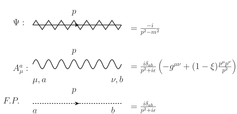
Figure 1: Propagators for the Full Lagrangian

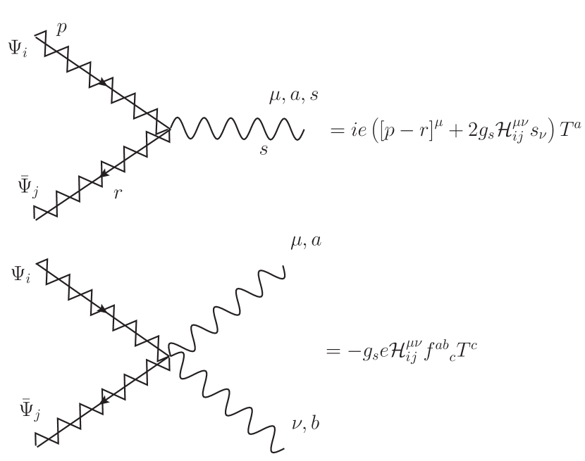
Figure 2: Interactions for $\Psi$, $\bar{\Psi}$ fields. All the particles left to the interaction vertex are incoming and all the particles right to the interaction vertex are outgoing.

Note that, for particles with integer spin, propagators serve just as an internal line. This is a consequence of anomalous relation between spin and statistics of the $\Psi$ fields for integer spin. Half integer fields may, however, appear as internal and external lines. Another interesting feature of this formulation is that the propagators of $\Psi$, and $\bar{\Psi}$ are of the Klein Gordon type which means that they do not carry any spin dependence. Still, the spin dependence in this formulation appears in the interaction term $\sim\mathcal{H}^{\mu\nu}$. For the case of spin one half it remains to be investigated in a beyond tree level calculation, whether this leads to some measurable difference with respect to the Dirac action. A further peculiarity of those Feynman rules is that the quartic interaction is antisymmetric under the interchange of $\mu$ and $\nu$ indices, and it is also antisymmetric under the interchange of $a$ and $b$ indices, so permuting gauge fields does not change the sign of the vertex. The interchange of fields $\bar{\Psi}$ and $\Psi$ does not affect the global sign of the coupling. Note that this applies to the cubic interaction too. Feynman rules of interactions of $\Psi$ and $\bar{\Psi}$ have spin dependence only given in the $\mathcal{H}^{\mu\nu}$ matrix. For sake of completeness, Feynman rules for gauge and Fadeev-Popov ghosts are derived and they are shown in figure 3.

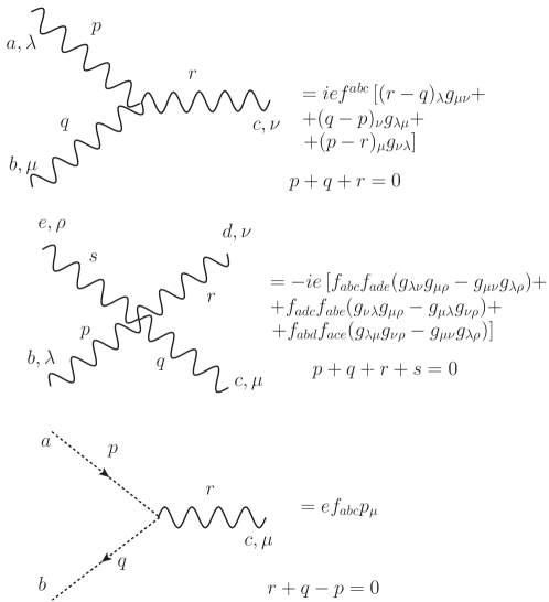
Figure 3: Interactions for $A_{\mu}^{a}$ and $\eta$ fields. Here the convention is that all the particles are incoming.

The simplicity of the toy Lagrangian (1) has its price.

• As it has been seen from the quantization section (V.2) the bosonic fields are obliged to be ghost fields due to their anti-commuting statistics.

• One would have to perform further checks of the type of Buchdahl:1958xv ; Velo:1970ur ; Buchdahl:1982ni in order to see whether the coupling to external gauge fields leads to inconsistencies. Even if there are no further problems with the coupling to standard gauge fields, the coupling of this model to gravity will most certainly lead to the type of inconsistencies described in Deser:2001dt .

• If one restricts to equations involving field strengths or “minimal fields” the much more general formulation of Siegel:1986de ; Siegel:1986zi ; Siegel:1988yz also takes an extremely simple form (after eliminating the auxiliary fields). However, when going beyond tree level, such reduced formulations (like the one presented here), are expected to lead to further problems with ghost fields at the loop level .

VI Conclusions

We report on an extended student project where a generic Lagrangian (1) and a generic Lorentz transformation (5) is investigated (similar to previous studies Koch:2011hc ). This Lagrangian allows to obtain the Klein-Gordon equation, the Dirac equation, and the Proca equations as special cases. The choice of which theory one wants to get is done by fixing a linear operator (3) to a special representation of SU(2) and by identifying the fields $\Omega$ and $\psi$ according to this choice. It is found that for arbitrary spin $s>0$, the resulting equations of motion are identical to the equations derived in Hurley:1972ju . The main advantage of the Lagrangian (1) is its simple form which allows to introduce and to study simultaneously field equations and fundamental quantum field theoretical concepts for various spin without overly heavy or abstract mathematical constructions.

In the discussion, various aspects of the model are explored: Local and global symmetries of the Lagrangian are discussed and the conserved currents are calculated. After this, the model is used in order to construct a simple Lagrangian which is invariant under transformations between spin zero fields $\Psi_{a},\,\Psi_{v}$ and spin one half partner fields ($\psi$, $\Omega$). It is also shown that this symmetry between free fields of different spin can be generalized to a symmetry between spin $s$ fields $\Psi_{a},\,\Psi_{b}$ and spin $2s+1/2$ partner fields $\psi$, $\Omega$.

Then, quantization in the free field case is reviewed. The discussion reveals that all fields, that are described by this Lagrangian have to obey Fermi statistics

$$\left[a(p,\sigma),a^{\dagger}(p^{\prime},\sigma^{\prime})\right]_{+} = (2\pi)^{3}2k_{0}\delta^{3}({\bf{p}-\bf{p^{\prime}}})\delta_{\sigma\sigma^{\prime}}\quad,$$ (105)

$$\left[b(p,\sigma),b^{\dagger}(p^{\prime},\sigma^{\prime})\right]_{+} = (2\pi)^{3}2k_{0}\delta^{3}({\bf{p}-\bf{p^{\prime}}})\delta_{\sigma\sigma^{\prime}}\quad.$$

This holds of course also for the spin zero and spin one fields discussed before. Thus, even though the equations of motion of this Lagrangian for the case of spin zero and spin one are the familiar ones, the quantized Lagrangian is fundamentally different. After performing a number of consistency checks we conclude, by the virtue of the spin-statistics theorem, that in this Lagrangian the fields with spin $0,1,2,\dots$ are necessarily ghost fields. On the other hand, this proof also shows that physical fermionic fields are well described within this model. Finally, based on this consistent quantization, the Feynman rules for the matter fields with arbitrary spin are written down and further issues are pointed out .

Many thanks to M.A. Diaz, M. Bañados, C. Valenzuela, and the Atlas-Andino group for valuable hints and discussions. The work of B. K. was supported by CONICYT project PBCTNRO PSD-73 and FONDECYT project 1120360. The work of N. R. was supported by CONICYT scholarship.

VII Appendix

VII.1 Proof of the field normalization

For all $j,k:-s\dots s$, we seek to solve a system of equations that contains

$$\bar{\nu}_{j}\nu_{k} = \pm\delta_{jk},$$ (106)

$$\bar{u}_{j}u_{k} = \delta_{jk}$$ (107)

$$u^{\dagger}_{j}\nu_{k} = 0$$ (108)

$$\nu^{\dagger}_{j}u_{k} = 0$$ (109)

$$\bar{u}_{j}\nu_{k} = 0$$ (110)

$$\bar{\nu}_{j}u_{k} = 0\quad.$$ (111)

The positive quantities $u^{\dagger}_{j}u_{k}$ and $\nu^{\dagger}_{j}\nu_{k}$ are possibly dependent on their Lorentz frame. We assume that they agree in the rest frame with the absolute value of the corresponding Lorentz invariant quantities

$$u^{\dagger}_{j}u_{k}|_{rest} = \delta_{jk}$$ (112)

$$\nu^{\dagger}_{j}\nu_{k}|_{rest} = \delta_{jk}\quad.$$ (113)

The $8(2s+1)^{2}$ equations (106-113) allow to determine the complex “vectors” $u_{j}=(a_{uj};b_{uj})$ and $\nu=(a_{\nu j};b_{\nu j})$, where the $a_{uj},b_{uj},a_{\nu j},b_{\nu j}$ have $2s+1$ complex components and $u_{j},\nu_{j}$ have $2(2s+1)$ complex components.

Without loss of generality one can make the choice

$$\nu_{1}=(a_{\nu 1},0,\dots;b_{\nu 1},0,\dots), \nu_{2}=(0,a_{\nu 2},\dots;0,b_{\nu 2},\dots), \dots$$ (114)

$$u_{1}=(a_{u1},0,\dots;b_{u1},0,\dots), u_{2}=(0,a_{u2},\dots;0,b_{u2},\dots), \dots$$ (115)

one observes that now most of the $8(2s+1)^{2}$ equations (106-113) are solved, leaving us with only eight diagonal equations $j=k$ for revery single spin state $j$.

$$\bar{\nu}_{j}\nu_{j} = \pm 1,$$ (116)

$$\bar{u}_{j}u_{j} = 1$$ (117)

$$u^{\dagger}_{j}\nu_{j} = 0$$ (118)

$$\nu^{\dagger}_{j}u_{j} = 0$$ (119)

$$\bar{u}_{j}\nu_{j} = 0$$ (120)

$$\bar{\nu}_{j}u_{j} = 0$$ (121)

$$u^{\dagger}_{j}u_{j}|_{rest} = 1$$ (122)

$$\nu^{\dagger}_{j}\nu_{j}|_{rest} = 1\quad.$$ (123)

This system has no solution for $\bar{\nu}_{j}\nu_{j}=+1$. In contrast it is solvable for $\bar{\nu}_{j}\nu_{j}=-1$ giving

$$\nu_{1}=\frac{1}{\sqrt{2}}(-1,0,\dots;1,0,\dots), \nu_{2}=\frac{1}{\sqrt{2}}(0,-1,\dots;0,1,\dots), \dots$$ (124)

$$u_{1}=\frac{1}{\sqrt{2}}(1,0,\dots;1,0,\dots), u_{2}=\frac{1}{\sqrt{2}}(0,1,\dots;0,1,\dots), \dots$$ (125)

The result holds in the rest frame. Since a Lorentz boost can not change the sign of a normalization and since $\bar{\nu}_{j}\nu_{j}$ is Lorentz invariant, it holds in any Lorentz frame. This proves that $\bar{\nu}_{j}\nu_{k}=-\delta_{jk}$ is the only possible field normalization.

VII.2 Completeness relations for $u$ and $\nu$

As one can note also in the section V.1 these spinors are normalized respect to the adjoint spinors $\bar{u}$ and $\bar{v}$ in any reference frame. Nevertheless, they are normalized with the respective hermitian transpose just in the restframe. This is because we want to measure a positive definite probability density in the particle restframe. Combining these two facts, one has in the particle restframe:

$$\bar{u}_{\sigma}u_{\sigma} = 1$$ (126)

$$u^{\dagger}_{\sigma}(0)u_{\sigma}(0) = 1=\bar{u}_{\sigma}u_{\sigma}$$ (127)

$$\bar{\nu}_{\sigma}\nu_{\sigma} = -1$$ (128)

$$\nu^{\dagger}_{\sigma}(0)\nu_{\sigma}(0) = 1=\bar{\nu}_{\sigma}\nu_{\sigma}$$ (129)

Note that the sum convention is used in equations (126) and (128), for spinor index $\sigma$. Using the definition of the adjoint spinors $\bar{u}_{\sigma}=u^{\dagger}_{\sigma}\gamma_{0}$ and $\bar{v}_{\sigma}=v^{\dagger}_{\sigma}\gamma_{0}$, one can split above equations

$$u^{\dagger}_{\sigma}(0)(\gamma_{0}-\openone)u_{\sigma}(0) = 0$$ (130)

$$\nu^{\dagger}_{\sigma}(0)(\gamma_{0}+\openone)\nu_{\sigma}(0) = 0\quad.$$ (131)

Now, the spinor basis for $u$ and $v$ is chosen such they are eigenvectors of $\gamma_{0}$ with $\pm 1$ eigenvalues respectively. This implies that

$$(\gamma_{0}-\openone)u_{\sigma} = 0$$ (132)

$$u_{\sigma}^{\dagger}(\gamma_{0}-\openone) = \bar{u}_{\sigma}(\openone-\gamma_{0})=0\Rightarrow$$

$$u_{\sigma}\bar{u}_{\sigma}\gamma_{0} = u_{\sigma}\bar{u}_{\sigma}$$ (133)

$$\gamma_{0}u_{\sigma}\bar{u}_{\sigma} = u_{\sigma}\bar{u}_{\sigma}\Rightarrow$$ (134)

$$u_{\sigma}\bar{u}_{\sigma}\gamma_{0} = \gamma_{0}u_{\sigma}\bar{u}_{\sigma}=u_{\sigma}\bar{u}_{\sigma}$$ (135)

That means in the particle restframe, the projector $u_{\sigma}\bar{u}_{\sigma}$, commute with $\gamma_{0}$, in other words it can be only a linear combination of $\gamma_{0}$ and the identity into this frame. So, one gets the ansatz

$$u_{\sigma}\bar{u}_{\sigma} = A\gamma_{0}+B\openone$$

$$u_{\sigma}\bar{u}_{\sigma}u_{\sigma} = u_{\sigma}=A\gamma_{0}u_{\sigma}+Bu_{\sigma}=(A+B)u_{\sigma}\Rightarrow$$

$$(A+B) = 1$$ (136)

By other hand, one gets:

$$u_{\sigma}\bar{u}_{\sigma}u_{\sigma}\bar{u}_{\sigma} = (A\gamma_{0}+B\openone)^{2}=u_{\sigma}\bar{u}_{\sigma}=(A\gamma_{0}+B\openone)\Rightarrow$$ (137)

$$A^{2}+B^{2} = B$$

$$2AB = A$$ (138)

So one have a system of two equations plus an identity, which is fullfilled by $A=B=1/2$. So one gets in the restframe:

$$u_{\sigma}(0)\bar{u}_{\sigma}(0) = \frac{1}{2}\left(\gamma_{0}+\openone\right)$$ (139)

$$v_{\sigma}(0)\bar{v}_{\sigma}(0) = \frac{1}{2}\left(\gamma_{0}-\openone\right)$$ (140)

Finally, in order to generalize relation to any frame with 3-momentum $p_{k}$ and energy $E$, one has to perform a Lorentz boost. It is easy to see that from the equations below that a Lorentz boost over $u_{\sigma}$ and $\bar{u}_{\sigma}$ spinors is given by

$$u_{\sigma}(p) = \left(\begin{array}[]{cc}\exp\frac{1}{2}\beta_{k}\Sigma^{k}&0\\ 0&\exp\frac{-1}{2}\beta_{k}\Sigma^{k}\end{array}\right)u_{\sigma}(0)$$ (144)

$$\bar{u}_{\sigma}(p) = \bar{u}_{\sigma}(0)\left(\begin{array}[]{cc}\exp\frac{-1}{2}\beta_{k}\Sigma^{k}&0\\ 0&\exp\frac{1}{2}\beta_{k}\Sigma^{k}\end{array}\right)$$ (147)

and they are a generalization for the equations (5) for $\psi$, $\Omega$ spinors. Thus

$$u_{\sigma}(p)\bar{u}_{\sigma}(p) = \left(\begin{array}[]{cc}\exp\frac{1}{2}\beta_{k}\Sigma^{k}&0\\ 0&\exp\frac{-1}{2}\beta_{k}\Sigma^{k}\end{array}\right)u_{\sigma}(0)\bar{u}_{\sigma}(0)\left(\begin{array}[]{cc}\exp\frac{-1}{2}\beta_{k}\Sigma^{k}&0\\ 0&\exp\frac{1}{2}\beta_{k}\Sigma^{k}\end{array}\right)$$ (152)

$$= \frac{1}{2}\left\{\left(\begin{array}[]{cc}\exp(\frac{1}{2}\beta_{k}\Sigma^{k})\exp(\frac{-1}{2}\beta_{l}\Sigma^{l})&0\\ 0&\exp(\frac{-1}{2}\beta_{k}\Sigma^{k})\exp(\frac{1}{2}\beta_{l}\Sigma^{l})\end{array}\right)\right.$$ (158)

$$\;\;+\left.\left(\begin{array}[]{cc}0&\exp(\frac{1}{2}\beta_{k}\Sigma^{k})\exp(\frac{1}{2}\beta_{l}\Sigma^{l})\\ \exp(\frac{-1}{2}\beta_{k}\Sigma^{k})\exp(\frac{-1}{2}\beta_{l}\Sigma^{l})&0\end{array}\right)\right\}$$

The way how this expression can be further simplified depends on the choice of the representation $\Sigma_{i}$. Therefore we give the explicit form for the cases discussed in this paper.

• If the representation $\Sigma_{i}$ fulfills a Clifford algebra

  $$\{\Sigma_{i},\Sigma_{j}\}=2\delta_{ij}\openone\quad,$$ (159)

  like it is the case for spin $\Sigma_{i}=\sigma_{i}$. One finds with $\beta_{i}=\beta n_{i}$

  $$u_{\sigma}(p)\bar{u}_{\sigma}(p) = \frac{1}{2}\left\{\left(\begin{array}[]{cc}\openone&0\\ 0&\openone\end{array}\right)+\left(\begin{array}[]{cc}0&\openone\cosh(\beta)+n_{i}\sigma^{i}\sinh(\beta)\\ \openone\cosh(\beta)-n_{i}\sigma^{i}\sinh(\beta)&0\end{array}\right)\right\}$$ (164)

  and

  $$\nu_{\sigma}(p)\bar{\nu}_{\sigma}(p) = \frac{-1}{2}\left\{\left(\begin{array}[]{cc}\openone&0\\ 0&\openone\end{array}\right)-\left(\begin{array}[]{cc}0&\openone\cosh(\beta)+n_{i}\sigma^{i}\sinh(\beta)\\ \openone\cosh(\beta)-n_{i}\sigma^{i}\sinh(\beta)&0\end{array}\right)\right\}$$ (169)

• For the adjoint representation $i\epsilon_{klm}$, which is used for spin one the corresponding algebra is

  $$\left\{i\epsilon_{i},i\epsilon_{j}\right\}_{km}=2\delta_{ij}\openone_{km}-\delta_{im}\delta_{jk}-\delta_{ik}\delta_{jm}\quad.$$ (170)

  This implies that the exponential can be expanded as

  $$\exp(i\theta n_{j}\epsilon_{j})_{km}=\openone_{km}\cosh(\theta)+in_{j}\epsilon_{jkm}\sinh(\theta)+n_{k}n_{m}(1-\cosh(\theta))\quad.$$ (171)

  With this the completeness relations for spin one read

  $$u_{\sigma}(p)\bar{u}_{\sigma}(p)|_{s=1}=\frac{1}{2}\left\{\left(\begin{array}[]{cc}\openone&0\\ 0&\openone\end{array}\right)\right.\quad\quad\quad\quad\quad\quad\quad\quad\quad\quad\quad\quad\quad\quad\quad\quad\quad\quad\quad\quad\quad\quad\quad\quad\quad\quad\quad\quad\quad\quad$$ (174)

  $$+\left.\left(\begin{array}[]{cc}0&\openone_{km}\cosh(\beta)+in_{j}\epsilon_{jkm}\sinh(\beta)-2n_{k}n_{m}\sinh^{2}(\beta/2)\\ \openone_{km}\cosh(\beta)-in_{j}\epsilon_{jkm}\sinh(\beta)-2n_{k}n_{m}\sinh^{2}(\beta/2)&0\end{array}\right)\right\}$$ (177)

  and

  $$\nu_{\sigma}(p)\bar{\nu}_{\sigma}(p)|_{s=1}=\frac{1}{2}\left\{\left(\begin{array}[]{cc}\openone&0\\ 0&\openone\end{array}\right)\right.\quad\quad\quad\quad\quad\quad\quad\quad\quad\quad\quad\quad\quad\quad\quad\quad\quad\quad\quad\quad\quad\quad\quad\quad\quad\quad\quad\quad\quad\quad$$ (180)

  $$-\left.\left(\begin{array}[]{cc}0&\openone_{km}\cosh(\beta)+in_{j}\epsilon_{jkm}\sinh(\beta)-2n_{k}n_{m}\sinh^{2}(\beta/2)\\ \openone_{km}\cosh(\beta)-in_{j}\epsilon_{jkm}\sinh(\beta)-2n_{k}n_{m}\sinh^{2}(\beta/2)&0\end{array}\right)\right\}$$ (183)

  The relations (174, 180) contain an extra term $\sim n_{k}n_{m}$ which potentially causes problems when causal propagation is studied. Whether those problems can be solved or whether they are related to the known causality problems in spin one field equations Velo:1970ur remains to be seen.

The completeness relations (164, 169) are used when studying causality in the section V.1.

References

- (1) P. A. M. Dirac, Proc. Roy. Soc. Lond. 155A, 447-459 (1936).
- (2) M. Fierz, W. Pauli, Proc. Roy. Soc. Lond. A173, 211-232 (1939).
- (3) I.M. Gel’fand and A.M. Yaglom, Sov. Journ. JETP 18, 703 (1948).
- (4) V. Bargmann and E. P. Wigner, Proc. Nat. Acad. Sci. 34, 211 (1948).
- (5) S. Weinberg, Phys. Rev. 133, B1318 (1964).
- (6) S. J. Chang, Phys. Rev. 161, 1308-1315 (1967).
- (7) W. K. Tung, Phys. Rev. 156, 1385 (1967).
- (8) C. R. Hagen, W. J. Hurley, Phys. Rev. Lett. 24, 1381-1384 (1970).
- (9) W. J. Hurley, Phys. Rev. D3, 2339-2347 (1971).
- (10) W. J. Hurley, Phys. Rev. D4, 3605-3616 (1971).
- (11) L. P. S. Singh, C. R. Hagen, Phys. Rev. D9, 898-909 (1974).
- (12) L. P. S. Singh, C. R. Hagen, Phys. Rev. D9, 910-920 (1974).
- (13) V. D. Gershun and V. I. Tkach, JETP Lett. 29, 288 (1979) [Pisma Zh. Eksp. Teor. Fiz. 29, 320 (1979)].
- (14) F. A. Berends, G. J. H. Burgers, H. van Dam, Nucl. Phys. B271, 429 (1986).
- (15) W. Siegel, Nucl. Phys. B 284, 632 (1987).
- (16) W. Siegel and B. Zwiebach, Nucl. Phys. B 282, 125 (1987).
- (17) P. S. Howe, S. Penati, M. Pernici, P. K. Townsend, Phys. Lett. B215, 555 (1988).
- (18) W. Siegel, hep-th/0107094.
- (19) N. Berkovits, Phys. Lett. B 388, 743 (1996) [hep-th/9607070].
- (20) R. R. Metsaev, [hep-th/9810231].
- (21) D. Francia and A. Sagnotti, Phys. Lett. B 543, 303 (2002) [hep-th/0207002].
- (22) J. Niederle, A. G. Nikitin, Phys. Rev. D64, 125013 (2001). [hep-th/0412213].
- (23) M. A. Vasiliev, Fortsch. Phys. 52, 702 (2004) [arXiv:hep-th/0401177].
- (24) G. Savvidy, Fortsch. Phys. 54, 472 (2006) [hep-th/0512012].
- (25) X. Bekaert, N. Boulanger, S. Cnockaert and S. Leclercq, Fortsch. Phys. 54, 282 (2006) [hep-th/0602092].
- (26) D. Francia, Nucl. Phys. B 796, 77 (2008) [arXiv:0710.5378 [hep-th]].
- (27) D. Francia, Fortsch. Phys. 56, 800 (2008) [arXiv:0804.2857 [hep-th]].
- (28) J. Engquist and O. Hohm, Fortsch. Phys. 56, 895 (2008) [arXiv:0804.2627 [hep-th]].
- (29) A. Campoleoni, D. Francia, J. Mourad and A. Sagnotti, Nucl. Phys. B 815, 289 (2009) [arXiv:0810.4350 [hep-th]].
- (30) A. K. H. Bengtsson, Fortsch. Phys. 57, 499 (2009) [arXiv:0902.3915 [hep-th]].
- (31) I. L. Buchbinder, V. A. Krykhtin and L. L. Ryskina, Nucl. Phys. B 819, 453 (2009) [arXiv:0902.1471 [hep-th]].
- (32) R. Manvelyan, K. Mkrtchyan and W. Ruhl, Nucl. Phys. B 836, 204 (2010) [arXiv:1003.2877 [hep-th]].
- (33) A. Campoleoni, S. Fredenhagen and S. Pfenninger, JHEP 1109, 113 (2011) [arXiv:1107.0290 [hep-th]].
- (34) D. Polyakov, Phys. Rev. D 84, 126004 (2011) [arXiv:1106.1558 [hep-th]].
- (35) D. Chicherin, S. Derkachov, D. Karakhanyan and R. Kirschner, Nucl. Phys. B 854, 393 (2012) [arXiv:1106.4991 [hep-th]].
- (36) M. Montero and E. Martin-Martinez, Phys. Rev. A 84, 012337 (2011) [arXiv:1105.0894 [quant-ph]].
- (37) H. A. Buchdahl, Nuovo Cim. 10, 96-103 (1958).
- (38) G. Velo, D. Zwanziger, Phys. Rev. 188, 2218-2222 (1969).
- (39) H. A. Buchdahl, J. Phys. A A15, 1057-1062 (1982).
- (40) R. Illge, R. Schimming, Annalen Phys. 8, 319-329 (1999).
- (41) R. Illge, Exp. Tech. Phys. 34, 429-432 (1986).
- (42) R. Illge, Comm. Math. Phys. 158, 433-457 (1993).
- (43) S. Deser and A. Waldron, Nucl. Phys. B 631, 369 (2002) [arXiv:hep-th/0112182].
- (44) D. Sorokin, AIP Conf. Proc. 767, 172-202 (2005). [hep-th/0405069].
- (45) A. Zecca, Int. Jour. Th. Phys. 46. 1045-1054. (2007).
- (46) V. I. Belinicher, Teor. Mat. Fiz. 20, 320-337 (1974).
- (47) H. S. Green, Austral. J. Phys. 31, 219 (1978).
- (48) I. L. Buchbinder, A. V. Galajinsky and V. A. Krykhtin, Nucl. Phys. B 779, 155 (2007) [hep-th/0702161].
- (49) I. L. Buchbinder and A. V. Galajinsky, JHEP 0811, 081 (2008) [arXiv:0810.2852 [hep-th]].
- (50) F. J. Belinfante, Phys. Rev. 92, 997-1001 (1953).
- (51) L. M. Brown, Phys. Rev. 111, 957 (1958).
- (52) R.P. Feynman and M. Gell-Mann, Phys. Rev. 109, 193 (1958);
- (53) A. Proca, Compt. Rend. 202, 1420 (1936).
- (54) W. Rarita and J. Schwinger, Phys. Rev. 60, 61 (1941).
- (55) B. Koch and N. Rojas, arXiv:1101.4619 [hep-th].