Oscillatons
Abstract
We solve numerically the Einstein-Klein-Gordon system with spherical symmetry, for a massive real scalar field endowed with a quartic self-interaction potential, and obtain the so-called -oscillatons which is the short name for oscillating soliton stars. We analyze numerically the stability of such oscillatons, and study the influence of the quartic potential on the behavior of both, the stable (S-oscillatons) and unstable (U-oscillatons) cases under small and strong radial perturbations.
pacs:
04.40.-b,04.25.D-,95.30.Sf,95.35.+dI Introduction
Oscillatons are non-singular and asymptotically flat solutions of the Einstein-Klein-Gordon (EKG) equations, in which both metric and scalar field are fully time-dependentSeidel and Suen (1991); Urena-Lopez et al. (2002); Alcubierre et al. (2003); Urena-Lopez (2002); Balakrishna et al. (2008). They can be considered as gravitationally bounded objects made of a real scalar field in the classical regime, and were first discovered by Seidel and SuenSeidel and Suen (1991). Oscillatons should be distinguished from their complex counterparts, the so-called boson stars, for which the space-time geometry remains staticSeidel and Suen (1994); Balakrishna et al. (2006); Colpi et al. (1986); Guzman (2004). In the literature we can find other works describing these bound objects and their stability propertiesGrandclement et al. (2011); Fodor et al. (2010, 2010); Masso et al. (2005); Obregon et al. (2005); Matos et al. (2008); Page (2004). Also there have been many works about numerical evolution of scalar fiels in different cosmological and astrophysical contextGuzman and Rueda-Becerril (2009); Bernal and Siddhartha Guzman (2006); Bernal and Guzman (2006).
Ref. Alcubierre et al. (2003) presented an exhaustive study of oscillatons for the simplest case of a massive, non-self interacting, scalar field. It is shown in there that, as in the case of boson stars, oscillatons can be classified into stable (S-branch) and unstable (U-branch) configurations. S-oscillatons are stable configurations under small radial perturbations, and they typically migrate to other S-profiles if strongly perturbed. On the other hand, U-oscillatons are intrinsically unstable: they migrate to the S-branch if their mass is moderate, but they may collapse into black holes if their mass is large enough.
The case of oscillatons with a self-interaction term in the scalar field potential remains without study. This is in contrast to the case of boson stars, whose properties are well known even in the self-interacting caseColpi et al. (1986); Balakrishna et al. (1998); Guzman (2004); Balakrishna et al. (1998). It is the main purpose of this paper to cover this omission, and to study the properties of self-interacting oscillatons. For that we make use of techniques and methods that parallel those used in boson star studies and for non-interacting oscillatonsSeidel and Suen (1990); Balakrishna et al. (1998); Alcubierre et al. (2003), which will ease the comparison between the two types of scalar objects.
A summary of the paper is as follows. In Sec. II, we present the equations motion of the self-interacing scalar field. In Sec. III we show the resuls of the equilibrium configuration and their representative properties, for different values of the self-interaction parameter. In Sec. IV we present the results of the dynamical evolution of oscillatons, and the separate analysis of (stable) S-oscillatons and (unstable) U-oscillatons. Finally, Sec. V is devoted to overall conclusions.
II Mathematical Background
The action that describes our self-gravitating system is
| (1) |
where is the scalar potential,
| (2) |
denotes the mass of the scalar field, and is the quartic interaction parameter. We shall be interested in the spherically symmetric case for which the metric is written as
| (3) |
where is the radial function, and is the lapse function.
II.1 Evolution Equations
The energy-momentum tensor for the scalar field endowed with a scalar field potential is defined as
| (4) |
We can identify the Klein-Gordon (KG) equation with the conservation equations of the scalar field energy-momentum tensor,
| (5) |
where is the d’Alembertian operator. Following Ref. Alcubierre et al. (2003), we introduce the first order variables
| (6) |
in order to write appropriate evolution equations for the scalar fields. Hereafter, a prime denotes derivative with respect to , and a dot denotes derivative with respect to . The KG equation is then represented by the following set of first order differential equations
| (7a) | |||||
| (7b) | |||||
| (7c) | |||||
As for the metric functions, we will use the so-called Hamiltonian constraint for the radial function,
| (8) |
and the polar-areal slicing condition for the lapse function,
| (9) |
For numerical purposes, in all the above equations, we have introduced the dimensionless quantities , , , and . Eqs. (7-9) are the total set of evolution equations we shall use to explore the properties of self-interacting oscillatons.
III Equilibrium Configuration
Before we evolve the EKG equations, we turn our attention to equilibrium configurations of the self-interacting oscillatons. For that, we consider momentarily a different set of variables: , and . In terms of these variables, the Einstein equations, , read
| (10a) | |||||
| (10b) | |||||
| (10c) | |||||
whereas the KG is the single equation
| (11) | |||||
The above equations will be solved by introducing in Eqs. (10) and (11), the following Fourier expansions for the scalar field and the metric functions,
| (12a) | |||||
| (12b) | |||||
| (12c) | |||||
where is called the fundamental frequency, and is the mode at which the Fourier series are truncated. We define , with .
After some lengthy but straightforward algebra, we obtain first-order differential equations for the coefficients , , and , where . This system of equations can be solve with the aid of an integrator, like odeint, that uses an adaptive step-size control which allows us to achieve some predetermined accuracy in the solution with minimum computational effort (see Wiliam H. Press and others. (1992)). We also use a second order Runge-Kutta method (RK2) in order to verify the convergence of our code, since this method uses a fix step-size. Once the profiles of and are known, we will get the subsequent values of , for , from the algebraic restriction (10a).
III.1 Boundary Conditions
Appropriate boundary conditions can be obtained by analyzing the regularity of the functions , , and at . First, we realize that , which implies , and for . Second, we find that , so that .
From asymptotic flatness, we know that , which leads to , and for . The scalar field must vanish when , and this implies . Likewise, we expect , and then , whereas for . Actually, the fundamental frequency is always an output value obtained after the solution of Eqs. (10b), (10c), and 11).
Note that there are not boundary conditions for and at . We need to find these values in such manner that all boundary conditions at are satisfied. For each solution, we will fix the value of the first scalar Fourier coefficient , and adjust the rest of the coefficients and until we satisfy the boundary conditionsUrena-Lopez et al. (2002); we use a non-linear shooting method to find these values. Thus, we obtain a set of eigenvalues for each value , which in turn defines uniquely a given configuration.
III.2 Numerical Results
We truncate the Fourier expansions (12) at . Then, according to what we said about boundary conditions, we need to calculate the value of the coefficients , , , and , for each value of the parameter. Table 1 contains the values obtained once the boundary conditions were satisfied at for the fixed value ..
| 0.0 | 1.0 | 2.0 | 3.0 | |
|---|---|---|---|---|
| 8.98e-01 | 8.91e-01 | 8.88e-01 | 8.84e-01 | |
| 6.90e-05 | 1.16e-05 | 1.36e-05 | 3.54e-05 | |
| 2.66e-06 | 7.32e-06 | 9.11e-06 | 1.68e-05 | |
| 5.77e-07 | 3.69e-06 | 6.85e-06 | 6.57e-07 |
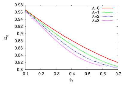
In contrast to the non-interacting case, the increasing of complicates the solution of the equations of motion as we consider larger values of . As a consequence, in Fig. 2 we observe that, for , we were able to compute the values of masses and frequencies for scalar field values up to , whereas for we could compute up to . In the same way, as the values of and of are increased, we must decrease the size of the numerical domain, represented by .
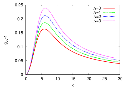
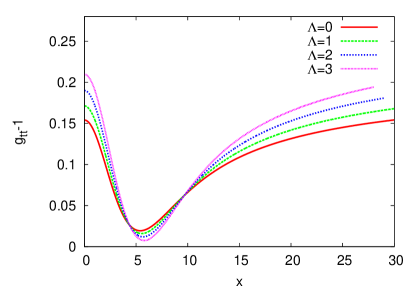
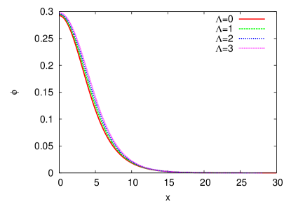
We present in Fig. 1 the results for the metric functions , , and the scalar field , for configurations with and . This functions were calculated for different values of the parameter . Note that the metric functions are non-singular at the origin and asymptotically flat for large .
Following Urena-Lopez et al. (2002), the total mass is calculated by the so-called Schwarzschild mass,
| (13) |
and the fundamental frequency is obtained from
| (14) |
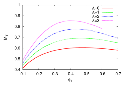
In Fig. 2, we show the values obtained for the total masses and fundamental frequencies as functions of the central value of the first scalar field (Fourier) coefficient and for different values of . We can see that the mass of a given configuration increases for larger values of increases, whereas the fundamental frequency decreases.
In Table 2, we show the values of the fundamental frequency and of the critical masses for each value of . The critical mass is defined as the maximum mass attained by an equilibrium configuration; this maximum can be seen in Fig. 2 for each value of .
| () | |||
|---|---|---|---|
| 0.0 | 0.605 | 0.48 | 0.862 |
| 1.0 | 0.694 | 0.47 | 0.851 |
| 2.0 | 0.770 | 0.44 | 0.850 |
| 3.0 | 0.854 | 0.39 | 0.848 |
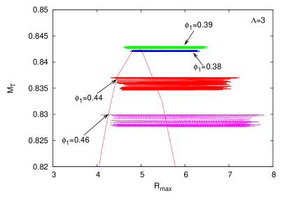
For completeness, we show in Fig. 3, for different equilibrium configurations, the critical mass as a function of the radius at which the metric radial function reaches its maximum value at .

IV Numerical Evolution of self-interacting oscillatons
We proceed now to the evolution of the EKG equations using the method of lines. For the time integrations, we use a fourth order Runge-Kutta method (RK4), and second order centered differences to discreticize spatial derivatives. A second-order Runge-Kutta method (RK2) is used for the spatial integration of the metric functions at each time level. Special care is needed for Eq. (7b), otherwise its discretization would not be second-order accurate because of the presence of the factor in the principal part. The transformation that guarantees the accuracy of our simulations at the origin is
| (15) |
IV.1 Boundary Conditions
To properly account for the origin at , we use the fictitious point as in Alcubierre et al. (2003), and take a spatial grid of the form . From the evolution equation of , Eq. (7a), we can see that it not necessary to apply boundary condition for , because the evolution equation can be integrated all the way from the boundary point up to the outer boundary point. This is possible since the evolution equation (7a) does not have spatial derivatives. Likewise, we use the fictitious point to impose appropriate parity conditions on the scalar field variables: is even, and is odd.
At the outer numerical boundary, we assume that behaves as an outgoing wave pulse of the form
| (16) |
where is an arbitrary function. In differential form, Eq. (16) becomes
| (17) |
By using finite difference in Eq. (17), we can solve it to find the unknown boundary value at the new time level. Because behaves as an outgoing wave at the boundary, so does . Then, the outgoing wave boundary condition applied to implies that at the outer boundary
| (18) |
We used this expression to obtain boundary values for after the calculation of those of and .
Boundary conditions for the metric functions are the following. Local flatness at the origin implies that and , and these two conditions together imply that . We use these two values at the first and second grid points to integrate the second order Hamiltonian constrain outwards to obtain .
As for the lapse function, we impose as an outer boundary condition; this is because in vacuum our slicing condition implies that we are in Schwarzschild coordinates. Then, we are assuming that our boundary conditions are sufficiently far away as to be always in vacuum. Finally, the slicing condition is integrated inwards to obtain the full profile of .
IV.2 Initial Conditions
For most of our numerical experiments, we consider as initial conditions the equilibrium configurations calculated in Sec. III; hence,
| (19) | |||||
| (20) | |||||
| (21) |
Our interest resides mainly in the equilibrium properties of these configurations, and it is first necessary to develop different analysis techniques for their study. In this we will include, to begin with, initial configurations that are a deformation of the original equilibrium ones. There is a practical reason behind: equilibrium configurations are easy to evolve, whereas general configurations may be very difficult to follow as they develop in time.
IV.3 Numerical Results
We start by calculating some properties of the equilibrium configurations found now by the evolution code. For instance, the critical mass of self-interacting oscillatons, for different values of , are shown in Table 3.
| () | ||
|---|---|---|
| 0.0 | 0.599 | 0.47 |
| 1.0 | 0.686 | 0.46 |
| 2.0 | 0.767 | 0.42 |
| 3.0 | 0.843 | 0.39 |
The total mass was obtained through the integration of the energy density calculated from the time-time component of the scalar field stress-energy tensor, . Because of the spherical symmetry, this method gives identical results to the Schwarzschild mass in Eq. (13). We notice a little discrepancy with respect to the values reported in Sec. III, this is because of the evolution code is more accurate and does not depend upon the truncation we had to impose upon the Fourier expansions in (12).
IV.3.1 Code tests
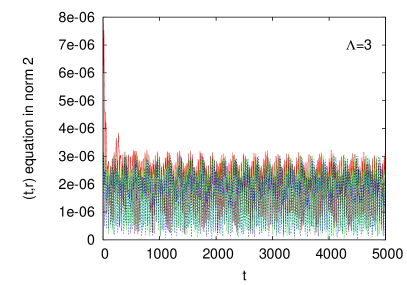
To revise the accuracy of our numerical calculations, we monitored the momentum constraint (10a),
| (22) |
and calculated the -norm of the value of across the grid as a function of time using three different spatial grid sizes, see Fig. 4. It can be seen that the accuracy of the numerical code is not altered by the values of the quartic parameter .
On the other hand, Fig. 5 shows the mass-differential function for a run with a numerical boundary located at , and for . We can see that the plots are practically the same up to , but differ one from each other at the outer parts of the numerical domain. These discrepancies, of the order of , arise because part of scalar field has been reflected from the outer boundary. The error is not significant and we were able to keep it under control during the numerical evolution.
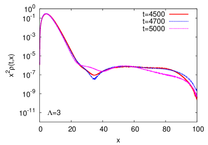
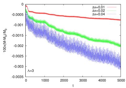
Fig. 6 shows the evolution of the total integrated mass for each time level. We can observe a small adjustment of the original mass, because there is a small ejection of scalar field at the beginning of the run. We can notice a steady decay of the mass, which is evidence of an intrinsic dissipation of our numeric code; it can be reduced by taking a finer spatial grid, and then it cannot be considered an intrinsic decay of the oscillatons.
IV.3.2 S-branch and Quasi-normal Modes
We present here numerical evidence that the characterization of stable, S-branch, and unstable, U-branch oscillatons is preserved in the case of the inclusion of a quartic interaction, much in the same manner as in the case of non self-interacting oscillatons and boson stars.
To begin with, we show in Fig. 7 the evolution of the maximum value of the radial metric function , corresponding to an equilibrium configuration with . The outer boundary of the numerical domain was set at , and the run was followed up to a time . It can be noticed that the configuration maintains the same oscillatory pattern at all times and for all values of . This is an evidence of the stability of the oscillations in response to small radial perturbations. In this case, the perturbations come from the truncation of the Fourier series (12) and the discretization error of the numerical solutions.
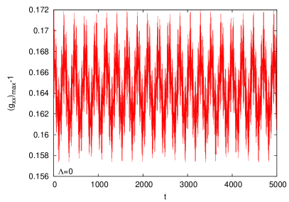
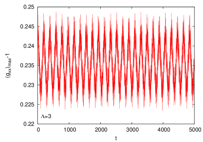
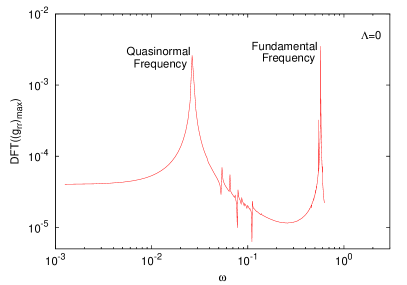
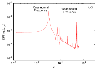
Fig. 8 presents the Fourier transform of the oscillations shown in Fig. 7; we observe that the maximum of the oscillates periodically with two distinctive time scales. The short-period oscillation (large frequency) corresponds to the fundamental frequency used in the Fourier expansions (12). The large-period oscillation (small frequency) is an overall vibration of the configuration that we identify as the characteristic quasi-normal modes of the oscillatons.
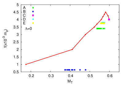
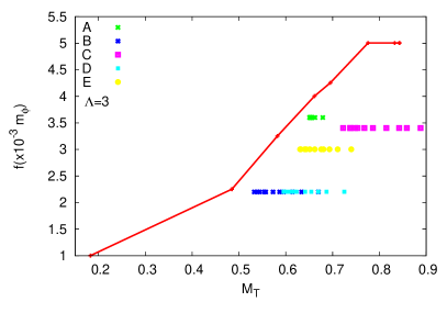
Following the analysis done in Alcubierre et al. (2003), we calculate the power spectrum of the evolution for the entire S-branch; we show in Fig. 9 the quasi-normal frequency as a function of the total mass . This kind of plots has proved useful in the analysis of the evolution of general scalar field configurations, seeSeidel and Suen (1990); Balakrishna et al. (1998); Alcubierre et al. (2003).
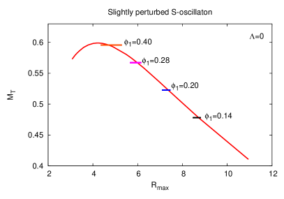
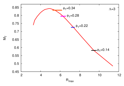
On the other hand, Fig. 10 presents the evolution of the total mass and ( is the value where the radial metric function reaches its maximum value) as compared with the values corresponding to equilibrium configurations. All the cases correspond to the S-branch.
It is observed that slightly perturbed S-oscillatons are not migrating to another S-oscillaton profile, but rather they oscillate with a small amplitude around the original equilibrium configuration. It is then concluded that S-oscillatons are stable under small radial perturbations, and that the frequencies show in Fig. 8 are their intrinsic quasi-normal modes.
IV.3.3 Perturbed S-oscillatons
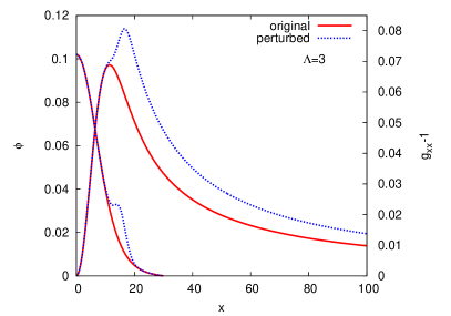
We now turn our attention to the evolution of some strongly-perturbed S-oscillatons. We use a Gaussian profile as a perturbation applied to the original equilibrium configurations; see Fig. 11 for an example of this perturbation in the case of an S-oscillaton with , so that its mass is increased by %. The purpose is to analyze whether S-oscillatons are stable under strong perturbations, and the conditions to be met for the collapse into a black hole.
First, we increased the original mass of the equilibrium configuration (see Fig. 2) with by % and % for all values. The initial masses for are () and . (), for are () and (), for are () and (), and for are () and ().
From Fig. 12 we can see that for the perturbed configuration with its mass increased by % collapses into a black hole, while for the rest of the values this configuration migrates to another oscillaton located on the S-branch. The reason for this is that the -configuration has an initial mass that is larger than the critical mass of equilibrium configurations (see Table 2), whereas for the other cases the initial mass is smaller than the critical one. The perturbed configurations with their mass increased by are able to migrate to another S-oscillaton.
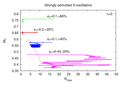
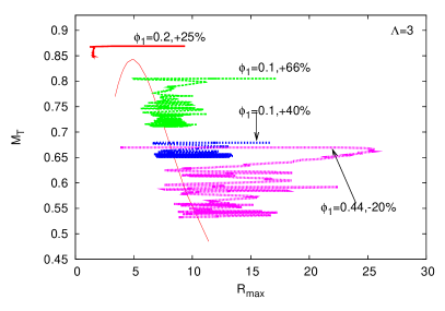
For equilibrium configurations with , we increased its original mass in obtaining the following initial masses: . (), . (), . (), and . (). This configuration collapses into a black hole for all values of ; in all cases, the initial mass of the perturbed configuration is larger than critical one corresponding to each case.
Finally, for equilibrium configurations with , we decreased its original mass by %: . (),. (), . (), and . (). As we can see in Fig. 12, these configurations lose mass until they reach the position of another S-oscillaton.
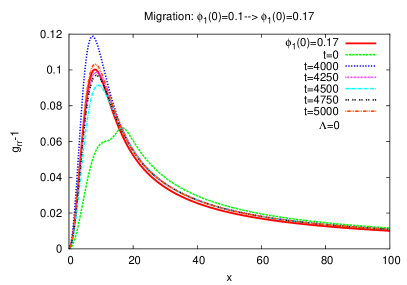
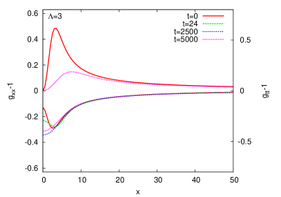
We have noticed that oscillatons maintain a fixed vibration frequency during its evolution. This is shown in Fig. 12, where we present the migration path of oscillatons with (with its mass increased by %), and with (with its mass decreased by %), which are labeled and in Fig. 9. We can appreciate that the perturbed oscillaton with () is migrating to an equilibrium configuration with . This can also can be seen in Fig. 13, which shows the profile of the metric coefficient rapidly approaching and oscillating around the final configuration.
Then, as reported in Ref. Alcubierre et al. (2003), we have found that strongly perturbed S-oscillaton are able to migrate to another S-oscillaton when their original mass is smaller than critical mass. But, if the original mass increases enough to be larger than the critical one, this perturbed configuration will collapse into a black hole, except in the case of diluted oscillatons, with low values of , in which the collapse to a black hole can be prevent by the gravitational cooling mechanism.
IV.3.4 U-branch
We identify as U-oscillatons the equilibrium configurations that are located on the right-hand side of the critical configuration in a plot of versus , see Fig. 2, or located on the left-hand side in a plot of versus , see Fig. 3. To evolve these equilibrium configurations, we also use the slightly-perturbed, by numerical inaccuracies, configurations, which in general decay and migrate to a configuration located on the S-branch.
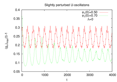
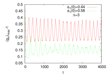
Fig. 14 shows some slightly perturbed U-oscillatons, and we can see that the equilibrium configuration is more unstable (the quicker it starts to migrate) for larger values of . This also can be seen in Fig. 15, where we show the evolution of the maximum value of the radial metric coefficient for the slightly perturbed configurations with central field values and .
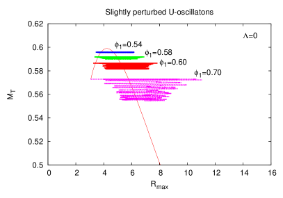
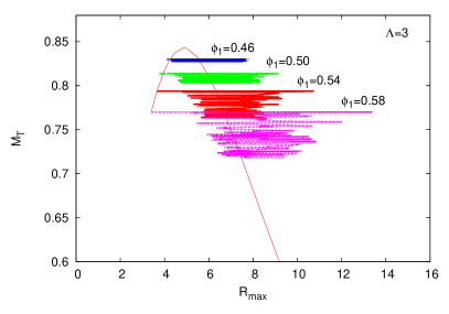
Thus, we confirm that the U-oscillatons are intrinsically unstable under small perturbation, they decay and migrate to the S-branch. In Fig. 9, we show the migration of the slightly perturbed U-oscillaton with and , labeled and for , labeled for and , and labeled for .
IV.3.5 Perturbed U-branch
We study now the behavior of the U-branch equilibrium configurations under strong perturbations. An example of the typical behaviors is provided by the configuration with for all values of . First, we increase its original mass by %; the resulting initial masses are: (), (), (), and ().
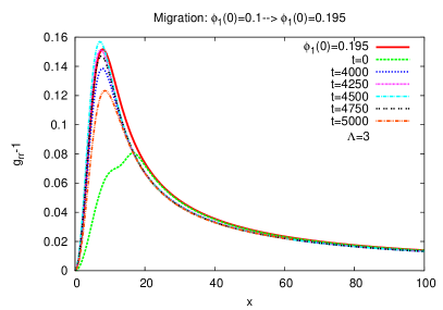
In the case of , this configuration collapses into a black hole, as reported also inAlcubierre et al. (2003). But, for other values, the same configuration is able to migrate to the S-branch, see Fig. 16. The migration path for this configuration is labeled as , for , in Fig. 9. In contrast, a mass increase by for the equilibrium configuration with provokes a rapid collapse into a black hole, independently of the value of .
In another experiment, we decrease the original mass of a -oscillaton by . The initial masses obtained are: . (), . (), . (), and . (). As expected, these perturbed U-oscillatons lose mass and migrate to the S-branch. The evolution of these strongly perturbed configurations appears in Fig. 16, and their path migration is labeled as in Fig. 9 for all the values of .
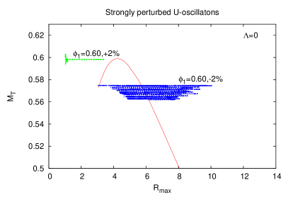
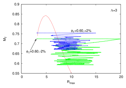
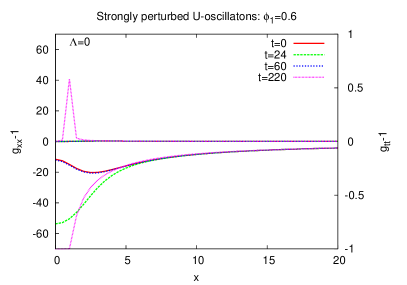
Fig. 17 shows the behavior of the metric functions and for the case of strongly perturbed U-oscillaton. In the plot for , we can see that shows the well known ”collapse of the lapse”, and shows the ”grid stretching”; both phenomena signal the possible formation of a black hole. These behaviors are absent in the evolution of the metric functions for other values of .
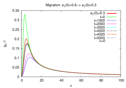
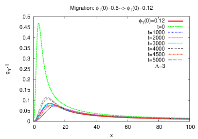
Migration of the strongly-perturbed U-oscillaton corresponding to , with a mass decrease of , towards a S-oscillaton. See also Fig. 18, where we show the evolved profile of the radial metric function of the -oscillaton migrating to the following S-branch configurations: for , for , for , and for .
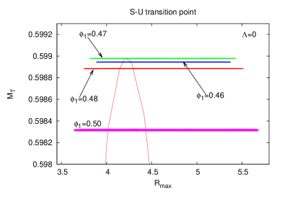
IV.3.6 The S-U transition point
We look carefully at the equilibrium configurations located nearby the critical configuration, .i.e., the most massive equilibrium configuration, see for instance Fig. 2, which is usually called the S-U transition pointAlcubierre et al. (2003). Fig. 19 shows the evolution of some slightly perturbed configuration near to the S-U transition point. With these examples we confirm previous results: S-oscillatons are intrinsically stable, whereas U-oscillatons are intrinsically unstable, no matter its proximity to the S-U transition point. Thus, this also confirms that the critical configuration is a true stability-instability transition point.
V Conclusions
In this work, we solved numerically the Einstein-Klein-Gordon system for a massive and real scalar field endowed with a scalar potential containing a quartic self-interaction term. The diverse numerical experiments confirm the same general properties found in the case of the free massive case, which are also present in the case of boson stars.
For all cases of the quartic self-interaction, it is found that there is a critical equilibrium configuration, which is the most massive one in each case; this critical configuration allows the separation of configurations into stable and unstable ones, the so-called S and U branches. As expected, the mass of the critical configuration increases for larger values of the quartic interaction.
Equilibrium configurations located on the S-branch are intrinsically stable, and vibrate with definite quasi-normal frequencies when slightly perturbed. If strongly perturbed, they can either migrate to another S-configuration, or collapse into a black hole, if its initial mass is smaller or larger, respectively, than the critical one. On the other hand, U-oscillatons are intrinsically unstable configurations. Under small perturbations, they are able to lose mass and migrate towards and equilibrium configuration on the S-branch, as long as its initial mass is not bigger than the critical one. However, under strong perturbations, U-oscillatons cannot prevent its collapse into black holes.
All in all, we have found that oscillatons with a quartic self-interaction share similar properties with their boson star counterparts. The larger the quartic interaction, the larger values the critical mass takes, but also the space for stable configurations is reduced because more diluted values of the scalar field are needed to sustain them. This can be seen in the shift of the critical scalar field value towards zero as the quartic interaction is increased.
It proved quite difficult to obtain equilibrium configurations for large values of the quartic interaction, because of the larger system of equations that must be solved in the case oscillatons (in terms of a Fourier expansion) as compared to the case of boson stars. Nonetheless, we have been able to explore the space parameter beyond the free case (), and provided evidence that points out to the close similarity of scalar configurations, whether we speak of real or complex scalar fields.
Acknowledgements.
SV-A thanks Carlos Palenzuela for useful comments, and acknowledges support from CONACyT, México, and the kind hospitality of the Canadian Institute for Theoretical Astrophysics (CITA), for a short research stay during which part of this work was done. RB acknowledges support from CONACyT, México under grants 83825. LAU-L thanks the Berkeley Center for Cosmological Physics (BCCP) for its kind hospitality, and the joint support of the Academia Mexicana de Ciencias and the United States-Mexico Foundation for Science for a summer research stay at BCCP. This work was partially supported by PROMEP, DAIP-UG, and by CONACyT México under grants 56946, and I0101/131/07 C-234/07 of the Instituto Avanzado de Cosmologia (IAC) collaboration.References
- Seidel and Suen (1991) E. Seidel and W. M. Suen, Phys. Rev. Lett., 66, 1659 (1991).
- Urena-Lopez et al. (2002) L. A. Urena-Lopez, T. Matos, and R. Becerril, Class. Quant. Grav., 19, 6259 (2002).
- Alcubierre et al. (2003) M. Alcubierre et al., Class. Quant. Grav., 20, 2883 (2003), arXiv:gr-qc/0301105 .
- Urena-Lopez (2002) L. A. Urena-Lopez, Class. Quant. Grav., 19, 2617 (2002), arXiv:gr-qc/0104093 .
- Balakrishna et al. (2008) J. Balakrishna, R. Bondarescu, G. Daues, and M. Bondarescu, Phys. Rev., D77, 024028 (2008), arXiv:0710.4131 [gr-qc] .
- Seidel and Suen (1994) E. Seidel and W.-M. Suen, Phys. Rev. Lett., 72, 2516 (1994), arXiv:gr-qc/9309015 .
- Balakrishna et al. (2006) J. Balakrishna, R. Bondarescu, G. Daues, F. Siddhartha Guzman, and E. Seidel, Class. Quant. Grav., 23, 2631 (2006), arXiv:gr-qc/0602078 .
- Colpi et al. (1986) M. Colpi, S. L. Shapiro, and I. Wasserman, Phys. Rev. Lett., 57, 2485 (1986).
- Guzman (2004) F. S. Guzman, Phys. Rev., D70, 044033 (2004), arXiv:gr-qc/0407054 .
- Grandclement et al. (2011) P. Grandclement, G. Fodor, and P. Forgacs, (2011), arXiv:1107.2791 [gr-qc] .
- Fodor et al. (2010) G. Fodor, P. Forgacs, and M. Mezei, Phys. Rev., D82, 044043 (2010a), arXiv:1007.0388 [gr-qc] .
- Fodor et al. (2010) G. Fodor, P. Forgacs, and M. Mezei, Phys. Rev., D81, 064029 (2010b), arXiv:0912.5351 [gr-qc] .
- Masso et al. (2005) E. Masso, F. Rota, and G. Zsembinszki, Phys. Rev., D72, 084007 (2005), arXiv:astro-ph/0501381 .
- Obregon et al. (2005) O. Obregon, L. A. Urena-Lopez, and F. E. Schunck, Phys. Rev., D72, 024004 (2005), arXiv:gr-qc/0404012 .
- Matos et al. (2008) T. Matos, J. A. Vazquez, and J. Magana, (2008), arXiv:0806.0683 [astro-ph] .
- Page (2004) D. N. Page, Phys. Rev., D70, 023002 (2004), arXiv:gr-qc/0310006 .
- Guzman and Rueda-Becerril (2009) F. S. Guzman and J. M. Rueda-Becerril, Phys. Rev., D80, 084023 (2009), arXiv:1009.1250 [astro-ph.HE] .
- Bernal and Siddhartha Guzman (2006) A. Bernal and F. Siddhartha Guzman, Phys. Rev., D74, 103002 (2006), arXiv:astro-ph/0610682 .
- Bernal and Guzman (2006) A. Bernal and F. S. Guzman, Phys. Rev., D74, 063504 (2006), arXiv:astro-ph/0608523 .
- Balakrishna et al. (1998) J. Balakrishna, E. Seidel, and W.-M. Suen, Phys. Rev., D58, 104004 (1998), arXiv:gr-qc/9712064 .
- Seidel and Suen (1990) E. Seidel and W.-M. Suen, Phys. Rev., D42, 384 (1990).
- Wiliam H. Press and others. (1992) S. A. T. Wiliam H. Press and others., Numerical Recipes in C: The Art of Scientific Computing, 2nd ed. (Press Syndicate of the University of Cambridge, 1992).