Role of Degeneracy, Hybridization, and Nesting
in the Properties of Multi-Orbital Systems

Abstract

To understand the role that degeneracy, hybridization, and nesting play in the magnetic and pairing properties of multiorbital Hubbard models we here study numerically two types of two-orbital models, both with hole-like and electron-like Fermi surfaces (FS’s) that are related by nesting vectors $(\pi,0)$ and $(0,\pi)$. In one case the bands that determine the FS’s arise from strongly hybridized degenerate d_xz and d_yz orbitals, while in the other the two bands are determined by non-degenerate and non-hybridized $s$-like orbitals. Using a variety of techniques, in the weak coupling regime it is shown that only the model with hybridized bands develops metallic magnetic order, while the other model exhibits an ordered excitonic orbital-transverse spin state that is insulating and does not have a local magnetization. However, both models display similar insulating magnetic stripe ordering in the strong coupling limit. These results indicate that nesting is a necessary but not sufficient condition for the development of ordered states with finite local magnetization in multiorbital Hubbard systems; the additional ingredient appears to be that the nested portions of the bands need to have the same orbital flavor. This condition can be achieved via strong hybridization of the orbitals in weak coupling or via the FS reconstruction induced by the Coulomb interactions in the strong coupling regime. This effect also impacts the pairing symmetry as demonstrated by the study of the dominant pairing channels for the two models.

I Introduction

Among the several aspects of the study of the iron-based superconductors that are still controversial and unsettled, johnston the following two questions have attracted considerable attention: (i) Does the magnetic order observed in the parent compoundsdai arise from the nesting properties of the non-interacting (or high temperature) Fermi surfacemazin ; kuroki or should a better description be based on the superexchange Heisenberg interactions between localized magnetic moments?si (ii) What is the pairing mechanism, to what extent is the pairing symmetry determined by nesting and, what is the actual symmetry and momentum dependence of the pairing operator? In particular, what is the role that the orbital degrees of freedom play in this context?

The origin of the magnetic state is being vigorously debated. One proposal, based on fermiology, is the excitonic mechanism in which electron-hole pairs are formed by one electron and one hole from different FS’s nested with nesting vector ${\bf Q}$. In this context some studies disregard the orbital structure of the bandsmazin ; chubu ; tesa ; phil while others stress the role played by their orbital composition.raghu ; Daghofer:2009p1970 ; graser ; moreo ; kemper ; rong ; our3 Another approach focuses on the order of the localized moments that develop in the presence of strong Coulomb interactionssi ; yildirim ; uhrig ; kruger and relies on ab initio resultsnakamura ; anisimov that suggest that the pnictides are moderately, rather than weakly, correlated, conclusion supported by photoemission measurements indicating mass enhancements due to electron correlations as large as 2-3.lu

The pairing mechanism in the pnictides is also controversial. Most of the pairing operators that have been proposed in the literature either ignore the multi-orbital characteristics of the problem or consider Cooper pairs that are made out of electrons located at the same orbital. A majority of these previous studies have been performed in the weak coupling limit. The original proposal of the $s_{\pm}$ pairing state dealt with the overall symmetry of the pairing operator but without distinguishing among the spatial vs. orbital contributions to its particular form.mazin ; kuroki Other authors schmalian have considered a spin-fluctuation-induced pairing interaction and also assumed that Cooper pairs are predominantly made of electrons in the same orbital. A Random-Phase Approximation (RPA) analysis graser concluded that the pairing is, again, intraorbital, both for the A_1g ($s$-wave) and B_1g ($d$-wave) symmetries. Among the authors that have used the conceptually different strong coupling approach, some have studied effective single orbital models si while others incorporated two orbitals, goswami but still only considering intra-orbital pairing operators. The same model was also studied under a mean-field approximation seo with the assumption that exchange takes place between spins on the same orbitals and, again, only intraorbital pairs were proposed.

Among the early first studies of multiband superconductors, Suhl et al.suhl considered two tight-binding bands, hypothetically identified with $s$ and $d$ orbitals, and the effect of weak electron-phonon interactions. Under these assumptions, it was reasonable to expect that the Cooper pairs would be formed by electrons belonging to the same band. However, the actual orbital composition of the pairs was not addressed. The interacting portion of the Hamiltonian was written in the band representation and this model was proposed by analogy with models used in the BCS theory, assuming that emission and absorption of a phonon could occur in four ways. These four processes corresponded to pair scattering within each of the two FS’s and pair hopping from one FS to the other. This last process would occur if the exchanged phonon has enough momentum to allow the Cooper pair to jump from a FS to the other, and it can occur even if the orbitals do not hybridize to form the bands.hotta In this case, the expected pairing operator is the traditional on-site $s$-wave state of the BCS theory, with a momentum independent gap. In principle, independent gaps may arise on the different FS’ssuhl unless the orbitals are hybridized by the symmetries of the Hamiltonian, in which case the gaps will have to be related to each other and obey the symmetries of the system.moreo

The previous discussion applies to superconductors driven by the electron-phonon interaction. However, it is believed that the most relevant interactions in the pnictides are the Coulomb repulsion and Hund magnetic exchange. These interactions are more easily expressed in real space and in the orbital representation. In fact, the effective form of the Coulomb interaction in the band representation is more complicated than the expression provided by Suhl et al.suhl for the electron-phonon interaction. In particular, it has been shown chubu that a pair hopping term, such as the one introduced by Suhl et al. occurs only if the orbitals get hybridized to form the bands. If the orbitals are $not$ hybridized this type of term is not present in the effective interaction Hamiltonian. In addition, when the bands are made of hybridized orbitals, as it is the case for the iron pnictides,boeri the actual orbital structure of the pairs needs to be considered since due to the Coulomb repulsion on-site pairing is not expected to occur, and the overall symmetry properties of the pairing operators may be a function of their spatial and orbital components. Daghofer:2009p1970 ; moreo

To understand the role that the orbitals play in the case of electrons with strongly hybridized bands that are interacting via the Coulomb repulsion, as believed to occur in the case of the pnictides in the context of the magnetic scenario for superconductivity, in this manuscript we present and discuss Lanczos numerical, Hartree mean-field, and RPA studies of two different two-orbital models, both displaying identical Fermi surfaces. One of them is the well-known and widely used two-orbital model for the pnictidesraghu ; Daghofer:2009p1970 ; moreo based on the two strongly hybridized degenerate d_xz and d_yz orbitals of iron, while the second is a two-band “toy- model” (dubbed the $s$-model) whose bands arise from two non-hybridized, non-degenerate, $s$-like orbitals that is introduced here for the first time. The latter model has a FS qualitatively similar to that of the pnictides. In both cases a hole (electron) FS is located at the $\Gamma/M$ ($X/Y$) points of the Brillouin zone (BZ). The hole and electron FS’s are connected by nesting vectors $(\pi,0)$ and $(0,\pi)$. The role that the nesting and the orbitals play in the magnetic and pairing properties of these models will be here investigated and discussed, both in the weak and strong coupling regimes.

Besides its conceptual relevance, the results presented here should also be framed in the context of recent bulk-sensitive laser angle-resolved photoemission (ARPES) experiments shimojima on BaFe₂(As_0.65P_0.35)₂ and Ba_0.6K_0.4Fe₂As₂. The main conclusion of Ref. shimojima, is the existence of orbital independent superconducting gaps that are not expected from spin fluctuations and nesting mechanisms, but are claimed to be better explained by magnetism-induced interorbital pairing and/or orbital fluctuations. This is argued based on the observation that the $3z^{2}−r^{2}$ orbital that forms one of the hole pockets at the BZ center, but that does not have a nested partner with the same orbital at the electron pockets, nevertheless appears to develop a superconducting gap. Another interesting experimental result that challenges the role of nesting in the physics of the pnictides is a careful measurement of the de Haas-van Alphen (dHvA) effect in BaFe₂P₂, the end member of the series BaFe₂(As_1-xP_x)₂, indicating that this non-magnetic and non-superconducting compound displays the best nesting of all the compounds in the series.arnold

The manuscript is organized as follows. In Section II the models are introduced. The magnetic properties are presented in Section III while the pairing properties are the subject of Section IV. Section V is devoted to the conclusions.

II Models

II.1 $d$-model

The reference model that will be considered here is the widely-used two-orbital model Daghofer:2009p1970 ; moreo ; raghu based on the d_xz ($x$) and d_yz ($y$) Fe orbitals of the pnictides. Since the two orbitals are degenerate, an important detail is that the direction along which each orbital is defined is actually arbitrary. Two directions have been used in the literature: $x,y$raghu ; Daghofer:2009p1970 ; moreo with the $x$ and $y$ axes along the directions that connect nearest-neighbor iron atoms, and $X,Y$kuroki ; dhlee with the $X$ and $Y$ axis rotated 45^o with respect to the $(x,y)$ set. In terms of the d_xz and d_yz orbitals the tight-binding dispersion of the two-orbital model is given bywan

$$\begin{split}\xi_{xy}({\bf k})=[-(t_{1}+t_{2})(\cos k_{x}+\cos k_{y})-\\ 4t_{3}\cos k_{x}\cos k_{y}-\mu]\tau_{0}\\ -(t_{1}-t_{2})(\cos k_{x}-\cos k_{y})\tau_{3}-\\ 4t_{4}\sin k_{x}\sin k_{y}\tau_{1},\end{split}$$ (1)

where $\tau_{i}$, with $i=1,2,3$, are the Pauli matrices and $\tau_{0}$ is the $2\times 2$ identity matrix. The $\tau_{i}$ matrices act in orbital space. Note that $\xi_{xy}({\bf k})$ must transform as the A_1g representation of D_4h; in this representation $\tau_{0}$ transforms as A_1g, $\tau_{1}$ as B_2g, and $\tau_{3}$ as B_1g. However, if the degenerate $d$-orbitals are expressed in terms of the $(X,Y)$ axes as $(d_{X},d_{Y})$, then the tight-binding dispersion becomes:dhlee

$$\begin{split}\xi_{XY}({\bf k})=[-(t_{1}+t_{2})(\cos k_{x}+\cos k_{y})-\\ 4t_{3}\cos k_{x}\cos k_{y}-\mu]\tau_{0}\\ -(t_{1}-t_{2})(\cos k_{x}-\cos k_{y})\tau_{1}-\\ 4t_{4}\sin k_{x}\sin k_{y}\tau_{3}.\end{split}$$ (2)

Notice that the $XY$ basis is chosen just for the orbitals while in real space the system of coordinates is still given by $(x,y)$. $\xi_{XY}({\bf k})$ also has to transform as A_1g which means that, when the orbitals are defined in the $(X,Y)$ basis, then $\tau_{1}$ transforms as B_1g, and $\tau_{3}$ as B_2g. It can be shown that since $\tau_{1}$ is the matrix that indicates inter-orbital electron hopping, this kind of hopping happens between nearest-neighbors [next-nearest-neighbors] in the $(X,Y)$ [($x,y$)] representation.

As previously discussed, if the values of the parameters are set to $t_{1}=-1$, $t_{2}=1.3$, $t_{3}=t_{4}=-0.85$ and $\mu=1.54$ then the Fermi surface (shown in Fig. 1 together with the band dispersion) for the tight-binding Hamiltonian is in qualitative agreement with band structure calculations for the pnictides raghu once folding to the reduced BZ is performed. Note that the system is half-filled (two electrons per Fe site on average) and, due to the orbital degeneracy, each orbital is half-filled as well, despite the fact that the bands are not equally filled.

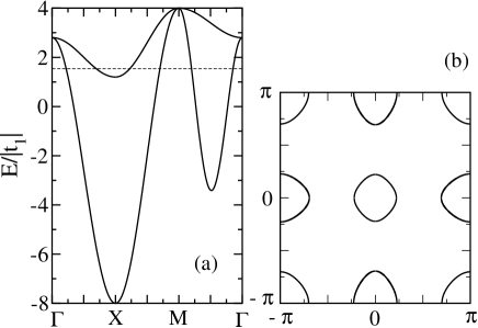
Figure 1: (a) Band dispersion and (b) Fermi surface for the half-filled two-orbital $d$-model for the pnictides, with the hopping parameters introduced in Ref. raghu, .

An important characteristic of the two degenerate $d$-orbitals in this model is that around the hole pockets a spinor describing the mixture of orbitals rotates twice on encircling these FS’s. The inversion and time reversal symmetry of the twice degenerate $d$ bands ensures that at each ${\bf k}$ point it is possible to choose real spinor wavefunctions that are confined to a plane. The spinor has vorticity $\pm 2$ around the hole pockets while there is no vorticity around the electron pockets.dhlee As pointed out in Ref. dhlee, , this topological characterization of the hole and electron pockets is also a characteristic of all the more realistic models for the pnictides that include additional orbitals.

II.2 $s$-model

Let us introduce now a two-orbital model with two non-degenerate non-hybridized $s$-like bands, called $s_{1}(1)$ and $s_{2}(2)$, with dispersion relations given by:

$$\xi_{s_{1}}({\bf k})=2t_{1}(\cos k_{x}+\cos k_{y})+4t_{2}\cos k_{x}\cos k_{y}-\mu,$$ (3)

and

$$\xi_{s_{2}}({\bf k})=2t_{3}(\cos k_{x}+\cos k_{y})+4t_{4}\cos k_{x}\cos k_{y}-\mu+\Delta,$$ (4)

where $\mu$ is the chemical potential and $\Delta$ is the energy difference between the two bands. The dispersions can also be written in the basis $(s_{1},s_{2})$, i.e., $(1,2)$, using the $\tau_{i}$ matrices as in the previous case:

$$\begin{split}\xi_{S}({\bf k})=[(t_{1}+t_{3})(\cos k_{x}+\cos k_{y})+\\ 2(t_{2}+t_{4})\cos k_{x}\cos k_{y}-\mu+{\Delta\over{2}}]\tau_{0}\\ +[(t_{1}-t_{3})(\cos k_{x}+\cos k_{y})+\\ 2(t_{2}-t_{4})\cos k_{x}\cos k_{y}-{\Delta\over{2}}]\tau_{3}.\end{split}$$ (5)

It is clear that here both $\tau_{0}$ and $\tau_{3}$ transform like A_1g and for this reason we call this model the $s$-model. In Fig. 2, the band dispersion (panel (a)) and the FS (panel (b), red circles) are shown for the parameter values $t_{1}=-0.05$, $t_{2}=0.7$, $t_{3}=-0.1$, $t_{4}=0.3$, $\Delta=2.8$ and $\mu=1.95$. The FS of the $d$-model is also shown (continuous black line) for comparison. They are obviously very similar, and precisely the goal of this effort is to investigate what kind of magnetic and pairing properties emerge from these two models that have nearly equal Fermi surfaces.

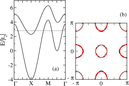
Figure 2: (color online) (a) Band dispersion and (b) Fermi surface of the half-filled two-orbital $s$-model given by Eq. (5) (red circles). The continuous line is the FS for the two-orbital $d$-model.

The hole pockets at the $\Gamma$ and $M$ points nest into the electron pockets at $X$ and $Y$, with nesting vectors $(0,\pi)$ and $(\pi,0)$. The system is half-filled but the individual bands/orbitals are not. Note that this is the case with the orbitals in the multi-orbital systems proposed for the pnictides, where nesting occurs between electron and hole pockets at the FS but none of the orbitals is exactly half-filled.graser ; kuroki

II.3 Coulomb Interaction

The Coulomb interaction term in both Hamiltonians is the usual one, with an on-site intraorbital (interorbital) Coulomb repulsion $U$ ($U^{\prime}$), and a Hund coupling $J$ satisfying the relation $U^{\prime}$=$U-2J$ for simplicity, and a pair-hopping term with coupling $J^{\prime}$=$J$. oles83 The full interaction term is given by

$$\begin{split}H_{int}=U\sum_{{\bf i},a}n_{{\bf i},a,\uparrow}n_{{\bf i},a,\downarrow}+{(U^{\prime}-J/2)\over{2}}\sum_{{\bf i},a}n_{{\bf i},a}n_{{\bf i},-a}\\ -J\sum_{{\bf i},a}{\bf S}_{\bf{i},a}\cdot{\bf S}_{\bf{i},-a}+{J\over{2}}\sum_{{\bf i},a}(d^{\dagger}_{{\bf i},a,\uparrow}d^{\dagger}_{{\bf i},a,\downarrow}d_{{\bf i},-a,\downarrow}d_{{\bf i},-a,\uparrow}+h.c.),\end{split}$$ (6)

where $d^{\dagger}_{{\bf i},a,\sigma}$ creates an electron with spin $\sigma$ at site ${\bf i}$ and orbital $a=x,y$ or 1, 2. ${\bf S}_{{\bf i},a}$ ($n_{{\bf i},a}$) is the spin (electronic density) of the orbital $a$ at site ${\bf i}$.

III Magnetic Properties

For a single-orbital model, the magnetic structure factor is easily defined as

$$S({\bf k})=\sum_{\bf r}e^{i{\bf k.r}}\omega({\bf r}),$$ (7)

with

$$\omega({\bf r})={1\over{N}}\sum_{\bf i}m({\bf i})m({\bf i+r}),$$ (8)

where $N$ is the number of sites of the lattice and

$$m({\bf i})=n_{{\bf i},\uparrow}-n_{{\bf i},\downarrow}=d^{\dagger}_{{\bf i},\uparrow}d_{{\bf i},\uparrow}-d^{\dagger}_{{\bf i},\downarrow}d_{{\bf i},\downarrow},$$ (9)

where $m({\bf i})$ denotes the net magnetization at site ${\bf i}$.

In a multiorbital system the net magnetization at site ${\bf i}$ is obtained in terms of the magnetization of each orbital $a$, and it is given by

$$m({\bf i})=\sum_{a}n_{{\bf i},a,\uparrow}-n_{{\bf i},a,\downarrow}=\sum_{a}(d^{\dagger}_{{\bf i},a,\uparrow}d_{{\bf i},a,\uparrow}-d^{\dagger}_{{\bf i},a,\downarrow}d_{{\bf i},a,\downarrow}).$$ (10)

While Eq. 10 characterizes the magnetization that is measured in experiments such as neutron scattering, it is natural to define generalized magnetic moments $m_{ab}({\bf i})$dhlee given by

$$m_{ab}({\bf i})=d^{\dagger}_{{\bf i},a,\uparrow}d_{{\bf i},b,\uparrow}-d^{\dagger}_{{\bf i},a,\downarrow}d_{{\bf i},b,\downarrow}.$$ (11)

With this definition, a generalized form of the magnetic correlation functions will depend on 4 orbital indices:

$$\omega_{abcd}({\bf r})={1\over{N}}\sum_{\bf i}m_{ab}({\bf i})m_{cd}({\bf i+r}).$$ (12)

Thus, it is possible to define orbital dependent magnetic structure factors given by:

$$S_{abcd}({\bf k})=\sum_{\bf r}e^{i{\bf k.r}}\omega_{abcd}({\bf r}).$$ (13)

These orbital-dependent operators may arise from processes as those depicted in panel (a) of Fig. 3, where having different orbitals at the two vertices is possible if the orbitals strongly hybridize to form a band.kemper

Figure 3: (a) Electronic process that gives rise to the orbital components of the structure factor. (b) Same as (a) but in the band representation.

The total orbital magnetic structure factor can then be defined as:

$$S_{TO}({\bf k})=\sum_{a,b,c,d}S_{abcd}({\bf k}).$$ (14)

Note that there are $M^{4}$ orbital dependent components of the generalized magnetic structure factor, where $M$ is the number of active orbitals in the system. The magnetization that is measured in neutron scattering experiments is given by Eq. 10, which in terms of the components of the tensor $m_{ab}$ becomes

$$m({\bf i})=\sum_{a}n_{{\bf i},a,\uparrow}-n_{{\bf i},a,\downarrow}=\sum_{a}m_{aa}({\bf i})=tr[m_{ab}({\bf i})].$$ (15)

Since $m({\bf i})$ is a trace its value is independent of the basis chosen to define the orbitals and it allows to calculate the experimentally measured local magnetization.

Notice that $m({\bf i})$ is the operator that has to be considered in order to construct the so-called homogeneous or diagonal structure factor defined in terms of the diagonal (intra-orbital) magnetic moments $m_{aa}({\bf i})$ and given by graser ; moreo

$$S_{MO}({\bf k})={1\over{N}}\sum_{a,b,{\bf r},{\bf i}}e^{i{\bf k.r}}m_{aa}({\bf i})m_{bb}({\bf i+r})=\sum_{a,b}S_{aabb}({\bf k}).$$ (16)

$S_{MO}$ is the physical magnetic structure factor that has to be calculated in the context of multiorbital systems to compare with neutron scattering results.Daghofer:2009p1970 ; moreo Several authors have pointed out the existence of the generalized components of the magnetic susceptibility both in the orbital representationgraser ; maria and in the band representation.phil It has also been pointed out that an orbital-transverse density-wave (OTDW) ordered state characterized by the non-homogeneous components of the magnetization tensor may develop in multi-orbital systems,yao an issue that will be further explored and discussed in the present work.

III.1 Non-interacting case

In order to understand the relationship between $S_{TO}$, $S_{MO}$, and the properties of the FS of the system, it is illuminating to consider the non-interacting case which can be easily studied in momentum space. Via a Fourier transform of $d^{\dagger}_{{\bf i},a,\sigma}$ and $d_{{\bf i},a,\sigma}$, $S_{abcd}$ in Eq. 13 can be written as

$$S_{abcd}({\bf k})=\sum_{{\bf p},{\bf q},\sigma,\sigma^{\prime}}(-1)^{\sigma+\sigma^{\prime}}d^{\dagger}_{{\bf q},a,\sigma}d_{{\bf q+k},b,\sigma}d^{\dagger}_{{\bf p},c,\sigma^{\prime}}d_{{\bf p-k},d,\sigma^{\prime}}.$$ (17)

In momentum space it is natural to use the band representation in which

$$\begin{split}S_{abcd}({\bf k})=\sum_{{\bf p},{\bf q},\sigma,\sigma^{\prime},\mu,\mu^{\prime},\nu,\nu^{\prime}}(-1)^{\sigma+\sigma^{\prime}}\\ <\mu|a>_{\bf q}<b|\mu^{\prime}>_{\bf q+k}<\nu|c>_{\bf p}<d|\nu^{\prime}>_{\bf p-k}\\ d^{\dagger}_{{\bf q},\mu,\sigma}d_{{\bf q+k},\mu^{\prime},\sigma}d^{\dagger}_{{\bf p},\nu,\sigma^{\prime}}d_{{\bf p-k},\nu^{\prime},\sigma^{\prime}},\end{split}$$ (18)

where $d^{\dagger}_{{\bf p},\nu,\sigma}$ creates an electron with momentum ${\bf p}$ and $z$-spin component $\sigma$ at band $\nu$, while $<\nu|a>_{\bf p}$ is the matrix element for the transformation from orbital to band representation.

In the band representation, the electronic processes that contribute to the magnetic correlations are shown in panel (b) of Fig. 3. Since the electronic band cannot change as the electron created at the right vertex is destroyed at the left vertex, in the band representation we can define band-dependent components of the structure factor given by

$$S_{\mu\nu\nu\mu}({\bf k})=\sum_{{\bf p},{\bf q},\sigma}d^{\dagger}_{{\bf q},\mu,\sigma}d_{{\bf q+k},\nu,\sigma}d^{\dagger}_{{\bf p},\nu,\sigma}d_{{\bf p-k},\mu,\sigma},$$ (19)

where the greek indices label the bands. A total structure factor can be defined in terms of $S_{\mu\nu\nu\mu}$ as

$$S_{TB}({\bf k})=\sum_{\mu,\nu}S_{\mu\nu\nu\mu}({\bf k}).$$ (20)

Also the homogeneous or diagonal magnetic structure factor $S_{MB}$, analogous of $S_{MO}$, can be defined as

$$S_{MB}({\bf k})=\sum_{\mu}S_{\mu\mu\mu\mu}({\bf k}),$$ (21)

since in the band representation $S_{\mu\mu\nu\nu}=0$, if $\mu\neq\nu$. Note that the band representation is the natural starting point in approaches based on fermiology.mazin ; chubu

In the noninteracting case being considered in this section, it is easy to show that

$$S_{\mu\nu\nu\mu}({\bf k})=2\sum_{\bf q}f_{\mu}({\bf q})[1-f_{\nu}({\bf q+k})],$$ (22)

where $f_{\mu}({\bf q})$ is the Fermi function for the band $\mu$. We also find that the components of the structure factor in the orbital representation are given by

$$\begin{split}S_{abcd}({\bf k})=2\sum_{{\bf q},\mu,\nu}<\mu|a>_{\bf q}<b|\nu>_{\bf q+k}\\ <\nu|c>_{\bf q+k}<d|\mu>_{\bf q}f_{\mu}({\bf q})[1-f_{\nu}({\bf q+k})].\end{split}$$ (23)

From the expressions in Eqs. 22 and 23 it can be shown that $S_{TO}=S_{TB}$ and $S_{MO}=S_{MB}$ only if the orbitals do not hybridize to form the bands, i.e., the matrix elements are the elements of the identity matrix. In case of a nonzero hybridization, then the structure factors in the band and orbital representations are different.

III.2 $d$-model

Numerical Lanczos calculations for the homogeneous (or diagonal) magnetic structure factor $S_{MO}$ have already been performed in previous literature for the two-orbital $d$-model indicating a tendency towards a magnetic stripe ordering for the undoped case, characterized by peaks at ${\bf k}=(\pi,0)$ and $(0,\pi)$ in $S_{MO}$.moreo This tendency is already apparent even in the non-interacting caseDaghofer:2009p1970 ; moreo as illustrated in panel (a) of Fig. 4 where $S_{MO}$ calculated in a $16\times 16$ cluster is shown with open circles, along the directions $(0,0)-(\pi,0)-(\pi,\pi)-(0,0)$ in the unfolded BZ. The broad peak at ${\bf k}=(\pi,0)$ is clear and it can be compared with the curve denoted by the star symbols in panel (b) of the same figure where results for the $\sqrt{8}\times\sqrt{8}$ cluster that can be studied numerically exactly (with the Lanczos algorithm and for any value of the Hubbard couplings) are presented. This same behavior is also apparent in the total orbital structure factor $S_{TO}({\bf k})$ indicated by the diamonds in Fig. 4(a).

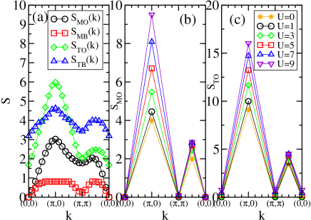
Figure 4: (color online) (a) Magnetic structure factors, total and homogeneous as indicated, for the non-interacting two-orbital $d$-model on a $16\times 16$ lattice. (b) Homogeneous orbital magnetic structure factor $S_{MO}({\bf k})$ for the interacting case with $J/U=0.25$ and at the indicated values of $U$. The results were obtained numerically using an 8-sites cluster and the Lanczos method. (c) Total orbital magnetic structure factor $S_{TO}({\bf k})$ for the interacting case, for the same parameters and technique as used in (b).

On the other hand, a calculation of the magnetic structure factor using the band representation, i.e. $S_{MB}({\bf k})$ indicated by the squares in panel (a) of Fig. 4, shows a rather different behavior: instead of a clear peak at $(\pi,0)$ there is a featureless plateau around $(\pi,0)$ that extends to $(\pi/2,\pi/2)$. This example demonstrates the importance of the matrix elements in Eq. 18 which differentiate between $S_{MO}$ and $S_{MB}$. In the non-interacting case, both functions can be expressed in terms of the Fermi functions as in Eqs. 22 and 23 allowing us to conclude that the peak at $(\pi,0)$ arises from the matrix elements rather than from purely nesting effects of the Fermi surfaces. Ignoring the matrix elements, it is interesting to note that a feature at $(\pi,0)$ can also develop if all the components of the structure factor in the band representation are considered and $S_{TB}({\bf k})$ is calculated, as shown by the curve indicated with triangles in Fig. 4(a).

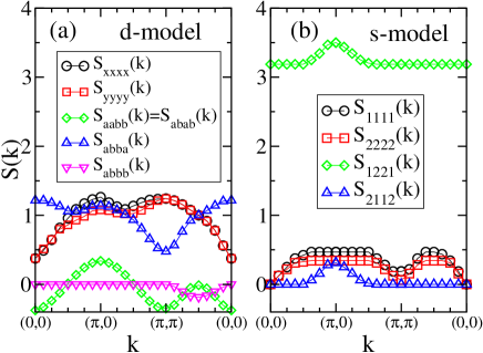
Figure 5: (color online) (a) Orbital-resolved components of the magnetic structure factor for the non-interacting two-orbital $d$-model on a $16\times 16$ lattice. (b) Band/orbital resolved components of the magnetic structure factor for the non-interacting two-orbital $s$-model also on a $16\times 16$ lattice. The index 1 (2) labels the lower (upper) band.

The contribution of the band- and orbital-resolved components of the structure factor in the non-interacting case are presented in panel (a) of Fig. 5. The components of the structure factor that contribute to $S_{MO}$ are $S_{aabb}$ with $a$ ($b$) taking the values $x$ ($y$) and $y$ ($x$) indicated by the diamonds in the figure, and $S_{aaaa}$ (indicated by the circles and squares). It is clear from the figure that the peak at $(\pi,0)$ in $S_{MO}$ at the non-interacting level is mostly due to the $S_{aabb}$ that arise from the nesting of the two bands that contain the same orbital flavors due to hybridization, while the components of the form $S_{aaaa}$ show features also at $(\pi,\pi)$ since this wave vector also nests the hole (electron) FS’s at $\Gamma$ and $M$ ($X$ and $Y$). It can be seen that the non-homogeneous components of the form $S_{abab}$ (diamonds) behave as $S_{aabb}$ in the non-interacting case and contribute to form the peak at $(\pi,0)$ in the total structure factor $S_{TO}$ [triangles in Fig. 4(a)]. For completeness in Fig. 5(a) orbital resolved structure factors of the form $S_{abba}$ (up triangles) and $S_{abbb}$ (down triangles) are also shown; $S_{abba}$ increase the value of $S_{TO}$ at $(\pi,0)$ while $S_{abbb}$ provide a small negative contribution to $S_{TO}$ along the diagonal direction of the BZ. Similar results were obtained for all the correlations in which three of the four indices are the same.

In non-interacting single-orbital systems, as studied for the cuprates, the spin and charge susceptibilities have the same form for all values of non-zero momenta, and any features in these functions arise from the nesting properties of the Fermi surface. Naively, the same is expected in the case of multi-orbital models but, as it will be discussed below, the hybridization of the orbitals plays a crucial role. In the $d$-model, the peaks in $S_{MO}$ appear to be associated with the nesting of the hole- and electron-like Fermi surfaces. In the weak coupling picture, it is expected that magnetic order with ${\bf Q}$ equal to the nesting moments stabilizes when repulsive Coulomb interactions are added. Our Lanczos calculations for $S_{MO}$ and $S_{TO}$, in panels (b) and (c) of Fig. 4, show that this is indeed the case.

The Lanczos calculated orbital magnetic structure factor $S_{MO}({\bf k})$, using a $\sqrt{8}\times\sqrt{8}$ sites cluster, is shown in Fig. 4(b) for different values of $U$ and at $J/U=0.25$. This structure factor has a peak at ${\bf k}=(\pi,0)$ (and $(0,\pi)$ as well, not shown) that becomes sharper as $U$ increases, indicating a tendency towards robust magnetic order. Mean-field calculations based on these results, but extended to much larger systems, indicate that actual magnetic order develops at a finite value of $U$.moreo ; rong

The Lanczos-evaluated behavior of the $S_{MO}({\bf k})$ peak at ${\bf k}=(\pi,0)$, as a function of $U$, is shown in Fig. 6(a), for two different values of $J/U$ (0.05 and 0.25). The tendency towards a robust magnetic state with increasing $U$ and $J/U$ is again clear.

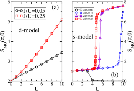
Figure 6: (color online) Orbital magnetic structure factor at wave vector $(\pi,0)$ calculated numerically (Lanczos). (a) Results for the two-orbital $d$-model, as a function of the Coulomb repulsion $U$ and for the values of $J/U$ indicated. (b) Same as (a) but for the $s$-model.

As previously stated, $S_{MO}$ is the magnetic structure factor calculated in the literature for comparison with experiments, but for completeness and for the sake of comparison with the $s$-model results, in panel (c) of Fig. 4, we present the Lanczos calculated values for the total generalized magnetic moment $S_{TO}$ for the $d$-model as a function of $U$, for the case $J/U=0.25$. It is clear that for the $d$-model $S_{TO}$ mimics the behavior of $S_{MO}$. An important question to ask is what are the components of the orbital-resolved magnetic structure factor that drive the development of a peak at ${\bf Q}=(\pi,0)$ (and $(0,\pi)$) when the Coulomb interactions are active. In Fig. 7 partial sums over selected components of the structure factor are shown with summations performed over repeated indices. In panel (a) of Fig. 7 it can be clearly observed that $S_{aabb}$, whose sum over $a$ and $b$ are indicated by the plus signs and the continuous lines in different shades for the different values of the interaction, are the components that drive that magnetic behavior. In fact, these are the homogeneous components that contribute to the physical magnetic structure factor $S_{MO}$. It is interesting to note that while $\sum_{a,b}S_{aabb}$ is equal to $\sum_{a,b}S_{abab}$ in the non-interacting system (panel (a) of Fig. 5) the partial sum of the non-homogeneous component $\sum_{a,b}S_{abab}$ [x symbols and dotted lines in Fig. 7(a)] does not increase with $U$ at ${\bf Q}$ while the partial sum $\sum_{a,b}S_{aabb}$ clearly does.

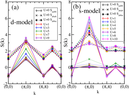
Figure 7: (color online) Orbital-resolved components of the total structure factor (sums over repeated indices are implied): $S_{aabb}$ (plus, full line), $S_{abab}$ (x, dotted line) and $S_{abba}$ (star, dashed line), for the values of $U$ indicated, obtained numerically (Lanczos) at $J/U=0.25$ using an 8-sites cluster for (a) the $d$-model and (b) the $s$-model.

III.3 $s$-model

Let us now carry out a similar analysis but for the two-orbital $s$-model defined by Eq. 5. Since in this model each band is defined by a single orbital, then it is clear that $S_{MO}=S_{MB}$ and $S_{TO}=S_{TB}$.foot Note that studies based on fermiology assume that if hole and electron FS’s are nested via a momentum vector ${\bf Q}$, then spin density wave order will arise from a logarithmic instability that develops in the spin response at ${\bf Q}$ and is stabilized by the Coulomb interaction.mazin ; chubu In this scenario the spin-density wave originates from the formation of particle-hole pairs, excitons, belonging to the electron and hole FS’s (excitonic mechanism).chubu Our goal is to investigate whether this mechanism is valid for the $s$-model.

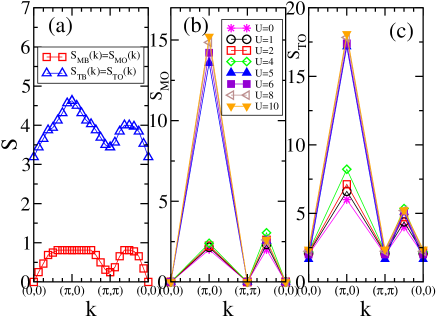
Figure 8: (color online) (a) Magnetic structure factors (total and homogeneous) as indicated for the non-interacting two-orbital $s$-model using a $16\times 16$ lattice. (b) Homogeneous orbital/band magnetic structure factor $S_{MO}({\bf k})$ for the interacting case with $J/U=0.25$, at the indicated values of $U$. The results were obtained numerically via the Lanczos method using an 8-sites cluster. (c) Total orbital/band magnetic structure factor $S_{TO}({\bf k})$ for the interacting case with the same parameters as in (b).

The magnetic structure factor $S_{MO}$ in the non-interacting limit, denoted by the squares in panel (a) of Fig. 8, does not show the features expected from the nesting of the two Fermi surfaces at momentum ${\bf Q}$. The structure factor is actually rather flat on all the BZ, vanishing at ${\bf k}=(0,0)$ and $(\pi,\pi)$. These results are not what it would have been expected from the nesting properties.

Note that the results for $S_{MO}$ in the non-interacting $s$-model [squares in Fig. 8(a)] are actually identical to the results for the homogeneous structure factor in the $d$-model in the band representation $S_{MB}$ [indicated by squares in Fig. 4(a)], since both systems do have the same FS. However, note how different are the results for the $d$-model in the orbital representation [indicated by circles in Fig. 4(a)]. This is due to the effect of the matrix elements that result from the hybridization of the orbitals, which play a crucial role in the magnetic properties of the system. This effect can be more clearly appreciated when the interactions are added. The behavior of the peak in $S_{MO}({\bf k})$ at ${\bf k}=(\pi,0)$ was calculated with the Lanczos method applied to the $s$-model, by varying $U$ and at different values of $J/U$ using an $N=8$ sites tilted cluster. In Fig. 6(b) it can be observed that for values of $J<0.1U$ the peak in $S_{MO}$ eventually vanishes. On the other hand, for $J\geq 0.1U$ a rapid increase in the peak’s magnitude suddenly occurs at a value of $U$ that decreases as $J/U$ increases. The increase of the peak at $(\pi,0)$ with increasing $U$ is contrasted with the behavior of the feature at $(\pi/2,\pi/2)$ displayed in Fig. 8(b). Examination of the numerical (Lanczos) ground state indicates that at this point the Hubbard interaction is strong enough to hybridize the two bands and develop magnetic stripe order.

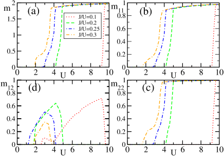
Figure 9: (color online) Mean-field calculated orbital/band resolved magnetic order parameters for the $s$-model, as a function of $U$ and for the indicated values of $J/U$. (a) Total homogeneous magnetic order parameter $m=m_{11}+m_{22}$; (b) $m_{11}$; (c) $m_{22}$; (d) $m_{12}=m_{21}$.

Based on the numerical results discussed above a Hartree-Fock mean-field calculation was performed, following technical aspects already widely discussed in previous literature.rong By this procedure we found that the total (homogeneous) magnetization $m$ shown in panel (a) of Fig. 9 mimics the behavior of $S_{MO}(\pi,0)$. Here, the transition to the magnetically ordered state is very rapid, resembling a first-order transition. We observed that MF magnetic order develops only if $J\geq 0.1U$ which is in agreement with the Lanczos results shown in Fig. 6(b). The mean-field results also indicate that a full gap characterizes the magnetic state which is then an insulator as it can be seen from the MF calculated spectral functions $A({\bf k},\omega)$ displayed on panel (a) of Fig. 10. It is clear that the hybridization of the original bands/orbitals due to the Coulomb interaction is very strong and the band structure has been totally reconstructed. This behavior can be understood in the real-space representation. In order to develop magnetic stripes in the half-filled system, it is necessary to have a net magnetic moment on each site. In the $d$-model, each orbital is half filled and thus contains a spin-$1/2$ that can easily be polarized by the interaction. In the $s$-model, on the other hand, the orbitals correspond to the bands, and one orbital is thus almost filled while the other is almost empty. Then, there are far fewer magnetic moments that can be polarized.

Thus, we observe that in the $s$-model the peak at ${\bf Q}$ in the magnetic structure factor does not develop from the nesting of the FS but from the Coulomb interaction, and it occurs fairly suddenly and at a robust value of $U\geq 4$ for the hopping parameters used here. Thus, while nesting appears to be a needed condition for the development of the peak in the magnetic structure factor, it is not a sufficient condition. The hybridization of the orbitals needs to be present such that the matrix elements allow the peak to emerge at sufficiently strong coupling. In fact, it is necessary that the bands that are connected by the nesting vector ${\bf Q}$ share the same orbital flavor. If this occurs via hybridization, magnetic order can develop at relatively weak coupling, but if this is not the case, the Coulomb interaction would induce magnetic order only in the strong coupling regime, as we have verified by studying the $s$-model. In this case, the magnetic transition is also a metal-insulator transition, as observed at least within the mean-field approximation. The $d$-orbital model, on the other hand, is known to display an intermediate metallic magnetic phase.rong Thus, the present results indicate that the $s$ and $d$ models develop similar magnetic behavior only in the strong coupling regime while in weak coupling, despite the nearly identical Fermi surfaces, both models have quite different ground states.

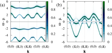
Figure 10: (color online) Intensity of the mean-field calculated spectral functions $A({\bf k},\omega)$ as a function of $\omega-\mu$ and ${\bf k}$ for the $s$-model: (a) in the stripe magnetic phase for $U=5$ and $J/U=0.25$; (b) in the phase with orbital-transverse spin order for $U=2.5$ and $J/U$=0.25.

III.3.1 Orbital-transverse spin order

While the analysis of the results for the $s$-model presented above indicates that, despite the nesting of the electron and hole FS’s, no magnetic order, as defined by the homogeneous operator, develops in weak coupling, it is instructive to analyze the behavior of the non-homogeneous components and the total magnetic structure factor $S_{TO}$. The non-interacting values of $S_{TO}$ on a $16\times 16$ lattice are indicated by the triangles in panel (a) of Fig. 8. There is a feature at $(\pi,0)$ arising from the contribution of the interband components of the form $S_{abba}\equiv S_{\mu\nu\nu\mu}$, shown by the triangles and diamonds in panel (b) of Fig. 5. These are the components of $S_{abcd}$ that contribute to the development of the maximum at ${\bf Q}=(\pi,0)$ (and $(0,\pi)$) because the nesting at ${\bf Q}$ is between FS’s defined by different bands. However, this type of terms are not part of the definition of the homogeneous structure factor $S_{MB}$. On the other hand, the components of the form $S_{aaaa}$ indicated with circles and squares in Fig. 5(b), have a very flat shape in all the BZ and do not produce a sharp feature. Any other combination of orbital indices does not contribute to $S_{TO}$ as shown in Eq. 22.

The effect of the Coulomb interactions on the feature at $(\pi,0)$ in $S_{TO}$ has been obtained with Lanczos calculations and it can be seen in panel (c) of Fig. 8. The peak slowly increases as $U$ raises from 0 to 4. Notice that for the same range of values of $U$ the peak in $S_{MO}$ shown in panel (b) of the figure does not change. The obvious question is whether this behavior indicates a novel kind of order in multi-orbital systems. The answer is provided via our MF approach that allows us to evaluate the components of the magnetization $m_{ab}$. The homogeneous magnetization $m$ displayed in panel (a) of Fig. 9 is obtained as the sum of the intraorbital magnetizations $m_{11}$ and $m_{22}$ shown in panels (b) and (c) of the figure. Interestingly, we found that the non-diagonal components $m_{12}=m_{21}$ develop finite values while the diagonal components are zero for values of $J/U>0.1$ as shown in panel (d) of the figure. At the MF level we can study the real space configuration associated to this finite order parameter. We have observed that the orbital spins are disordered, which is expected by the lack of features in $S_{MO}({\bf k})$, but there are ordered generalized spins ${\bf G}_{ab}({\bf i})$ defined as

$${\bf G}_{ab}({\bf i})=d^{\dagger}_{{\bf i},a,\alpha}\vec{\sigma}_{\alpha,\beta}d_{{\bf i},b,\beta},$$ (24)

where $\vec{\sigma}$ are the Pauli matrices and the orbital indices $a\neq b$. In Fig. 11 we show two configurations of ${\bf G}_{12}({\bf i})$ that provide the MF ground state associated with the peak in $S_{TO}$ at $(\pi,0)$ (and $(0,\pi)$) when $m_{12}$ is finite. Panel (a) shows a flux configuration that generates peaks at $(\pi,0)$ and $(0,\pi)$ in $S_{TO}$ and panel (b) shows a stripe configuration that produces a peak at $(0,\pi)$. The peak at $(\pi,0)$ is generated by a companion configuration rotated by $\pi/2$. Flux and stripe configurations have energies very close to each other and the actual ground state depends on the parameters.eremin

Figure 11: Schematic representation of the real space mean-field calculated ground states for the $s$-model when $m_{12}$ is non-zero. (a) Flux phase; (b) Stripe phase. The dots indicate the sites and the arrows represent the MF value of the generalized spin ${\bf G}_{12}({\bf i})$ defined in the text.

The new phase hinted at by the Lanczos calculations and stabilized in the MF calculations is insulating. The MF calculated spectral functions are shown in panel (b) of Fig. 10. A full gap has developed at the FS indicating that this order, if realized, would be observed with ARPES measurements. On the other hand, neutron scattering experiments would not detect it. This can be seen by performing a rotation in orbital space given byyao

$$d^{\dagger}_{{\bf i},\pm,\sigma}={1\over{\sqrt{2}}}(d^{\dagger}_{{\bf i},1,\sigma}\pm d^{\dagger}_{{\bf i},2,\sigma}).$$ (25)

In this new basis the schematic representations of the spins are shown in Fig. 12. It is clear that while the homogeneous spins in the orbitals + (black dots) and - (white dots) are ordered, the net spin at each site is 0 and thus, neutron scattering experiments will not detect the order because there is no finite local magnetization. These phases appear to be a realization of the orbital-transverse density-wave (OTDW) order proposed in Ref. yao, .

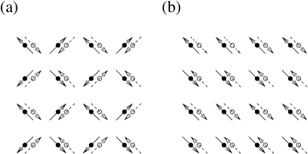
Figure 12: Schematic representation of the real space mean-field calculated ground states for the $s$-model when $m_{12}$ is non-zero: (a) Flux phase; (b) Magnetic stripe phase. The black and white dots represent the orbitals + and - at each site and the continuous and dashed arrows represent the MF value of the spin at each orbital.

Summarizing, a careful analysis of the small-cluster ground states obtained via Lanczos techniques, and with mean-field approximations in larger clusters, highlights the important role that the orbital composition plays in the development of magnetic order.

For the $s$-model, it is illuminating to consider the behavior of the total magnetic structure factor $S_{TO}$, see panel (c) of Fig. 8, calculated numerically as the interactions are increased. There is a weak increase of $S_{TO}$ at ${\bf Q}$ before the sudden jump at $U=4$. The behavior of the resolved components displayed in panel (b) of Fig. 7 shows that for $0\leq U\leq 4$ the partial sum over $a$ and $b$ of the non-homogeneous components $S_{abab}$ (x symbols and dotted line) and $S_{abba}$ (star symbols and dashed lines) increases in value at $(\pi,0)$ indicating the stabilization of the orbital-transverse spin phase. For $U>4$ a sudden increase of the sum of the homogeneous components $S_{aabb}$ (plus symbols and continuous line) develops, the non-homogeneous components start to decrease and homogeneous magnetic order is established.

III.4 Weak Coupling: RPA Analysis

Additional insight into the weak coupling behavior of the $d$- and $s$-models can be obtained via the diagrammatic RPA method. Using this technique, the magnetic susceptibility $\chi_{abcd}({\bf k},i\omega)$ was calculated, graser ; kemper and the static structure factor was obtained by integrating the results over $\omega$.ogata In panel (a) of Fig. 13, the RPA-calculated diagonal or homogeneous structure factor for the $d$-model is presented. The non-interacting result (in agreement with the results indicated by the circles in panel (a) of Fig. 4) are denoted by the dashed line, while results at $U=2.64$, the coupling strength where divergent behavior is about to occur for the case $J/U$=$0.25$, are indicated by the continuous line. In these results the peak at $(\pi,0)$ is very prominent both with and without the Hubbard interaction on.

The same calculation performed for the $s$-model, presented in panel (b) of Fig. 13, gives rather different results. The flat behavior in the noninteracting case (dashed line), in agreement with the curve indicated by squares in Fig. 8(a), is replaced within RPA by a curve (continuous line) that develops weak features at incommensurate values of the momentum. Note that there were no precursors of these features in the non-interacting limit. Eventually the peak the closest to the $\Gamma$ point along the diagonal direction of the BZ, indicated with an arrow in the figure, was found to diverge when $U$ becomes larger than 2.67 for $J/U=0.25$. This appears to be an illustration of a case in which RPA calculations indicate magnetic behavior that is unrelated to nesting properties. The RPA results show that an excitonic weak-coupling picture in which magnetic order characterized by the nesting momentum ${\bf Q}$ is expected to occur can be misleading if the orbital composition of the bands is not incorporated into the discussion. In the excitonic picture, the expectation is that the Coulomb interaction will allow the formation of electron-hole pairs with the electron (hole) in the electron (hole) Fermi surface. Since $S_{MO}$ incorporates intraorbital electron-hole pairs, an RPA response requires that the nesting vector connects parts of the electron and hole bands that contain the same orbital flavor. This is the case in the $d$-model where even in the weak coupling regime the $(\pi,0)$ magnetic-stripe state with two electrons with parallel spins at every site of the lattice has the largest weight in the ground state according to our Lanczos numerical studies. Since both orbitals are degenerate, the energetic penalization for populating both orbitals is $U^{\prime}$ and there is a gain given by $J$ if both spins are parallel. As discussed before, in the $s$-model, on the other hand, the orbitals are non-degenerate and, thus, in addition to $U^{\prime}$ there is an energy $\Delta$ of penalization when two electrons are located in different orbitals at the same site. This energy can be larger than the gain obtained from $J$ by having parallel spins or than the $U$ penalization that arises from introducing both electrons in the same orbital. Then, a magnetic “stripe” state can only develop when $U$ is comparable to the splitting $\Delta$. This regime, which develops in strong coupling according to our Lanczos and MF calculations, is not captured by the weak-coupling RPA method. However, it will be shown that RPA is effective at finding the orbital-transverse spin state presented in the previous section if the generalized structure factor $S_{TO}$ is calculated.

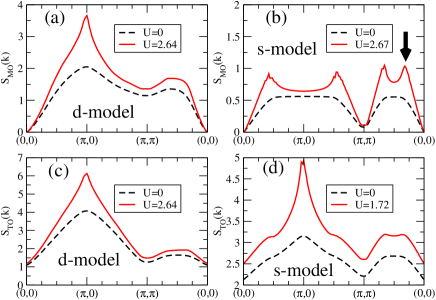
Figure 13: (color online) RPA calculated magnetic structure factors for $J/U=0.25$, at the values of $U$ indicated (full line). The non-interacting results are indicated with dashed lines. (a) Homogeneous magnetic structure factor in the $d$-model. (b) Same as (a), but for the $s$-model. The arrow indicates the peak that grows the most as the critical $U$ is reached. (c) Generalized magnetic structure factor for the $d$-model. (d) Same as (c), but for the $s$-model.

The values of $S_{TO}$ obtained with RPA are presented in panels (c) and (d) of Fig. 13 for the $d$ and $s$ models, respectively. Both develop a peak at the nesting wavevector. The generalized structure factor takes into account electron-hole pairs formed by an electron and a hole in different bands that are allowed to have different orbital flavors. This is the reason why a peak develops now in both cases. While in the case of the $d$-model the behavior of $S_{TO}$ mimics $S_{MO}$ and the divergence in both occurs at the same value of $U$ (slightly above 2.64 for $J/U=0.25$) indicating that the stripe-magnetic order is the cause, in the $s$-model the peak in $S_{TO}$ develops at a lower value of $U$ ($U=1.72$ for $J/U=0.25$) and it results from the ordering revealed by the inhomogeneous components $S_{1221}$ and $S_{2112}$ of the structure factor, i.e., orbital-transverse spin order as discussed in the previous section. In this new light, we see that the divergence in $S_{MO}$ should be disregarded since it occurs for a much larger value of $U$ than the divergence in $S_{TO}$. These results show that if all the elements of the susceptibility tensor are considered, RPA calculations are able to determine the development of new ordered phases that can develop in multi-orbital systems. Conversely, in multi-orbital systems in which orbital-transverse order develop, RPA calculations using only the homogeneous susceptibility may lead to unphysical results.

III.5 Strong Coupling Regime

In the regime where the coupling $U$ is sufficiently strong such that even in the $s$-model it is energetically favorable to locate two electrons with parallel spins at the same site (and in different orbitals), both the $s$- and $d$-models can be mapped into effective $t-J-J^{\prime}$ models and an insulating state with magnetic stripes can occur. In this case the Hubbard repulsion has effectively hybridized both bands causing large distortions and actually opening a full gap [see Fig. 10(a)]. In this strong coupling regime both models appear to have similar properties, but an insulating magnetic behavior does not reproduce the experimental behavior observed in several of the undoped iron pnictides (such as the 1111 and 122 families). However, this regime could be applied to the chalcogenides: if $U$ is sufficiently strong the magnetic behavior that develops in the strong coupling limit is more related to the hopping parameters and superexchange than to the weak-coupling nesting properties of the Fermi surface. While the values of the hopping parameters in the Hamiltonian are crucial to achieve nesting in weak coupling,maria systems in which nesting is not perfect can develop stripe-like magnetic order if they map into a $t-J-J^{\prime}$si model in the strong coupling limit such as in the case of the three-orbital model for the pnictides.our3

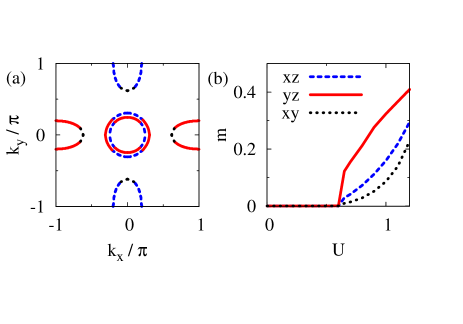
Figure 14: (color online) (a) Fermi surface with its orbital composition for the case of a three-orbital model for the pnictides. (b) Mean-field calculated orbital-resolved magnetization for the same three-orbital model. The figure was taken from Ref. our3, for illustration.

The results in this section indicate that in the case of the pnictides, even if the five $d$ orbitals are considered, the $xz$ and $yz$ orbitals are the most likely to produce the strongest contribution to the metallic stripe magnetic order at weak or intermediate values of the Hubbard interaction because they are the major constituents of the FS’s with better nesting and because they are degenerate and, thus, there is no energy $\Delta$ that needs to be overcome by the interaction. This is apparent already in the three-orbital model for the pnictides, where a mean-field calculation shows that magnetic order develops at a finite value of $U$ (see panel (b) of Fig. 14).our3 In Fig. 14(a) it can be observed that the orbital with the best nesting associated with ${\bf Q}=(\pi,0)$ is the $yz$ one, indicated by the continuous line. A mean-field calculation of the orbital resolved magnetization $m_{aa}$ for $a$=$xz$, $yz$, and $xy$, shows that $m_{yz,yz}$ grows very rapidly at the lowest value of $U$. The magnetizations for the other orbitals develop as $U$ hybridizes and distorts the original bands. Thus, in the intermediate $U$ regime when magnetism develops, the $xz$ and $yz$ orbitals are the ones that would develop the stronger magnetization (albeit for different values of ${\bf Q}$) giving rise to a magnetic metallic phase. Thus, nesting seems to drive the magnetization of the $xz/yz$ orbitals while the additional orbital hybridizations that develop due to the reconstruction of the FS then drives the smaller magnetization in the remaining orbitals.

IV Pairing Symmetries

Regarding the symmetry of the pairing operators corresponding to the models analyzed here, previous numerical calculations have indicated a competition between A_1g, B_2g, and E_g states in the $d$-model,moreo ; nicholson as shown in panel (a) of Fig. 15. The E_g states correspond to a $p$-wave spin-triplet state that becomes destabilized upon the addition of binding-enhancing Heisenberg terms.nicholson The favored pairing operators with the symmetry A_1g are all trivial in their orbital composition, i.e. they are intra-orbital with the form $D^{\dagger}\sigma_{0}D$ where $D^{\dagger}=(d^{\dagger}_{{\bf k},x,\uparrow},d^{\dagger}_{-{\bf k},y,\downarrow})$ in the $({x,y})$ basis, and they remain intraorbital in the $({X,Y})$ basis. However, the B_2g pairing operators have a non-trivial orbital composition given by $D^{\dagger}\sigma_{1}D$ in the basis $({x,y})$, indicating that the pairs are made of electrons in the two different orbitals. In the $({X,Y})$ basis the B_2g pairing operator becomes $D^{\prime\dagger}\sigma_{3}D^{\prime}$ with $D^{\prime\dagger}=(d^{\dagger}_{{\bf k},X,\uparrow},d^{\dagger}_{-{\bf k},Y,\downarrow})$. Thus, in the $(X,Y)$ representation the B_2g pairs are intraorbital but there is an important sign difference between the pairs in the different orbitals which makes the orbital contribution intraorbital but non trivial. It is interesting to observe that the intraorbital B_1g state found with RPA calculations in the five-orbital model for the pnictides graser would become interorbital in the $(X,Y)$ basis.

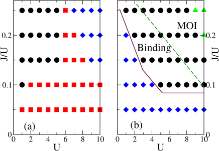
Figure 15: (color online) (a) Relative symmetry between the undoped and the electron-doped ground states for the case of the $d$-orbital model, varying $J/U$ and $U$. The results were obtained numerically via the Lanczos method using a small cluster with $N=8$ sites (and following steps already discussed in previous literature).Daghofer:2009p1970 ; nicholson The circles indicate states with $E_{g}$ symmetry, squares correspond to $B_{2g}$, and diamonds represent $A_{1g}$ symmetric states. (b) Same as (a) but for the $s$-model with the triangles denoting B_1g symmetry. In the region above the continuous line the two added electrons form a bound state. The dashed line indicates the boundary for the stability of the magnetically ordered insulating (MOI) region in the undoped state.

The results for the $s$-model regarding pairing properties are different from those in the $d$-model. Following previous investigations,Daghofer:2009p1970 using the Lanczos method we have calculated the relative symmetry between the undoped (number of electrons $N_{e}=16$) and electron-doped ($N_{e}=18$) states, as an indicator of the possible pairing symmetry in the bulk limit. The results are presented in panel (b) of Fig. 15, varying $U$ and $J/U$. For small values of $U$ and $J/U$ the doped ground state has symmetry $A_{1g}$ in agreement with the $d$-model, although in a different regime of couplings. Increasing $U$ and $J/U$, the $s$-model ground state switches to the $E_{g}$ symmetry, i.e. $p$-wave. This $p$-symmetry arises from the spatial location of the electrons since the orbital contribution is trivial. We have observed that in the small cluster studied here the spin-triplet state with ${\bf k}=(0,0)$ is almost degenerate with a spin-singlet state with ${\bf k}=(\pi,\pi)$. The possibility of having a spin-singlet $p$-wave state with wavevector ${\bf k}=(\pi,\pi)$ has been previously discussed long ago in the context of the single-orbital Hubbard model.scz In the present case, we need to remember that here ${\bf k}$ is a pseudo-momentum and in the folded representation ${\bf k}=(\pi,\pi)$ actually maps into $(0,0)$ so that the actual Cooper pair, if stabilized, has zero center-of-mass momentum, but the components of the pair belong to bonding and antibonding bands that could become hybridized for the large values of the interactions needed to stabilized these states. As indicated in the figure, it was also found that the $p$-states show binding in the small system studied here. In addition a small region of bound states with B_1g symmetry is found at even larger couplings. While in the $d$-model our numerical results indicate that the orbital degree of freedom plays a crucial role in the symmetry of the pairing states, we observe that this is not the case in the $s$-model. This result seems to indicate that interorbital Cooper pairs are likely to be present in multi-orbital systems with strongly hybridized bands as it is the case of the pnictides.

Understanding more deeply why the $s$-model develops its particular pairing properties is at this point unnecessary since the model simply provides an illustration of a system with a similar FS as the $d$-model, and the goal of this work was to show that the orbital composition of the bands plays a crucial role in determining the symmetry of the doped states. The examples that have been discussed here clearly show that models with the same Fermi surface and the same interactions can have very different pairing properties depending on the degree of hybridization of the orbitals. It also seems, according to the present results, that the relevance of the orbital degree of freedom in determining the pairing symmetry is also influenced by the degree of hybridization among those orbitals.

V Conclusions

Summarizing, numerical and analytical calculations have been performed in order to compare the properties of two band models with identical FS’s and interactions, but differing in the degree of hybridization of the orbitals to form the bands. Despite the nesting properties of the FS’s it was discovered that both models have similar magnetic (insulating) ground states in the strong coupling limit, but they are very different in weak and intermediate coupling. The $s$-model offers an example in which despite the nesting of the FS and the presence of Coulomb interactions, magnetism does not develop in weak coupling. However, it was discovered that instead, as a result of the nesting in weak coupling, the Coulomb interaction stabilizes an orbital-transverse spin ordered state with no local magnetization. This state is insulating and is characterized by a gap that could be observed in ARPES experiments. However, due to the lack of local magnetization, neutron scattering experiments would not detect the development of “generalized spin order”. In fact, standard RPA calculations in the $s$-model lead to incorrect results such as incommensurate magnetic order in the physical homogeneous channel. However, when the non-homogeneous components of the susceptibility are taken into account, RPA reveals the existence of the orbital-transverse spin phase for values of $U$ lower than the ones needed to observe the unphysical magnetic state.

It is clear that the physical (homogeneous) magnetic structure factor depends strongly on the orbital flavor of the bands and for this quantity to develop a peak in weak coupling it is necessary that the portions of the FS connected by nesting have the same orbital flavor.

The possibility of “hidden” magnetic ordering in the pnictides has been proposed by several authorsrodriguez ; cricchio ; bascones as an explanation for the unexpectedly low value of the magnetization in several of these materials. The hidden order proposed by these authors was “diagonal”, as the configurations we presented in Fig. 12 after transforming our non-diagonal results into a rotated orbital basis. However, in multi-orbital systems with more than two orbitals, it may be necessary to consider the non-diagonal order as well. In theoretical and analytical calculations these non-diagonal hidden orders are revealed by considering all the components, homogeneous and inhomogeneous, of the magnetic susceptibility. On the experimental side, ARPES can detect gaps that are opened due to the “hidden” magnetic order but the traditionally used techniques to detect homogeneous magnetic order, such as neutron scattering, will fail due to the lack of a local magnetization.

We also found indications of quenching of the orbital degree of freedom in systems with non-hybridized orbitals. The orbitals do not appear to play a role in determining the symmetry of the pairing states. This degree of freedom, though, is crucial in systems with hybridized orbitals. In the case of the pnictides in particular, we have shown that the ground states with $d$ symmetry found in the literature in models for the pnictides, such as the B_1g, can be made interorbital by changing the basis in which the degenerate $xz$ and $yz$ orbitals are defined.

The results provided by this work may explain why the end member of the series BaFe₂(As_1-xP_x)₂ is non-superconducting despite displaying the best nesting of all the compounds in the series.arnold If superconductivity necessitates magnetic fluctuations they may not be sufficiently strong in this compound if there is no good matching between the flavor of the orbitals in the nested bands.

Finally, our results confirm the perception expressed in the analysis of recent photoemission experimentsshimojima that the weak coupling nesting mechanism would not be applicable if indeed a hole-pocket band dominated by the orbital $3z^{2}-r^{2}$ (with no nesting partner in the electron-pocket band) does develop a robust superconducting gap. Confirming and then understanding the results of those recent photoemission experiments is indeed very important for the clarification of several intriguing issues in the challenging physics of the pnictides.

VI Acknowledgments

This work was supported by the U.S. DOE, Office of Basic Energy Sciences, Materials Sciences and Engineering Division (A.N., Q.L., W.G., G.M., A.M., E.D.), by CONICET, Argentina (J.R.), and by the DFG under the Emmy-Noether program (M.D.).

References

- (1) For a recent review, see D.C. Johnston, Adv. Phys. 59, 803 (2010), and references therein.
- (2) C. de la Cruz, Q. Huang, J.W. Lynn, J. Li, W. Ratcliff II, J.L. Zarestky, H.A. Mook, G.F. Chen, J.L. Luo, N.L. Wang, and P. Dai, Nature (London) 453, 899 (2008).
- (3) I.I. Mazin, D.J. Singh, M.D. Johannes, and M.H. Du, Phys. Rev. Lett. 101, 057003 (2008).
- (4) K. Kuroki, S. Onari, R. Arita, H. Usui, Y. Tanaka, H. Kontani, and H. Aoki, Phys. Rev. Lett. 101, 087004 (2008).
- (5) Q. Si and E. Abrahams, Phys. Rev. Lett. 101, 076401 (2008).
- (6) A.V. Chubukov, D.V. Efremov, and I. Eremin, Phys. Rev. B 78, 134512 (2008).
- (7) V. Cvetovic and Z. Tesanovoc, EPL 85 37002 (2009).
- (8) P.M.R. Brydon and C. Timm, Phys. Rev. B 79, 180504(R) (2009).
- (9) S. Raghu, X.-L. Qi, C.-X Liu, D.J. Scalapino, and S.-C. Zhang, Phys. Rev. B 77, 220503 (2008).
- (10) M. Daghofer, A. Moreo, J.A. Riera, E. Arrigoni, D.J. Scalapino, and E. Dagotto, Phys. Rev. Lett. 101, 237004 (2008).
- (11) S. Graser, T.A. Maier, P.J. Hirschfeld, and D.J. Scalapino, New J. Phys. 11, 025016 (2009).
- (12) A. Moreo, M. Daghofer, J.A. Riera, and E. Dagotto, Phys. Rev. B 79, 134502 (2009).
- (13) A.F. Kemper, T.A. Maier, S. Graser, H.-P. Cheng, P.J. Hirschfeld and D.J. Scalapino New J. Phys. 12, 073030 (2010).
- (14) R. Yu, K.T. Trinh, A. Moreo, M. Daghofer, J.A. Riera, S. Haas, and E. Dagotto, Phys. Rev. B 79, 104510 (2009); Q. Luo, G.B. Martins, D.-X. Yao, M. Daghofer, R. Yu, A. Moreo, and E. Dagotto, Phys. Rev. B 82, 104508 (2010).
- (15) M. Daghofer, A. Nicholson, A. Moreo and E. Dagotto, Phys. Rev. B 81, 014511 (2010).
- (16) T. Yildirim, Phys. Rev. Lett.101, 057010 (2008).
- (17) G.S. Uhrig, M. Holt, J. Oitmaa, O.P. Sushkov, and R.R.P. Singh, Phys. Rev. B 79, 092416 (2009).
- (18) F. Krüger, S. Kumar, J. Zaanen, and J. van den Brink, Phys. Rev. B 79, 054504 (2009).
- (19) K. Nakamura, R. Arita, and M. Imada, J. Phys. Soc. Jpn., 77, 093711 (2008).
- (20) V.I. Anisimov, D.M. Korotin, M.A. Korotin, A.V. Kozhevnikov, J. Kunes, a.O. Shorikov, S.L. Skornyakov, and S.V. Strelsov, J. Phys.: Condens. Matter 21 075602 (2009).
- (21) D.H. Lu, M. Yi, S.-K. Mo, J.G. Analytis, J.-H. Chu, A.S. Erickson, D.J. Singh, Z. Hussain, T.H. Geballe, I.R. Fisher, Z.-X. Shen, Physica C 469 452 (2009).
- (22) J. Zhang, R. Sknepnek, R.M. Fernandes, and J. Schmalian, Phys. Rev. B 79, 220502(R) (2009).
- (23) P. Goswami, P. Nikolic, and Q. Si, EPL 91 37006 (2010).
- (24) K. Seo, B.A. Bernevig, and J. Hu, Phys. Rev. Lett. 101, 206404 (2008).
- (25) H. Suhl, B.T. Matthias, and R.L. Walker, Phys. Rev. Lett. 3, 552 (1959).
- (26) T. Hotta, J. Phys. Soc. Jpn., 79, 023709 (2010).
- (27) L. Boeri, O.V. Dolgov, and A.A. Golubov, Phys. Rev. Lett. 101, 026403 (2008).
- (28) T. Shimojima, F. Sakaguchi, K. Ishizaka, Y. Ishida, T. Kiss, M. Okawa, T. Togashi, C.-T. Chen, S. Watanabe, M. Arita, K. Shimada, H. Namatame, M. Taniguchi, K. Ohgushi, S. Kasahara, T. Terashima, T. Shibauchi, Y. Matsuda, A. Chainani, and S. Shin, Science 332, 564 (2011).
- (29) B.J. Arnold, S. Kasahara, A. I. Coldea, T. Terashima, Y. Matsuda, T. Shibauchi, and A. Carrington, Phys. Rev. B 83, 220504(R) (2011).
- (30) Y. Ran, F. Wang, H. Zhai, A. Vishwanath, and D.-H. Lee, Phys. Rev. B 79, 014505 (2009).
- (31) Y. Wan, Q.-H. Wang, Euro. Phys. Lett.85, 57007(2009).
- (32) A.M. Oleś, Phys. Rev. B 28, 327 (1983).
- (33) P.M.R. Brydon, Maria Daghofer, and Carsten Timm, J. Phys.: Condens. Matter 23, 246001 (2011).
- (34) Z.-J. Yao, J.-X. Li, Q. Han, and Z.D. Wang, EPL, 93, 37009 (2011).
- (35) Since the bands are distorted by the interaction term of the Hamiltonian, and do capture the physical properties of the system if the interaction is weak enough so that the interacting bands resemble the non-interacting ones.
- (36) Ilya Eremin, Andrey V. Chubukov, Phys. Rev. B 81, 024511 (2010).
- (37) T. Kariyado, and M. Ogata, J. Phys. Soc. Jpn.78, 043708 (2009).
- (38) A. Nicholson, W. Ge, X. Zhang, J.A. Riera, M. Daghofer, A.M. Oleś, G.B. Martins, A. Moreo, and E. Dagotto, Phys. Rev. Lett. 106, 217002 (2011).
- (39) R.T. Scalettar, R.R.P. Singh, and S-C. Zhang, Phys. Rev. Lett. 67, 370 (1991).
- (40) J.P. Rodriguez and E.H. Rezayi, Phys. Rev. Lett. 103, 097204 (2009).
- (41) F. Cricchio, O. Granäs, and L. Nordström, arXiv:0911.1342.
- (42) E. Bascones, M.J. Calderón, and B. Valenzuela, Phys. Rev. Lett. 104, 227201 (2010).