Ultrafast photon-photon interaction in a strongly coupled quantum dot-cavity system

Abstract

We study dynamics of the interaction between two weak light beams mediated by a strongly coupled quantum dot-photonic crystal cavity system. First, we perform all optical switching of a weak continuous-wave signal with a pulsed control beam, and then perform switching between two pulsed beams (40ps pulses) at the single photon level. Our results show that the quantum dot-nanocavity system creates strong, controllable interactions at the single photon level.

Techniques to efficiently interact single photons with quantum emitters are fundamental to the field of quantum optics and quantum information and are at the core of a range of protocols, including two-qubit phase gates1995.PRL.Turchette-Kimble ; 1995.PRA.Chuang-Yamamoto.simple_QC and quantum non-demolition measurements1985.PRA.Yamamoto . In addition, single-photon-level optical nonlinearities may enable ultra-low power and high-speed all-optical gates and switches for classical optical information processing 1989.book.Tooley-Wherrett.optical_comp ; 2009.PRA.Mabuchi.cavity_QED_switch . Recent experiments have shown that the necessary nonlinearity may be realized using atomic gases in the slow light regime2009.PRL.Bajcsy-Vuletic.fiber_switching or solid-state systems consisting of a single quantum dot (QD) strongly coupled to a nano-cavity 2007.Nature1 ; 2007.Nature.Srinivasan-Painter ; 2008.Science1 . As a crucial next step in the solid state approach, we describe here the time-resolved dynamics of light interacting the QD-cavity system. We first study the the interaction of a weak continuous-wave signal and a pulsed control, and then the interaction of two short ($40$ ps) pulses.

The experiment is performed using a QD dot strongly coupled to three-hole (L3) photonic crystal (PC) cavity Noda2003Nature , superposed with a grating to increase the emission directionality 2009.OpEx.Toishi-Englund (see Fig.1(a)). It was fabricated in a $160$ nm thick membrane containing a central layer of self-assembled InAs QDs with a density of $\sim 50/\mu\mbox{m}^{2}$ and an inhomogeneously distributed exciton emission between 925$\pm 15$ nm.

The eigen-frequencies $\omega_{\pm}$ of the QD-cavity system are:

$$\omega_{\pm}=\frac{\omega_{r}+\omega_{d}}{2}-i\frac{\kappa+\gamma}{2}\pm\sqrt{g^{2}+\frac{1}{4}\left(\delta-i(\kappa-\gamma)\right)^{2}}$$ (1)

where $\omega_{r}$ and $\omega_{d}$ are the cavity and QD resonance frequencies, respectively; $\kappa$ and $\gamma$ are the cavity field decay rate and QD dipole decay rate; $g$ denotes the coherent interaction strength between the QD; and $\delta=\omega_{d}-\omega_{r}$ is the cavity-QD detuning. The parameters of the emitter-cavity system used in the experiment are $g/2\pi=25$ GHz, $\kappa/2\pi=27$ GHz, $\gamma/2\pi=0.1$ GHz. Therefore, the expression under square root in Eq. 1 is positive for $\delta=0$, implying that the system is in the strong coupling regime of the cavity quantum electrodynamics (QED).

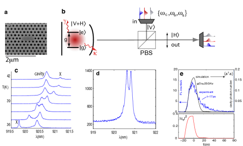
Figure 1: (a) Scanning electron micrograph of the photonic crystal cavity. (b) In the experiment, a combination of pulsed control laser (frequency $\omega_{c}$), non-resonant pulsed or continuous wave pump laser at $\omega_{e}$ above the QD exciton line, and pulsed or continuous-wave signal laser ($\omega_{s}$) is employed. The cavity is backed by a distributed Bragg reflector, effectively creating a single-sided cavity2007.Nature1 . A cross-polarized confocal microscope configuration reduces the laser background that is reflected from the sample without coupling to the cavity, which is polarized at $45^{\circ}$ to the incident laser polarization. The measurement is effectively a transmission measurement from the horizontal (H) into the vertical (V) polarization. (c) Anticrossing observed in the PL as the QD single exciton (X) is temperature-tuned through the cavity. The QD is pumped through higher-order excited states by optical excitation at $\omega_{e}$ corresponding to a wavelength of $\lambda_{e}=878$ nm. (d) The reflected intensity of a broad-band light source shows the mode splitting of the strongly coupled QD-cavity system. The reflected light is resolved on a spectrometer. (e) PL lifetime $\sim 17$ ps when the QD is tuned into the cavity and pulsed excitation wavelength $\lambda_{e}=878$ nm. The emission that is expected theoretically, based on the system parameters in (d) and a 10-ps relaxation time into the single exciton state, is shown in the solid line. The bottom panel plots the corresponding expected excited state population $|c_{e}(t)|^{2}$

We characterize the system in a confocal microscope setup in a He flow cryostat (Fig.1(b)). The photoluminescence (PL) scans in Fig.1(c) show the anticrossing between the QD-like states and the cavity-like states as the temperature is raised from 36K to 42 K, giving the polariton energies given by Eq.1. The cavity reflectivity, obtained using a white light source in the cross-polarized configuration shown in Fig.1(b), shows the same mode splitting in Fig.1(d). These spectral measurements yield the system parameters $g,\kappa$, and $\gamma$. We also characterize the system by time-resolved fluorescence after the QD is quasi-resonantly excited with 3.5-ps pulses at 878 nm. As shown in Fig.1(e), the PL decays with a characteristic time of 17 ps, as measured using a streak camera with 3 ps timing resolution. This decay closely matches a theoretical model of the cavity field and coupled QD system, as described in the Methods. The bottom panel of Fig.1(e) plots the expected excited state population $|c_{e}(t)|^{{2}}$, which shows a rise-time corresponding to the 10-ps carrier relaxation time into the lowest QD excited state.

The coupled QD/cavity system enables a strong interaction between two weak laser fields. This was previously demonstrated for two continuous-wave (cw) beams2008.Science1 . We now study the time-resolved dynamics of this interaction between cw ‘signal’ and pulsed ‘control’ fields. As illustrated in Fig.2(d), both fields are within the linewidth of the cavity resonance. In the experiment, with the QD resonant with the cavity and the control and signal beams tuned to the bottom of the transmission dip, we measure the time-resolved transmission of the control $T(c)$, the signal $T(s)$, and the signal and control $T(s+c)$ on the streak camera.

We first set the signal and control fields resonant with the tuned QD-cavity system and attenuate the power so that the average intracavity photon number is nearly zero; this corresponds to 12 nW for the cw beam and $\sim 0.2$ nW average power for the pulsed control, both measured before the objective lens. Considering a coupling efficiency into the cavity of $\eta\sim 3\%$ 2007.Nature1 , this corresponds to an average intracavity photon number of $\mathinner{\langle{a^{\dagger}a}\rangle}\sim 0.005$ for the cw beam and up to 0.025 for the pulsed beam. Here, $\mathinner{\langle{a^{\dagger}a}\rangle}$ corresponds to the instantaneous cavity photon number. Fig. 2(a) plots the curves $T(c),T(s),T(s+c)$, as well as the difference $\Delta T=T(c+s)-T(c)-T(s)$, which provides a measure of the nonlinear response of the system. Measurements for two additional sets of curves are shown in the lower plots in Fig.2(a). A stochastic simulation of the quantum master equation (see Methods) yields the cavity transmission, which is proportional to the intracavity photon numbers $n(c),n(c+s)$, and $n(s)$, as well as the nonlinear signal $\Delta n$. In fitting the data, the intensities of the pulsed and cw beams were not free parameters, but were fixed by the experimentally measured optical powers, using the same coupling efficiency $\eta$. The predicted curves are plotted in Fig.2(b) and show good agreement with the experiment. Fig.2(c) shows the theoretical value of the nonlinear coefficients $\Delta n/n(s)$ (normalized by the signal photon number) for the accessible parameter space given by signal power, control power, and the cavity parameters $\kappa,\gamma$, and $g$.

In applications such as quantum non-demolition measurements, the interaction between two frequency-detuned probe and signal fields is of interest. We therefore repeat our measurements when the control beam is detuned by up to $\Delta\lambda=0.15$ nm from the cavity frequency while the cw signal field is maintained on resonance with the cavity. Two instances are displayed in Fig.3, corresponding to detunings of $\Delta\lambda=\{0.07,0.14\}$ nm for the top and bottom plots, respectively. After the alignment is done at comparable averaged cw and pulsed powers (‘align’ curve in Fig.3(a)), the experiment is conducted with similar intracavity photon number for the cw and pulsed beams. The experiment shown uses a cw-beam and a pulsed beam with 160 nW (corresponding to $\mathinner{\langle{a^{\dagger}a}\rangle}\sim 0.07$) and $\sim 2$ nW, respectively (measured before the lens). Fig. 3(b) displays the transmitted power acquired on the streak camera, which shows a strong nonlinear increase for the pulse duration.

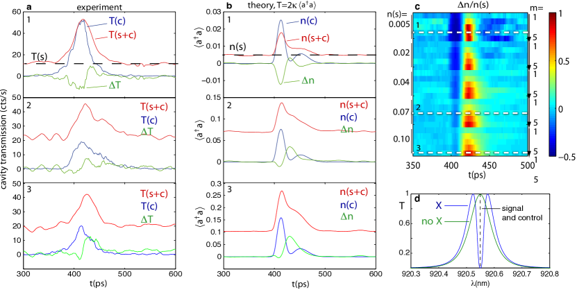
Figure 2: All-optical switching through the strongly coupled QD/cavity system. (a) Cavity transmission when the signal and control are tuned to the cavity, which is resonant with the QD. As the signal and control input powers are increased, the QD saturates and results in a net-positive nonlinear transmission. (b) Plots of the intracavity photon number $\mathinner{\langle{a^{\dagger}a}\rangle}$, which gives the transmission by $T=2\kappa\mathinner{\langle{a^{\dagger}a}\rangle}$. The calculated intracavity photon number for the control beam intracavity photon number $n(c)$, signal and control $n(s+c)$, and the differential photon number $\Delta n=n(s+c)-n(s)-n(c)$. (c) Theoretical nonlinear transmission normalized by the signal intensity for a range of signal and control fields. The signal intracavity photon number is equal to $n(s)$ across blocks where the control field is increased by a multiplier $m$ over the signal field, where $m=1,2,3,4,5$. The dashed lines correspond to the experimental conditions (1,2,3) in (a). (d) Calculated transmission with and without the QD single exciton line. The signal and control field frequencies are aligned with the QD/cavity resonance.

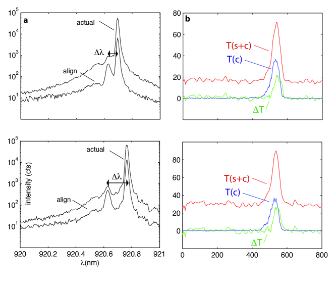
Figure 3: Nonlinear interaction between a cw-signal beam tuned to the cavity and a control pulse detuned by $\Delta\lambda$. (a) The ‘align’ curve shows the time-averaged control and the attenuated laser intensities; the ‘actual’ shows the average powers of the pulsed control and cw signal beams used in the experiment: $\sim 2$ nW for the control, 160 nW for the cw beam. (b) The control pulse results in a nonlinear transmission of the signal of $\Delta T$.

Finally, we consider how two 40-ps laser pulses, resonant with the cavity and having a relative delay of $\Delta t$ interact through the cavity. The pulse pair is generated using the delay setup of Fig.4(a). To average out interference between the two pulses, we detune them by 40 MHz and average over many pulse pairs (this detuning is very small compared to the pulse bandwidth). Numerical integration of the Master equation predicts an increased reflection when both pulses are simultaneously coupled to the cavity; this is shown for a particular choice of power in Fig.4(b). This experiment is performed on a different QD-PC cavity system with similar parameters $\{\kappa,g,\gamma\}/2\pi=\{27.2,21.2,0.1\}$ GHz; the temperature is 38K. Fig.4(c) plots the time-averaged reflected signal observed on a spectrometer for coincident pump pulses with average power of both pulses increasing from 0.3 nW to 9.2 nW before the objective lens. It is evident that for powers beyond $\sim 9$ nW, the polariton mode splitting disappears as the QD is saturated. This suggests that the QD-cavity system acts as a highly nonlinear system that increases its transmission for coincident pulses. This is what we find in Fig.4(d): the cavity transmission rises by 22% when the pulses are coincident at $\Delta t=0$. This transmission peak agrees with the theoretical prediction of a $\sim 40$ ps duration, as shown in the red curve. In the theory plot, we also observe reduced transmission at a non-zero time delay. We find that by including a pure QD dephasing term into the master equation model, the transmission dips are diminished, as observed in the experimental results. Pure QD dephasing was previously shown to play an important role in the QD-cavity system, including off-resonant interaction between the exciton and cavity mode2010.PRL.Englund . The best fit to experimental data is found for a dephasing rate of $\gamma_{d}/2\pi\approx 5$ GHz.

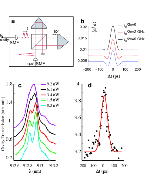
Figure 4: Interaction of two weak laser pulses through the QD/cavity system. (a) Time-delay setup for producing pulses at a separation of $\Delta t$. (b) Simulated interaction of two laser pulses, represented by the instantaneous intracavity photon number $\mathinner{\langle{a^{\dagger}a}\rangle}$ as a function of the time delay $\Delta t$ between the two 40 ps long Gaussian pulses. Curves are calculated for a set of different rates of pure QD dephasing2010.PRL.Englund , $\gamma_{d}$, which causes a reduction of the transmission dips before and after the peak. Pure dephasing also causes a blurring of the spectral normal mode splitting2010.PRL.Englund , which in turn raises the transmission for increasing $\gamma_{d}$. (c) Pump-power dependence of the cavity transmission for coincident pulses repeating at 80 MHz. (d) Signal observed when the cavity-QD system is probed with two 40 ps long pulses as a function of their delay. When the two pulses have a temporal overlap inside the cavity, the QD saturates and the overall cavity reflection increases. The power in the single of the two pulses corresponds roughly to the 3.4nW trace in (c). Best agreement is found with the theoretical plot for a pure dephasing rate $\gamma_{d}/2\pi\sim 5$ GHz.

In conclusion, we have described the interaction between time-varying control and signal fields via a strongly coupled QD/cavity system. A strong nonlinear response exists even at low intensity corresponding to mean intracavity photon numbers below one. This all-optical interaction is promising for quantum information processing with optical nonlinearities1995.PRL.Turchette-Kimble ; 1995.PRA.Chuang-Yamamoto.simple_QC ; 2005.PRA.Munro.QND_high_efficiency_abbr . The large nonlinearity may also be of use in classical all-optical signal processing2009.PRA.Mabuchi.cavity_QED_switch – for example, for the implementation of all-optical logic gates operating at the single- or few-photon level. The QD-cavity system is ideal for on-chip integration and can easily operate with repetition rates up to a tens of GHz.

Financial support was provided by the Office of Naval Research (PECASE Award), National Science Foundation, and Army Research Office. A.M. was supported by the SGF (Texas Instruments Fellow). Work was performed in part at the Stanford Nanofabrication Facility of NNIN supported by the National Science Foundation. D.E. acknowledges support by the AFOSR YIP and the Sloan Research Fellowship.

Appendix A Analytical Model

The QD is described as a two level system with a ground state $\mathinner{|{g}\rangle}$ and an excited state $\mathinner{|{e}\rangle}$. The system is characterized by a dipole decay rate $\gamma$, a cavity field decay rate $\kappa$, and a QD-cavity field coupling at the Rabi frequency $g$. The driving field is described by $\Omega(t)$. The interaction of the laser field with the coupled QD-cavity system is described by the Jaynes Cummings Hamiltonian (in a frame rotating at the laser frequency)

$$H=\Delta\omega_{c}a^{\dagger}a+\Delta\omega_{d}\sigma^{\dagger}\sigma+ig(a^{\dagger}\sigma-a\sigma^{\dagger})+i\sqrt{\kappa}\Omega(t)(a-a^{\dagger})$$ (2)

where $\Delta\omega_{c}=\omega_{c}-\omega_{l}$ and $\Delta\omega_{d}=\omega_{d}-\omega_{l}$ are respectively the cavity and dot detuning from the driving laser.

To incorporate the incoherent losses in the system we find the Master equation, given by

$$\frac{d\rho}{dt}=-i[H,\rho]+2\kappa\mathcal{L}[a]+2\gamma\mathcal{L}[\sigma]+2\gamma_{d}\mathcal{L}[\sigma^{\dagger}\sigma]$$ (3)

where $\rho$ is the density matrix of the coupled QD/cavity system and $\gamma_{d}$ is the quantum dot pure dephasing rate. $\mathcal{L}[D]$ is the Lindblad operator corresponding to a collapse operator $D$. This is used to model the incoherent decays and is given by:

$$\mathcal{L}[D]=D\rho D^{\dagger}-\frac{1}{2}D^{\dagger}D\rho-\frac{1}{2}\rho D^{\dagger}D$$ (4)

The Master equation is solved using Monte Carlo integration routines (for the mixed CW and pulsed case) and by using the numerical integration routines (for the two pulse switching case) provided in the quantum optics toolboxTanMATLAB . For the two pulse switching, we assume a Gaussian pulse-shape for the pulses.

References

- (1) Turchette, Q., Hood, C., Lange, W., Mabuchi, H., and Kimble, H. J. Phys. Rev. Lett. 75, 4710–4713 (1995).
- (2) Chuang, I. L. and Yamamoto, Y. Phys. Rev. A 52(5), 3489–3496 Nov (1995).
- (3) Imoto, N., Haus, H., and Yamamoto, Y. Phys. Rev. A 32, 2287–2292 (1985).
- (4) Wharrett, B. and Tooley, F., editors. Optical Computing. IOP Publishing, (1989).
- (5) Mabuchi, H. Phys. Rev. A 80(4), 045802 Oct (2009).
- (6) Bajcsy, M., Hofferberth, S., Balic, V., Peyronel, T., Hafezi, M., Zibrov, A. S., Vuletic, V., and Lukin, M. D. Phys. Rev. Lett. 102(20), 203902 May (2009).
- (7) Englund, D., Faraon, A., Fushman, I., Stoltz, N., Petroff, P., and Vučković, J. Nature 450(6), 857–61 (2007).
- (8) Srinivasan, K. and Painter, O. Nature 450, 862–865 December (2007).
- (9) Fushman, I., Englund, D., Faraon, A., Stoltz, N., Petroff, P., and Vuckovic, J. Science 320(5877), 769–772 (2008).
- (10) Akahane, Y., Asano, T., Song, B.-S., and Noda, S. Nature 425, 944–947 October (2003).
- (11) Toishi, M., Englund, D., Faraon, A., and Vučković, J. Opt. Express 17(17), 14618–14626 (2009).
- (12) Englund, D., Majumdar, A., Faraon, A., Mitsuru, T., Stoltz, N., Petroff, P., and Vuckovic, J. Phys. Rev. Lett. 104(7), 073904 Feb (2010).
- (13) Munro, W. J. et al. Phys. Rev. A 71(3) (2005).
- (14) Tan, S. M. J. Opt. B: Quantum Semiclass. Opt. 1, 424–432 (1999).