Intermediate Haldane phase in spin-2 quantum chains with uniaxial anisotropy

Abstract

We provide evidence of an intermediate Haldane phase in a spin-2 quantum chain. By combining effective field theory and numerical approaches, we show that the phase diagram of the proposed model includes SO(5) Haldane, intermediate Haldane, and large-$D$ phases. We determine the characteristic properties of these phases, including edge states, string order parameters, and degeneracies in the entanglement spectrum. The symmetries responsible for the degeneracy patterns observed in the entanglement spectrum are also discussed.

Introduction. Characterization of quantum phases beyond Landau’s symmetry breaking paradigm Landau-1937 is an important open problem in physics. Recently, for one-dimensional (1D) gapped phases, a classification scheme based on matrix product states (MPS) has been put forward Gu-2009 ; Pollman-2009 ; Schuch-2010 , based on the fact that ground states of 1D gapped Hamiltonians can be efficiently approximated by MPS Verstraete-2006 ; Hastings-2007 . This scheme complements the conventional approach that classifies relevant perturbations of fixed points, and sheds new light on some phases that have been extensively studied, e.g., the Haldane phase in integer-spin chains Haldane-1983 .

These developments may be helpful in order to clarify a controversial problem: the possibility of an intermediate Haldane (IH) phase (also called intermediate-$D$ phase) in quantum spin chains. This problem originated from the study of a spin-2 Heisenberg chain with uniaxial anisotropy $H=$ $\sum_{j}\vec{S}_{j}\cdot\vec{S}_{j+1}+D\sum_{j}(S_{j}^{z})^{2}$, where $D\geq 0$ (here $\vec{S}$ and $S^{z}$ are the usual spin operators). For $D=0$, the ground state is in the so-called Haldane phase. For $D\rightarrow\infty$, the ground state is in a large-$D$ phase, close to a trivial product state with $S_{j}^{z}=0$ for all $j$. Regarding the phase diagram of this model, a field theoretical approach Schulz-1986  suggests a single phase transition between the Haldane and the large-$D$ phases. On the contrary, for intermediate $D$, Oshikawa Oshikawa-1992 predicted that an IH phase may emerge between the two phases. He justified this by noticing that $S_{j}^{z}=\pm 2$ states are substantially suppressed by the $D$ term but $S_{j}^{z}=\pm 1$ states are less affected, which may lead to the formation of an effective spin-1-like Haldane phase with residual $S_{j}^{z}=\pm 1,0$ states. Nevertheless, whether such an IH phase really exists or not in the above spin-2 model (and its generalizations) remains unclear Oshikawa-1995 ; Schollwock-1996 ; Nomura-1998 ; Hatsugai-2008 ; Tonegawa-2011 .

In this work, we study a spin-2 quantum chain for which we provide sharp evidence of the existence of an IH phase. As far as we know, our results provide the clearest evidence so far in favor of the existence of such a phase in quantum spin chains. Our search for the IH phase is guided by an effective field theory, which yields a qualitative phase diagram with three quantum phases, namely: SO(5) Haldane, IH, and large-$D$ phases. The field theory also determines characteristic features of the phases, e.g., edge states in open chains and string order parameters (SOPs) den Nijs-1989 . We also determine numerically the phase diagram of the spin model, and find full agreement with the field-theory predictions. Moreover, we study the entanglement spectrum (ES) Haldane-2008 of the different phases, and confirm that the IH phase has a double degeneracy in the ES that is protected by symmetries, which distinguishes itself from the SO(5) Haldane phase with quadruple degeneracy and the large-$D$ phase without protected degeneracy. The spatial inversion, time reversal, and $(Z_{2}\times Z_{2})^{2}$ symmetries responsible for the robust degeneracy of the ES are also investigated.

Model Hamiltonian and symmetries. In this work, we consider the spin-2 quantum chain

$$H=\sum_{j}\sum_{\gamma=1}^{4}J_{\gamma}(\vec{S}_{j}\cdot\vec{S}_{j+1})^{\gamma}+D\sum_{j}(S_{j}^{z})^{2},$$ (1)

for periodic boundary condition and in the thermodynamic limit. In our case, we take $J_{1}=-\frac{11}{6},J_{2}=-\frac{31}{180},J_{3}=\frac{11}{90},J_{4}=\frac{1}{60}$, and consider the region $D\geq 0$. As we shall see, this generalization of the usual spin-2 Heisenberg chain has a number of important properties.

First, let us identify the symmetries of Eq. (1), which will turn out to be very useful for our purposes. For $D=0$, the Hamiltonian in Eq. (1) can be rewritten as $H_{D=0}=2\sum_{j}[P_{2}(j,j+1)+P_{4}(j,j+1)]$, where $P_{S_{T}}(j,j+1)$ projects onto total spin-$S_{T}$ states of neighboring sites $j$ and $j+1$. This model has SO(5) symmetry and an MPS as its exact ground state Tu-2008 ; Scalapino-1998 . To identify the SO(5) symmetry, we work in the standard $S^{z}$ basis $|m\rangle$ ($m=\pm 2,\pm 1,0$) and define SO(5) Cartan generators $L^{12}=|2\rangle\langle 2|-|-2\rangle\langle-2|$ and $L^{34}=|1\rangle\langle 1|-|-1\rangle\langle-1|$. By defining $L^{15}=\frac{1}{\sqrt{2}}(|2\rangle\langle 0|+|0\rangle\langle-2|+\mathrm{h.c.})$ and $L^{35}=\frac{1}{\sqrt{2}}(|1\rangle\langle 0|+|0\rangle\langle-1|+\mathrm{h.c.})$, the SO(5) commutation relations $[L^{ab},L^{cd}]=i\left(\delta_{ac}L^{bd}+\delta_{bd}L^{ac}-\delta_{ad}L^{bc}-\delta_{bc}L^{ad}\right)$ fix the ten generators $L^{ab}$ $(1\leq a<b\leq 5)$. For $D=0$, the Hamiltonian commutes with all ten operators $\sum_{j}L_{j}^{ab}$ and therefore has SO(5) symmetry.

For $D>0$, this SO(5) symmetry is explicitly broken down to U(1)$\times$U(1). In order to see this, we rewrite the uniaxial anisotropy as $(S^{z})^{2}=4(L^{12})^{2}+(L^{34})^{2}$. Thus, $\sum_{j}L_{j}^{12}$ and $\sum_{j}L_{j}^{34}$ commute not only with each other but also with $H$, and therefore the model has U(1)$\times$U(1) symmetry. Additionally, the Hamiltonian in Eq.(1) also has discrete symmetries, including spatial inversion, time reversal, and a set of $Z_{2}$ symmetries. These $Z_{2}$ symmetries are a consequence of the invariance under global $Z_{2}$ rotations $U^{ab}=e^{i\pi L^{ab}}$ for all $L^{ab}$. The $Z_{2}$ operators form a $(Z_{2}\times Z_{2})^{2}$ group, whose elements, without loss of generality, can be chosen as $\{\mathds{1},U^{12}\}\times\{\mathds{1},U^{15}\}\times\{\mathds{1},U^{34}\}\times\{\mathds{1},U^{35}\}$. Here we remind that these $Z_{2}$ operators preserve their form under the nonlocal Kennedy-Tasaki transformation Kennedy-1991 and also generate a hidden $(Z_{2}\times Z_{2})^{2}$ symmetry in dual space Tu-2008 .

Field-theory treatment. Even though the model in Eq. (1) looks quite complicated, its effective field theory at low energy is very simple. As we shall explain soon, this is given by the following Hamiltonian density of five Majorana fermions $\xi^{a}$ ($a=1,\ldots,5$):

$$\mathcal{H}_{\mathrm{eff}} = -iv\sum_{a=1}^{5}(\xi_{R}^{a}\partial_{x}\xi_{R}^{a}-\xi_{L}^{a}\partial_{x}\xi_{L}^{a})-im_{1}\sum_{a=1}^{2}\xi_{R}^{a}\xi_{L}^{a}$$ (2)

$$-im_{2}\sum_{a=3}^{4}\xi_{R}^{a}\xi_{L}^{a}-im_{3}\xi_{R}^{5}\xi_{L}^{5},$$

where $v$ and $m_{a}$ are velocity and masses of the Majorana fermions, and marginal four-fermion interactions have been neglected.

The strategy to derive Eq. (2) is to start from the SO(5) point $D=0$, whose effective field theory is known to be of the form given by Eq.(2) with $m_{1}=m_{2}=m_{3}<0$ Alet-2010 . In the continuum limit, the effect of the $D$ term can be taken into account by using bosonization techniques. Following Ref. Alet-2010 ; Tu-Orus-2011 , we find that $\sum_{j}(L_{j}^{12})^{2}\sim ig\int dx\sum_{a=1}^{2}\xi_{R}^{a}\xi_{L}^{a}$ and $\sum_{j}(L_{j}^{34})^{2}\sim ig\int dx\sum_{a=3}^{4}\xi_{R}^{a}\xi_{L}^{a}$, where $g<0$. By using $(S_{j}^{z})^{2}=$ $4(L_{j}^{12})^{2}+(L_{j}^{34})^{2}$, we arrive then at the expression given in Eq. (2). For $D\rightarrow 0$, we have $m_{1}-m_{3}\simeq 4(m_{2}-m_{3})\propto D$, but this relation does not hold for larger $D$ due to renormalization effects. Thus, the Majorana masses and the velocity $v$ are treated as phenomenological parameters. However, the fact that only three independent masses appear in Eq. (2), which ensures O(2)$\times$O(2) symmetry, is imposed by the U(1)$\times$U(1) symmetry of Eq. (1) since O(2)$\simeq$U(1). Moreover, the $(Z_{2}\times Z_{2})^{2}$ symmetry of Eq. (1) is also revealed by the invariance of Eq. (2) under $Z_{2}$ transformations $\xi_{R(L)}^{a}\rightarrow-\xi_{R(L)}^{a}$ Alet-2010 .

Armed with this effective field theory description, we are now in position to sketch a phase diagram for the quantum spin chain in Eq. (1). When increasing $D$ from $0$ to $\infty$, we expect that the Majorana mass $m_{3}$ is always negative in Eq. (2), while $m_{1}$ and $m_{2}$ change from negative to positive successively at two quantum critical points $D_{c_{1}}$ and $D_{c_{2}}$ ($D_{c_{1}}<D_{c_{2}}$). Both critical theories at $D_{c_{1}}$ and $D_{c_{2}}\$have two massless Majoranas, and thus are equivalent to conformal field theories with central charge $c=\frac{1}{2}\times 2=1$. For $0\leq D<D_{c_{1}}$, we call the phase ’SO(5) Haldane phase’, since its physics is captured by the SO(5) point $D=0$. For $D_{c_{1}}<D<D_{c_{2}}$, the IH phase emerges, whose characteristics will be discussed below. For $D>D_{c_{2}}$, the system enters the large-$D$ phase. A qualitative phase diagram for (1) is shown in Fig. 1.

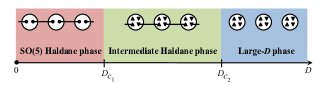
Figure 1: (Color online) Qualitative phase diagram of the spin-2 model in Eq. (1). The diagrams in the upper side correspond to the MPS structure describing the renormalization group fixed point for each phase: for low-$D$, ancillary spin-3/2 singlets are projected onto spin-2 subspaces at each physical site, thus providing an MPS for spin-2 physical particles in terms of matrices of dimension 4; for intermediate-$D$, ancillary spin-1/2 singlets, together with on-site spin-1/2 triplets $S^{z}=0$, are projected onto spin-2 at each site; for large-$D$, no singlets are projected and the state is a product state.

Similar to the spin-1 Haldane phase Affleck-1987 ; TKNg-1994 , the spin-2 IH phase has a bulk gap but exhibits gapless spin-1/2 edge excitations in open chains. Let us have a closer look at how these edge states emerge from Eq. (2). For $m_{1}>0,m_{2}<0,m_{3}<0$, our effective field theory description shares an analogy with Tsvelik’s theory Tsvelik-1990 for the spin-1 Haldane phase, formulated in terms of three Majorana fermions. On a semi-infinite chain, both theories support three Majorana zero-energy modes at the boundary, forming a fractionalized spin-1/2 edge state Lecheminant-2002 . This distinguishes the IH phase from the SO(5) Haldane phase (with spin-3/2 edge states Tu-2008 formed by five Majorana edge modes Alet-2010 ) and the large-$D$ phase (without edge states). In fact, we expect that a large family of spin-2 chains (namely, those described by a similar field theory at low energy) also support an IH phase. Interestingly, the corresponding Hamiltonians may capture the physics of some quasi-1D compounds, and thus the fractionalized edge states in the IH phase may be observed in electron spin resonance experiments by doping nonmagnetic ions Hagiwara-1990 .

The effective field theory in Eq.(2) also provides the order parameters that characterize the three gapped phases. To see this, let us view Eq.(2) as five decoupled Ising models with the Majorana mass $m\sim(T-T_{c})/T_{c}$, where $T_{c}$ is the Ising critical temperature Alet-2010 ; Tu-Orus-2011 . Defining the Ising order and disorder operators as $\sigma_{a}$ and $\mu_{a}$ $(a=1,\ldots,5)$, the SO(5) Haldane, IH, and large-$D$ phases correspond, respectively, to all five Ising models, three Ising models ($a=3,4,5$), and just one Ising model ($a=5$) in the ordered phase(s) with $\langle\sigma_{a}\rangle\neq 0$. In order to be able to distinguish these phases, we find that it is sufficient to use two SOPs

$$\mathcal{O}^{12}=\lim_{|k-j|\rightarrow\infty}\langle L_{j}^{12}\prod_{l=j}^{k-1}\exp(i\pi L_{l}^{12})L_{k}^{12}\rangle$$ (3)

and $\mathcal{O}^{34}$ (where $L^{12}$ is replaced by $L^{34}$). In the continuum limit, these SOPs are related to Ising order operators as $\mathcal{O}^{12}\sim\langle\sigma_{1}\rangle\langle\sigma_{2}\rangle,\mathcal{O}^{34}\sim\langle\sigma_{3}\rangle\langle\sigma_{4}\rangle$ Tu-Orus-2011 . Therefore, these SOPs distinguish the SO(5) Haldane ($\mathcal{O}^{12}\neq 0,\mathcal{O}^{34}\neq 0$), the IH ($\mathcal{O}^{12}=0,\mathcal{O}^{34}\neq 0$), and the large-$D$ ($\mathcal{O}^{12}=\mathcal{O}^{34}=0$) phases. As we shall see, this is very convenient in order to evaluate numerically the phase diagram of the Hamiltonian in Eq. (1).

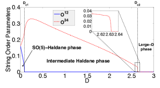
Figure 2: (Color online) String order parameters $\mathcal{O}^{12}$ and $\mathcal{O}^{34}$. They vanish smoothly at $D=D_{c_{1}}$ and $D=D_{c_{2}}$, respectively.

The solvability of the SO(5) point $D=0$ provides an intuitive picture of how these SOPs change with $D$. Starting from $D=0$, the MPS ground state of Eq. (1) has a perfect hidden string order Tu-2008 : In the $S^{z}$ basis, $\left|2\right\rangle$ and $\left|-2\right\rangle$ appear alternatively in all the configurations of the MPS if $\left|0\right\rangle$ and $\left|\pm 1\right\rangle$ are removed. Similarly, $\left|1\right\rangle$ and $\left|-1\right\rangle$ also appear alternately, if $\left|0\right\rangle$ and $\left|\pm 2\right\rangle$ are removed. This hidden string order is reflected in a nonzero value of the SOPs, $\mathcal{O}^{12}=\mathcal{O}^{34}=0.16$. When increasing $D$, the uniaxial anisotropy in Eq. (1) tends to suppress both the $\left|\pm 2\right\rangle$ and $\left|\pm 1\right\rangle$ states, but with larger suppression strength on $\left|\pm 2\right\rangle$. Thus, the string order for the $\left|\pm 2\right\rangle$ states is destroyed earlier at $D_{c_{1}}$, and an IH phase is formed with remaining string order for the $\left|\pm 1\right\rangle$ states. Here we remind that $L^{12}$ and $L^{34}$ act on $\left|\pm 2\right\rangle$ and $\left|\pm 1\right\rangle$, respectively. Therefore, we have $\mathcal{O}^{12}=0,\mathcal{O}^{34}\neq 0$ in the IH phase. When increasing $D$ further, the string order for the $\left|\pm 1\right\rangle$ states is also destroyed at $D_{c_{2}}$ and then the system enters the large-$D$ phase with $\mathcal{O}^{12}=\mathcal{O}^{34}=0$.

Phase diagram. Let us now explain our numerical results for the evaluation of the phase diagram of the model. Our technique of choice has been the so-called iTEBD algorithm Vidal-Orus-2007 . This algorithm approximates the ground-state wave function of the system in the thermodynamic limit by an MPS. To achieve this, the algorithm uses an evolution in imaginary time. The parameter that controls the accuracy of the approximation is the size of the matrices in the MPS approximation. This parameter is usually called ’bond dimension’, or $\chi$. Using this method, we have computed MPS approximations to the ground state of the Hamiltonian in Eq. (1) for different values of $D$ and $\chi$. Then, for each one of these approximations we have computed the two SOPs given in Eq. (3). In our simulations, we have seen that $\chi=40$ is enough to reproduce the phase diagram of our model with sufficient accuracy for our purposes.

Our results for the SOPs are shown in Fig. 2. We see clearly that the two SOPs distinguish the three phases, exactly as predicted by the effective field theory approach discussed above. In particular, we obtain the values for the critical points $D_{c_{1}}\sim 0.08(1)$ and $D_{c_{2}}\sim 2.63(1)$. Interestingly, we see that the IH phase actually extends through a large region in the phase diagram as compared to the SO(5) Haldane phase.

Entanglement spectrum. The concept of ES was introduced in Ref. Haldane-2008 and has proven very useful in the characterization of 1D gapped phases Pollman-2009 . From a mathematical point of view, the ES is simply the spectrum of coefficients $\xi_{\alpha}=-2\log{\lambda_{\alpha}}$, where $\lambda_{\alpha}$ are the Schmidt coefficients obtained from the Schmidt decomposition of the ground state wave function with respect to a bipartite partition in real space, $|\Psi\rangle=\sum_{\alpha}\lambda_{\alpha}|\Psi_{\alpha}^{A}\rangle|\Psi_{\alpha}^{B}\rangle$. In this equation $|\Psi_{\alpha}^{A(B)}\rangle$ are the Schmidt vectors for the $A(B)$ subsystems. Quite importantly from a numerical perspective, the iTEBD algorithm Vidal-Orus-2007 automatically renders this information, since the MPS approximation to the ground state wave function is always explicitly written in terms of the coefficients $\lambda_{\alpha}$ for all possible bipartitions of the system into two semi-infinite lines. Thus, the ES for these bipartitions can be immediately read out from the numerical MPS wave function that approximates the ground state.

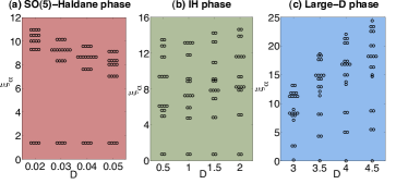
Figure 3: (Color online) First 20 coefficients $\xi_{\alpha}$ of the entanglement spectrum for representative points in the (a) SO(5) Haldane phase, (b) IH phase, and (c) large-$D$ phase.

In Fig. 3 we show our results for the first 20 coefficients $\xi_{\alpha}$ of the ES at several representative points of the three phases. As can be seen in the figure, the SO(5) Haldane phase is characterized by a quadruple degeneracy in the ES (the coefficients organize themselves in quadruplets), and the IH phase by a doubly degenerate ES (the coefficients come in duplets). As expected, the degeneracy patterns in the ES, introduced by a virtual cut, perfectly coincides with the physical edge states in these two phases. Also, we see that the large-$D$ phase has no characteristic degeneracy in the ES.

The robust degeneracies observed in the ES for the SO(5) Haldane and IH phases are protected by the symmetries of the Hamiltonian. For the IH phase, either (bond centered) spatial inversion or time reversal symmetry of Eq. (1) is sufficient to protect the doubly degenerate ES Pollman-2009 . However, the protection of the quadruply degenerate ES in the SO(5) Haldane phase is beyond the scope of these two symmetries, and is actually related to the $(Z_{2}\times Z_{2})^{2}$ symmetry. To prove this, it is sufficient to show that $(Z_{2}\times Z_{2})^{2}$ allows a nontrivial four-dimensional irreducible projective representation Gu-2009 ; Pollman-2009 . Let us identify such a projective representation by focusing on the SO(5) point $D=0$. To simplify the notation, we switch from Cartan basis to vector basis for SO(5). Using this notation, the five states in the vector basis are written as $|n^{d}\rangle$ ($d=1,\ldots,5$) and the SO(5) generators are given by $L^{ab}=i(|n^{a}\rangle\langle n^{b}|-\mathrm{h.c.})$. The SO(5) point $D=0$ has a MPS ground state $|\Psi\rangle=\sum_{\{a_{j}\}}\mathrm{Tr}(\Gamma^{a_{1}}\lambda\cdots\Gamma^{a_{N}}\lambda)|n^{a_{1}},\ldots,n^{a_{N}}\rangle$, where $\lambda=\frac{1}{2}\mathds{1}_{4\times 4}$ is the (diagonal) matrix of Schmidt coefficients, and the four-dimensional matrices $\Gamma^{a}$ at each site satisfy the Clifford algebra $\{\Gamma^{a},\Gamma^{b}\}=2\delta_{ab}$ Tu-2008 . Since $|\Psi\rangle$ is invariant under $(Z_{2}\times Z_{2})^{2}$ rotations, the local $\Gamma$ matrices must satisfy the transformation Cirac-2008

$$\sum_{d^{\prime}}(U^{ab})_{dd^{\prime}}\Gamma^{d^{\prime}}=e^{i\theta_{ab}}(V^{ab})^{\dagger}\Gamma^{d}V^{ab}.$$ (4)

By using the Clifford algebra, we obtain $\theta_{ab}=0$ and the unitaries $V^{ab}=\frac{1}{2i}[\Gamma^{a},\Gamma^{b}]$, where $\{\mathds{1},V^{12}\}\times\{\mathds{1},V^{15}\}\times\{\mathds{1},V^{34}\}\times\{\mathds{1},V^{35}\}$ is a four-dimensional irreducible projective representation of $(Z_{2}\times Z_{2})^{2}$, satisfying $\{V^{12},V^{15}\}=\{V^{34},V^{35}\}=\{V^{15},V^{35}\}=0$ and $[V^{12},V^{34}]=[V^{12},V^{35}]=[V^{15},V^{34}]=0$. Since $[V^{ab},\lambda]=0\ \forall\ V^{ab}$, the algebra of $V^{ab}$ guarantees a quadruply degenerate ES in the SO(5) Haldane phase.

Moreover, the $(Z_{2}\times Z_{2})^{2}$ symmetry also contains a two-dimensional irreducible projective representation, which protects the doubly degenerate ES in the IH phase. This indicates that the $(Z_{2}\times Z_{2})^{2}$ symmetry, besides (bond centered) spatial inversion or time reversal symmetry, also protects the IH phase. Thus, we conclude that in the presence of $(Z_{2}\times Z_{2})^{2}$ symmetry, the SO(5) Haldane and IH phases are distinct symmetry-protected topological phases Gu-2009 , which must be separated by topological phase transitions (e.g., $D_{c_{1}}$ in our model).

Conclusion. Here we have studied a spin-2 quantum chain with an IH phase. By combining effective field theory and numerical approaches we have determined the phase diagram and the characteristic properties of the phases, including edge states and SOPs. An analysis of the ES and the $(Z_{2}\times Z_{2})^{2}$ symmetry reveals that the IH and SO(5) Haldane phases are distinct topological phases protected by symmetries. Our results are clear evidence of the existence of an IH phase in quantum spin chains.

Compared to previous work Oshikawa-1992 ; Oshikawa-1995 ; Schollwock-1996 ; Nomura-1998 ; Hatsugai-2008 ; Tonegawa-2011 looking for the IH phase by considering the spin-2 Heisenberg chain (or XXZ chain) with uniaxial anisotropy, we emphasize that our starting point of the model (1) is an SO(5) Haldane phase, which is quite different from the conventional Haldane phase in the standard spin-2 Heisenberg chain and Affleck-Kennedy-Lieb-Tasaki chain Zheng-2010 ; Jiang-2010 . Nevertheless, the IH phase in our model satisfies all characteristic features suggested by Oshikawa, Oshikawa-1992 and our approach has the advantage that the guidance of a low-energy effective field theory and full characterization of phases under symmetries provide firm evidence of the existence of an IH phase.

Acknowledgements. H.H.T. acknowledges M. Cheng, H. Katsura, and Z.-X. Liu for helpful discussions. R.O. acknowledges the EU.

References

- (1) L. D. Landau, Phys. Z. Sowjetunion 11, 26 (1937).
- (2) Z.-C. Gu and X.-G. Wen, Phys. Rev. B 80, 155131 (2009); X. Chen, Z.-C. Gu, and X.-G. Wen, ibid. 83, 035107 (2011).
- (3) F. Pollmann, A. M. Turner, E. Berg, and M. Oshikawa, Phys. Rev. B 81, 064439 (2010); F. Pollmann, E. Berg, A. M. Turner, and M. Oshikawa, arXiv:0909.4059.
- (4) N. Schuch, D. Pérez-García, and J. I. Cirac, arXiv:1010.3732.
- (5) F. Verstraete and J. I. Cirac, Phys. Rev. B 73, 094423 (2006).
- (6) M. B. Hastings, J. Stat. Mech. (2007) P08024.
- (7) F. D. M. Haldane, Phys. Lett. A 93, 464 (1983); Phys. Rev. Lett. 50, 1153 (1983).
- (8) H. J. Schulz, Phys. Rev. B 34, 6372 (1986).
- (9) M. Oshikawa, J. Phys.: Condens. Matter 4, 7469 (1992).
- (10) M. Oshikawa, M. Yamanaka, and S. Miyashita, cond-mat/9507098.
- (11) U. Schollwöck and T. Jolicœur, Europhys. Lett. 30, 493 (1995); U. Schollwöck, O. Golinelli, and T. Jolicœur, Phys. Rev. B 54, 4038 (1996); H. Aschauer and Schollwöck, ibid. 58, 359 (1998).
- (12) K. Nomura and A. Kitazawa, J. Phys. A 31, 7341 (1998).
- (13) T. Hirano, H. Katsura, and Y. Hatsugai, Phys. Rev. B 77, 094431 (2008).
- (14) T. Tonegawa, K. Okamoto, H. Nakano, T. Sakai, K. Nomura, and M. Kaburagi, J. Phys. Soc. Jpn. 80, 043001 (2011); K. Okamoto, T. Tonegawa, H. Nakano, T. Sakai, K. Nomura, M. Kaburagi, arXiv:1101.2799.
- (15) M. den Nijs and K. Rommelse, Phys. Rev. B 40, 4709 (1989).
- (16) H. Li and F. D. M. Haldane, Phys. Rev. Lett. 101, 010504 (2008).
- (17) H.-H. Tu, G.-M. Zhang, and T. Xiang, Phys. Rev. B 78, 094404 (2008); J. Phys. A 41, 415201 (2008).
- (18) D. Scalapino, S.-C. Zhang, and W. Hanke, Phys. Rev. B 58, 443 (1998).
- (19) T. Kennedy and H. Tasaki, Phys. Rev. B 45, 304 (1992).
- (20) F. Alet, S. Capponi, H. Nonne, P. Lecheminant, and I. P. McCulloch, Phys. Rev. B 83, 060407(R) (2011).
- (21) H.-H. Tu and R. Orús, Phys. Rev. Lett. 107, 077204 (2011).
- (22) I. Affleck, T. Kennedy, E. H. Lieb, and H. Tasaki, Phys. Rev. Lett. 59, 799 (1987).
- (23) T.-K. Ng, Phys. Rev. B 50, 555 (1994).
- (24) A. M. Tsvelik, Phys. Rev. B 42, 10499 (1990).
- (25) P. Lecheminant and E. Orignac, Phys. Rev. B 65, 174406 (2002).
- (26) M. Hagiwara, K. Katsumata, I. Affleck, B. I. Halperin, and J. P. Renard, Phys. Rev. Lett. 65, 3181 (1990).
- (27) G. Vidal, Phys. Rev. Lett. 98, 070201 (2007); R. Orús and G. Vidal, Phys. Rev. B 78, 155117 (2008).
- (28) D. Pérez-García, M. M. Wolf, M. Sanz, F. Verstraete, and J. I. Cirac, Phys. Rev. Lett. 100, 167202 (2008).
- (29) D. Zheng, G.-M. Zhang, T. Xiang, and D.-H. Lee, Phys. Rev. B 83, 014409 (2011).
- (30) J. Zang, H.-C. Jiang, Z.-Y. Weng, and S.-C. Zhang, Phys. Rev. B 81, 224430 (2010); H.-C. Jiang, S. Rachel, Z.-Y. Weng, S.-C. Zhang, and Z. Wang, Phys. Rev. B 82, 220403(R) (2010).