Amplitude control of quantum interference

Abstract

Usually, the oscillations of interference effects are controlled by relative phases. We show that varying the amplitudes of quantum waves, for instance by changing the reflectivity of beam splitters, can also lead to quantum oscillations and even to Bell violations of local realism. We first study theoretically a generalization of the Hong-Ou-Mandel experiment to arbitrary source numbers and beam splitter transmittivity. We then consider a Bell type experiment with two independent sources, and find strong violations of local realism for arbitrarily large source number $N$; for small $N$, one operator measures essentially the relative phase of the sources and the other their intensities. Since, experimentally, one can measure the parity of the number of atoms in an optical lattice more easily than the number itself, we assume that the detectors measure parity.

I. Introduction. In classical and quantum physics, the usual control parameter of interference phenomena is the phase. For instance, the interference pattern observed on a screen occurs because, at the various points of the screen, the fields radiated from two coherent sources have variable phase differences. In classical physics, this is explained by the usual Fresnel construction in the complex plane, where the phase difference controls the angle between two vectors, leading to oscillations as a function of this phase Born-and-Wolf ; by contrast, no oscillation is expected when the amplitude of the vectors is changed at constant phase. In quantum physics, the phase also often plays the role of a parameter controlling oscillations, e.g., at the output of a Mach-Zhender interferometer Mach crossed by a series of single particles. Another example is the oscillations of correlation functions leading to the observation of violations of Bell inequalities, where the control parameters are the rotation of linear analyzers defining the relative phase of two circular polarizations Freedman . The purpose of this article is to show that, in quantum physics, changing the amplitudes can also lead to strong oscillations and quantum interference effects. These oscillations occur with bosonic systems, which can be described either as fields or systems of particles. Curiously, they are due to the particle character of the quantum system, and disappear when the granularity of the field vanishes and when detectors measure continuous intensity variables semiclassical .

A motivation for this study is given by recent experiments made with Bose-Einstein condensates and atomic interferometers with ultracold gases AtomInterf1 . Atom beam splitters AtomInterf1 may either involve Bragg scattering Bragg1 ; Bragg2 or be formed by the use of radio-frequency-induced adiabatic double-well potentials Kruger . In the latter case, the splitting of one condensate into two parts can easily be adjusted to provide various given ratios between their populations, corresponding naturally to beam splitters with variable transmission and reflection coefficients. Moroever, recent experiments using optical lattices have shown that, while counting individual particles may be difficult, one can much more easily measure the parity of the number of particles trapped in a potential well Greiner ; Cheneau . The reason is that, on each lattice site, atoms recombine by pairs and form molecules escaping the trap. This is why we study the effect of beam splitters with variable transmittivity on the parity of the number of particles in each output beam. While we emphasize the use of ultracold gases in the experiments we propose, it may be possible to produce the necessary Fock states by photonic methods Hof ; Wang ; Geremia ; Dots .

In this paper we discuss two possible experiments: one with two sources and one beam splitter and two detectors, the other with more beam splitters and detectors and illustrating quantum non-locality. The first is a simple generalization of the Hong-Ou-Mandel (HOM) Hong-Ou-Mandel experiment in which two bosons (photons or atoms) interfere at a beam splitter, resulting in the absence of any possible coincidence counts in the two detectors. Here we consider arbitrary source populations and the effect of changing the reflectivity of the beam splitter. In the second, we extend violations of the Bell inequalities, found previously EuroLM ; FL2 with Fock-state condensates, to cases where the reflectivities are used as control parameters; indeed we find that the violations actually exceed those obtained by controlling phase shifts.

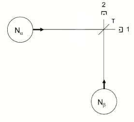
Figure 1: $N_{\alpha},N_{\beta}$ bosons proceed from the sources to a beam splitter, followed by two detectors 1 and 2, where $m_{1}$ and $m_{2}$ particles are detected. The beam splitter has an adjustable transmission coefficient, $T$, not necessarily set to $1/2$.

II. Generalized HOM Effect and Parity. We generalize the HOM effect to an arbitrary number of photons and to arbitrary $T$ and $R=1-T$, using the same formalism as in foundLM (where R and T were each taken equal to 1/2). We also study whether such a generalized HOM experiment (GHOM) can be performed if only the measurement of the parity of the numbers of the particles at the detectors is available. The device is shown in Fig. 1.

Before the beams of bosons cross the beam splitter, they are described by the quantum state

$$\left|N_{\alpha},N_{\beta}\right\rangle=\frac{1}{\sqrt{N_{\alpha}!N_{\beta}!}}a_{\alpha}^{\dagger N_{\alpha}}a_{\beta}^{\dagger N_{\beta}}\left|\text{0}\right\rangle$$ (1)

The destruction operators associated with the two output beams (and detectors) are

$$a_{1}=\left(\sqrt{T}a_{\alpha}+i\sqrt{R}a_{\beta}\right);\qquad a_{2}=\left(i\sqrt{R}a_{\alpha}+\sqrt{T}a_{\beta}\right)$$ (2)

The amplitude for finding $m_{1},m_{2}$ particles in the detectors given sources with $N_{\alpha},N_{\beta}$ particles is

$$C_{m_{1}m_{2}}(N_{\alpha},N_{\beta}) =\frac{1}{\sqrt{m_{1}!m_{2}!N_{\alpha}!N_{\beta}!}}\left\langle 0\right|a_{1}^{m_{1}}a_{2}^{m_{2}}a_{\alpha}^{\dagger N_{\alpha}}a_{\beta}^{\dagger N_{\beta}}\left|0\right\rangle$$

$$=\frac{\sqrt{N_{\alpha}!N_{\beta}!}}{\sqrt{m_{1}!m_{2}!}}\sum_{p,q}\frac{m_{1}!m_{2}!\left(\sqrt{T}\right)^{p+m_{2}-q}\left(i\sqrt{R}\right)^{q+m_{1}-p}}{p!(m_{1}-p)!q!(m_{2}-q)!}\delta_{p+q,N_{\alpha}}\delta_{m_{1}+m_{2}-p-q,N_{\beta}}$$

$$=\sqrt{\frac{N_{\alpha}!N_{\beta}!}{m_{1}!m_{2}!}}\int_{-\pi}^{\pi}\frac{d\phi}{2\pi}e^{-iN_{\alpha}\phi}\left(\sqrt{T}e^{i\phi}+i\sqrt{R}\right)^{m_{1}}\left(i\sqrt{R}e^{i\phi}+\sqrt{T}\right)^{m_{2}}$$ (3)

where we have replaced the first $\delta$-function of the second line in Eq. (3) by $\int\frac{d\phi}{2\pi}e^{i\phi(p+q-N_{\alpha})}$, and have redone the sum. The square of the modulus of this expression contains an integral over two variables $\phi$ and $\phi^{\prime}$; if we make the changes of variables $\lambda=(\phi+\phi^{\prime}+\pi)/2$ ; $\Lambda=(\phi-\phi^{\prime})/2$, we find for the probability the expression:

$$P(m_{1},m_{2}) = \frac{N_{\alpha}!N_{\beta}!}{m_{1}!m_{2}!}\int_{-\pi}^{\pi}\frac{d\lambda}{2\pi}\int_{-\pi}^{\pi}\frac{d\Lambda}{2\pi}e^{-i(N_{\alpha}-N_{\beta})\Lambda}\left[Te^{i\Lambda}+Re^{-i\Lambda}-2\sqrt{TR}\cos\lambda\right]^{m_{1}}$$ (5)

$$\times\left[Re^{i\Lambda}+Te^{-i\Lambda}+2\sqrt{TR}\cos\lambda\right]^{m_{2}}$$

That this probability shows interference effects is seen in Fig. 2(a) for the case of $T=R=1/2$ and $N_{\alpha}=N_{\beta}$. Only pairs of particles reach either detector. If we define the parity as $\left\langle p_{m_{1}}\right\rangle=\sum_{m_{1}}(-1)^{m_{1}}P(m_{1},N-m_{1})$ we find unity for the case shown in Fig. 2(a), a first indication that parity is a useful indicator of interference effects. For general values of $T$ and $R=1-T$ we find

$$\left\langle p_{m_{1}}\right\rangle =\frac{2^{N}N_{\alpha}!N_{\beta}!}{N!}\int_{-\pi}^{\pi}\frac{d\lambda}{2\pi}\int_{-\pi}^{\pi}\frac{d\Lambda}{2\pi}e^{-i(N_{\alpha}-N_{\beta})\Lambda}\left[i\left(R-T\right)\sin\Lambda+2\sqrt{TR}\cos\lambda\right]^{N}$$

$$=2^{N}N_{\alpha}!N_{\beta}!\sum_{p=0}^{N}\frac{(-1)^{(p-N_{\alpha}+N_{\beta})/2}(R-T)^{p}\left(\sqrt{TR}\right)^{N-p}y(N-p)y(N_{\alpha}-N_{\beta}+p)}{2^{p}\left(\frac{N-p}{2}\right)!^{2}\left(\frac{N_{\alpha}-N_{\beta}+p}{2}\right)!\left(\frac{p-N_{a}+N_{\beta}}{2}\right)!}$$ (6)

where $y(x)=\frac{1}{2}(1+(-1)^{x})$. The second line of (6) comes from expanding the integrand in Eq. (5) and integrating term by term. For the case $T=R=1/2$ this reduces to $\left\langle p_{m_{1}}\right\rangle_{N_{\alpha},N_{\beta}}=\delta_{N_{\alpha},N_{\beta}}$. (While the plots of $P(m_{1},m_{2})$ for $N_{\alpha}\neq N_{\beta}$ continue to show interference effects, the probability for finding even values of $m_{1}$ is the same as that for finding odd values, so that parity does not show the interference in that case.)

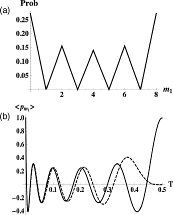
Figure 2: (a) The probability of Eq. (5) vs. $m_{1}$ for $N_{\alpha}=4,\text{~{}}N_{\beta}=4$ and $T=R=1/2$ illustrating the rule that, if an even number of particles enters each side of the beam splitter, an even number must emerge from each side. (b) Parity average versus $T$ for $N_{\alpha}=N_{\beta}=10$ (solid) and $N_{\alpha}=12,$ $N_{\beta}=8$ (dashed).

In Fig. 2(b) we show $\left\langle p_{m_{1}}\right\rangle$ versus $T$ for equal and unequal $N_{\alpha}$ and $N_{\beta}$. Note the values are much the same except near $T=0.5.$ To get an understanding of the oscillations of the parity with $T$ and how they reveal the interference effects, consider the simpler situations where $N_{\alpha}$ and $N_{\beta}$ are small. For $N_{\alpha}=2$, $N_{\beta}=1$ we have

$$a_{\alpha}^{\dagger 2}a_{\beta}^{\dagger} =\frac{1}{2^{3/2}}\left[T\sqrt{R}a_{1}^{\dagger 3}+\sqrt{T}(T-2R)a_{1}^{\dagger 2}a_{2}^{\dagger}\right.$$

$$\left.+\sqrt{R}(R-2T)a_{1}^{\dagger}a_{2}^{\dagger 2}-Ra_{2}^{\dagger 2}\right]$$ (7)

From this we see that negative parity is favored when $T=2R$ , ($T=0.66)$ and positive for $R=2T$, ($T=0.33)$ and this is very close to what we find by explicit calculation. Again we have cancellation for the various possible ways two particles can get to detector 1 and one to detector 2 and vice versa. These maxima and minima estimates are not exact since the parity depends on all processes, not just a subset. Sanaka et al Sanaka have considered the special case where $N_{\alpha}=n$ and $N_{\beta}=1$ and shown that $P(1,n)$ of Eq. (4) vanishes when $R=n/(n+1)$ allowing filtering of $n$-particle states out of an input beam. If parity is more easily measured than actual detector counts, one could argue that the same is true of source numbers. For the case $T=1/2$ a random distribution of source numbers $N_{\alpha},N_{\beta}$ will favor even parity because of the occasional occurrence of terms where $N_{\alpha}=N_{\beta}$. With a binomial source distribution, where the total number of particles is known to be $N$, we have a source-averaged parity of

$$\left\langle p_{m_{1}}\right\rangle = \sum_{N_{\alpha=0}}^{N}\frac{N!\delta_{N_{\alpha},N-N_{\alpha}}}{{2}^{N}N_{\alpha}!(N-N_{\alpha})!}=\begin{cases}\frac{N!}{2^{N}(N/2)!^{2}}\\ 0\end{cases}$$ (8)

where the top line holds for $N$ even and the bottom for $N$ odd. (The latter result holds because we cannot have $N_{\alpha}=N_{\beta}$ with odd total $N$). An analogous result will hold for any source distribution. If we can count the parity of the total source distribution, we can always guarantee to see the interference result. As $N$ increases the average parity decreases, but the method works well for small $N.$ Analogous arguments can be made for $T\neq 1/2.$

Parity oscillations, as a function of $T$, therefore provide a useful signature of the GHOM quantum effect. We now show that the same ideas can lead to strong violations of the Bell-Clauser-Horne-Shimony-Holt (BCHSH) inequalities Bell ; CHSH .

III. Violating BCHSH inequalities by varying transmission coefficients. The interferometer we analyze is shown in Fig. 3. We have analyzed this device previously FL2 ; EuroLM with variations of the phase shifters and have seen that the Bell inequalities may be violated for arbitrarially large $N$. In the present analysis we want to allow the experimenters, Alice and Bob, to vary the transmission coefficients $T_{1}$ and $T_{2}$ at their detectors.

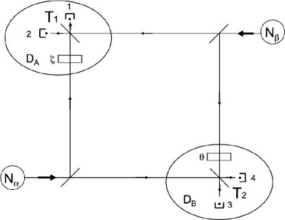
Figure 3: Two Fock states, with populations $N_{\alpha}$ and $N_{\beta}$, divide at beam splitters, and are made to interfere in two regions $D_{A}$ and $D_{B}$, with counting in detectors 1 and 2 in the former, 3 and 4 in the latter. The phase shifts, $\zeta$ and $\theta$, are zero in this analysis. The transmission coefficients at $D_{A}$ and $D_{B}$, $T_{1}$ and $T_{2}$, respectively, are varied. The transmission coefficients at the sources remain set at 1/2.

The corresponding operators are

$$\begin{array}[]{l}a_{1}=\frac{i}{\sqrt{2}}\left[\sqrt{T_{1}}a_{\alpha}+\sqrt{R_{1}}a_{\beta}\right]\text{;\ }a_{2}=\frac{-1}{\sqrt{2}}\left[\sqrt{R_{1}}a_{\alpha}-\sqrt{T_{1}}a_{\beta}\right]\\ a_{3}=\frac{i}{\sqrt{2}}\left[\sqrt{R_{2}}a_{\alpha}+\sqrt{T_{2}}a_{\beta}\right]\text{;\ }a_{4}=\frac{1}{\sqrt{2}}\left[\sqrt{T_{2}}a_{\alpha}-\sqrt{R_{2}}a_{\beta}\right]\end{array}$$ (9)

or generally $a_{i}=u_{i}a_{\alpha}+v_{i}a_{\beta}$. We consider the case where the sources are equal: $N_{\alpha}=N_{\beta}=N/2$. By proceeding as we did above we find the probability for finding $\{m_{1},m_{2},m_{3},m\}$ is

$$P_{m_{1}m_{2}m_{3}m_{4}} =\frac{(N/2)!^{2}}{m_{1}!\cdots m_{4}!}\int\frac{d\phi^{\prime}}{2\pi}e^{iN\phi^{\prime}/2}$$

$$\times\int_{-\pi}^{\pi}\frac{d\phi}{2\pi}e^{-iN\phi/2}\prod_{i=1}^{4}\Omega_{i}^{m_{i}}$$ (10)

where

$$\Omega_{i}=\left(u_{i}^{*}e^{-i\phi^{\prime}}+v_{i}^{*}\right)\left(u_{i}e^{i\phi}+v_{i}\right)$$ (11)

For the parity correlation we want the average of $\mathcal{AB}$ where $\mathcal{A}=(-1)^{m_{2}}$ and $\mathcal{B}=(-1)^{m_{4}}$. After a straightforward calculation we find

$$\left\langle\mathcal{AB}\right\rangle=\left(\frac{N}{2}!\right)^{2}\sum_{p=0,2,}^{N}\frac{(-1)^{p/2}\Delta T^{p}\tau^{N-p}}{(\frac{p}{2})!^{2}(\frac{N-p}{2})!^{2}}$$ (12)

where

$$\Delta T = T_{1}-T_{2}$$ (13)

$$\tau = \sqrt{T_{1}(1-T_{1})}+\sqrt{T_{2}(1-T_{2})}$$ (14)

If we plot $\left\langle\mathcal{AB}\right\rangle$ as a function of $T_{1}$ and $T_{2}$ (Fig. 4) we find oscillations analogous to to those in Fig. 2.

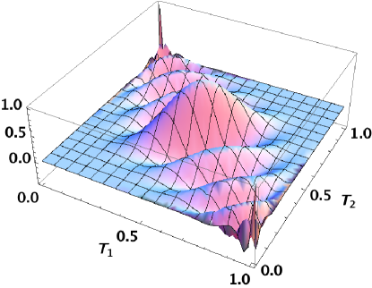
Figure 4: (Color online) Oscillations in $\left\langle\mathcal{AB}\right\rangle$ as a function of $T_{1}$ and $T_{2}$. $N_{\alpha}=N_{\beta}=10$.

The BCHSH inequality CHSH is

$$Q=\left\langle\mathcal{AB}\right\rangle+\left\langle\mathcal{AB}^{\prime}\right\rangle+\left\langle\mathcal{A}^{\prime}\mathcal{B}\right\rangle-\left\langle\mathcal{A}^{\prime}\mathcal{B}^{\prime}\right\rangle\leq 2$$ (15)

where the primes refer to using the four pairs of variables $T_{1}$, $T_{2},$ $T_{1}^{\prime}$, and $T_{2}^{\prime}$. For $N=2$ we find a maximum of $Q=2.31$ for the set of $T$ values $\{0.57,$ 0.43, 0.06, 0.94}. As $N$ increases the optimal $Q$ increases and $T$ values move close to $1/2$. A plot is shown in Fig. 5

Figure 5: BCHSH Quantity $Q$ vs. $N$. The solid line is the result of varying the transmission coefficients. The dashed line compares the resuts from Refs. EuroLM ; FL2 in which the phase shifts were varied.

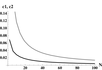
Figure 6: The maximization parameters $c_{1}$ (in black) and $c_{2}$ (in gray) giving the differences of the transmission coefficients from 0.5 at maximum.

The $Q$ value found at $N=100$ is $2.54$ with the $T$ set of {0.486, 0.504, 0.514, 0.486}. The maximum possible value extrapolates to $\sim 2.56$ at large $N.$ The $T$ values range around 0.5 in terms of just two variables $c_{1}$ and $c_{2}$, as follows $\{T_{1},T_{2},T_{1}^{\prime},T_{2}^{\prime}\}=\{0.5-c_{1},0.5+c_{1},0.5+c_{2},0.5-c_{2}\}$. (See Fig. 6.) For very small $N$ we have $T_{1}^{\prime}$, and $T_{2}^{\prime}$ near 0 and 1, respectively. The four detectors register $m_{1}\cdots m_{4}$ from which, in a second step, one calculates two parities. If $T_{1}$ and $T_{2}$ are $1/2$, no detector can distinguish the source from which the particles originate; the ratios between the $m_{i}$ provide, classically, the relative phase of the sources. If the $T$ values are 0 or 1, the source populations are directly measured. Thus for very small $N$ our scheme involves a combination of experiments where Alice and Bob essentially measure, either the relative phase (with $T_{1}$ and $T_{2}$ near $1/2$), or the source numbers (with $T_{1}$ and $T_{2}$ near 0 or 1). The conjugate variables here are numbers and phase, instead of the usual quadrature operators in Bell violations.

It is interesting to compare (see Fig. 5) our results to the case in Refs. EuroLM ; FL2 where we varied the phase shifts ($\zeta$ and $\theta$ in Fig. 3). There we had $Q=2.41$ at $N=2$ with $Q$ then decreasing until it reached a limit of $2.32$ at large N. With phase-angle variation, $Q$ decreases with $N$, but with $T$ variation it increases with $N$ and becomes much larger than occurred with the angle variation.

We tried varying both angles and transmission coefficients simultaneously using four pairs of variables $\{T_{1},\zeta\}$, $\{T_{2},\theta\},$ $\{T_{1}^{\prime},\zeta^{\prime}\}$, and $\{T_{2}^{\prime},\theta^{\prime}\}$. We never succeeded in improving the results.

Parity, which is a possible measurable variable in ultra-cold gases, provides a useful signature of quantum interference and non-local effects. The more surprising result of our analysis is that, even for systems with a large number of particles, the probability of particle transmission provides a powerful way of observing these phenomena. In studying the GHOM effect we find curious oscillations of the parity as $T$ is varied. In Bell violations the wave amplitude variation actually achieves greater violations than by changes in phase.

Laboratoire Kastler Brossel is “UMR 8552 du CNRS, de l’ENS, et de l’Université Pierre et Marie Curie”.

References

- (1) E. Hecht, Optics, Addison-Wesley; 4th ed. (San Francisco, 2002).
- (2) E. Mach, The Principles of Physical Optics. Dover, 2003.
- (3) S. J. Freedman and J. F. Clauser, Phys. Rev. Lett. 28, 938 (1972).
- (4) They even disappear in a semi-quantum model where individual particles cross or bounce on beam splitters with probabilities given by field intensities.
- (5) A. D. Cronin, J. Schmiedmayer, and D. E. Pritchard, Rev. Mod. Phys. 81, 1051 (2009).
- (6) Y. B. Ovchinnikov, J. H. Muller, M. R. Doery, E. J. D. Vredenbregt, K. Helmerson, S. L. Rolston, W. D. Phillips, Phys. Rev. Lett. 83, 284 (1999).
- (7) J. Sebby-Strabley, B. L. Brown, M. Anderlini, P. J. Lee, W. D. Phillips, J. V. Porto, P. R. Johnson, Phys. Rev. Lett. 98, 200405 (2007).
- (8) T. Schumm, S. Hofferberth, L. M. Andersson, S. Wildermuth, S. Groth, I. Bar-Joseph, J. Schmiedmayer, and P. Krüger, Nature Physics 1, 57 (2005).
- (9) W. S. Bakr, J. I. Gillen, A. Peng, S. Fölling, and M. Greiner, Nature 462, 74 (1969).
- (10) J. F. Sherson, C. Weitenberg, M. Endres, M. Cheneau, I. Bloch, and S. Kuhr, Nature 467, 68 (2010).
- (11) M. Hofheinz, E. M. Weig, M. Ansmann, R. C. Bialczak, E. Lucero, M. Neeley, A. D. O’Connell, H. Wang, J, M. Martinis, and A. N. Cleland, Nature 454, 310 (2008).
- (12) H. Wang, M. Hofheinz, M. Ansmann, R. C. Bialczak, E. Lucero, M. Neeley, A. D. O’Connell, J. Wenner, A. N. Cleland, J. M. Martinis, Phys. Rev. Lett. 101 240401 (2008).
- (13) J. M. Geremia, Phys. Rev. Lett. 97, 073601 (2009).
- (14) I. Dotsenko, M. Mirrahimi, M. Brune, S. Haroche, J.-M. Raimond, and P. Rouchon, Phys. Rev. A 80, 013805 (2009).
- (15) C. K. Hong, Z. Y. Ou, and L. Mandel, Phys. Rev. Lett. 59, 2044 (1987).
- (16) F. Laloë and W. J. Mullin, Eur. Phys. J. B 70, 377 (2009).
- (17) W. J. Mullin and F. Laloë, Phys. Rev. A 78, 061605R (2008).
- (18) F. Laloë and W. J. Mullin, Found. Phys. 42, 53 (2012).
- (19) K. Sanaka, K. J. Rush, and A. Zeilinger, Phys. Rev. Lett. 96, 083601 (2006).
- (20) J. S. Bell, Physics 1, 195 (1964), reprinted in J. S. Bell, Speakable and unspeakable in quantum mechanics, (Cambridge University Press , Cambridge, 1987).
- (21) J. F. Clauser, M. A. Horne, A. Shimony and R. A. Holt, Phys. Rev. Lett. 23, 880 (1969).