Squeeze-and-Breathe Evolutionary Monte Carlo Optimisation with Local Search Acceleration and its application to parameter fitting

Abstract

Motivation: Estimating parameters from data is a key stage of the modelling process, particularly in biological systems where many parameters need to be estimated from sparse and noisy data sets. Over the years, a variety of heuristics have been proposed to solve this complex optimisation problem, with good results in some cases yet with limitations in the biological setting.
Results: In this work, we develop an algorithm for model parameter fitting that combines ideas from evolutionary algorithms, sequential Monte Carlo and direct search optimisation. Our method performs well even when the order of magnitude and/or the range of the parameters is unknown. The method refines iteratively a sequence of parameter distributions through local optimisation combined with partial resampling from a historical prior defined over the support of all previous iterations. We exemplify our method with biological models using both simulated and real experimental data and estimate the parameters efficiently even in the absence of a priori knowledge about the parameters.
Availability: Matlab code available from the authors upon request.

1 Introduction

The increasing drive towards quantitative technologies in Biology has brought with it a renewed interest in the modeling of biological systems. Models of biological systems and other complex phenomena are generally nonlinear with uncertain parameters, many of which are often unknown and/or unmeasurable (Edelstein-Keshet, 1988; Alon, 2007). Crucially, the values of the parameters dictate not only the quantitative but also the qualitative behaviour of such models (Strogatz, 1994; Brown and Sethna, 2003). A fundamental task in quantitative and systems biology is to use experimental data to infer parameter values that minimise the discrepancy between the behaviour of the model and experimental observations. The parameters thus obtained can then be cross-validated against unused data before employing the fitted model as a predictive tool (Alon, 2007). Ideally, this process could help close the modelling-experiment loop by: suggesting specific experimental measurements; identifying relevant parameters to be measured; or discriminating between alternative models (Gutenkunst et al., 2007; Toni and Stumpf, 2009; Yates et al., 2001).

The problem of parameter estimation and data fitting is classically posed as the minimisation of a cost function (i.e., the error) (Gershenfeld, 1999). In the case of overdetermined linear systems with quadratic error functions, this problem leads to least-square solutions, convex optimisations that can be solved efficiently and globally based on the singular value decomposition of the covariance matrix of the data (Lawson and Hanson, 1995). However, data fitting in nonlinear systems with small amounts of data remains difficult, as it usually leads to non-convex optimisations with many local minima (Brewer et al., 2008).

A classic case in biological modeling is the description of the time evolution of a system through ordinary differential equations (ODEs), usually based on mechanistic functional forms. Examples include models of biochemical reactions, infectious spread and neuronal dynamics (Anderson and May, 1992; Edelstein-Keshet, 1988). Typically, optimal parameters of the nonlinear ODEs must be inferred from experimental time courses but the associated optimisation is far from straightforward. Standard optimisation techniques that require an explicit cost function are unsuitable for this problem due to the difficulty to obtain full analytical solutions for nonlinear ODEs (Brown and Sethna, 2003; Chen et al., 2010; Papachristodoulou and Recht, 2007). Spline-based methods, which approximate the solution though an implicit integration of the differential equation (Brewer et al., 2008), require linearity in the parameters and are therefore not applicable to models with nonlinear parameter dependencies, e.g. Michaelis-Menten and Hill kinetics.

Implicit techniques, such as direct search methods (Powell, 1998), Simulated Annealing (Kirkpatrick et al., 1983), Evolutionary Algorithms (Mitchell, 1997; Runarsson and Yao, 2000) or Sequential Monte Carlo (Sisson et al., 2007), do not require an explicit cost function. However, if as is usually the case, the cost function is a complicated (hyper)surface in parameter space with many local minima, gradient and direct search methods tend to get trapped in local minima due to their use of local information. Although still a local method, Simulated Annealing alleviates some of the problems related to local minima through the use of stochasticity. However, this comes at the cost of high computational overhead and slow convergence and, yet, with no guarantee of finding the global minimum.

Instead of an optimisation based on local criteria, Evolutionary Algorithms (EA) produce an ensemble of possible answers and evolve them globally through random mutation and cross-over followed by ranking and culling of the worst solutions (Mitchell, 1997; Runarsson and Yao, 2000; Schwefel, 1995). This heuristic has been shown to provide an efficient protocol for parameter fitting in the life sciences (Moles et al., 2003; Zi and Klipp, 2006). However, EA methods can be inefficient when the feasible region in parameter space is too large, a case typical of models with large uncertainty in the parameters.

Probabilistic methods, such as Sequential Monte-Carlo (SMC) (Sisson et al., 2007), propose a different conceptual framework. Rather than finding a unique optimal parameter set, SMC maps a prior probability distribution of the parameters onto a posterior constructed from samples with low errors until reaching a converged posterior. Recently, SMC has been combined with Approximate Bayesian Computation (ABC) and applied to data fitting and model selection (Toni et al., 2009). However, methods such as ABC-SMC are not only computationally expensive but also require that the starting prior include the true value of the parameters. This requirement dents its applicability to many biological models, in which not even the order of magnitude of the parameters is known. In that case, the support of the starting priors must be made overly large (leading to extremely slow convergence) in order to avoid the risk of excluding the true parameter value from the search space.

In this work, we present an optimisation algorithm for data fitting that takes inspiration from EA, SMC and direct search optimisation. Our method iterates and refines samples from a probability distribution of the parameters in a ’squeeze-and-breathe’ sequence. At each iteration the probability distribution is ‘squeezed’ by the consecutive application of local optimisation followed by ranking and culling of the local optima. The parameter distribution is then allowed to ‘breathe’ through a random update from a historical prior that includes the union of all past supports of the solutions (Fig. 1). This iteration proceeds until convergence of the distribution of solutions and their average error. A key feature of the algorithm is the accelerated step-to-step convergence through a combination of local optimisation and of culling of local solutions. Importantly, the method can also find parameters that lie outside of the range of the initial prior, and can deal with parameter values that extend across several orders of magnitude. We now provide definitions and a full description of our algorithm and showcase its applicability to different biological models of interest.

2 Algorithm

2.1 Formulation of the problem

Let $\mathbf{X}(t)=[x_{1}(t),\dots,x_{d}(t)]$ denote the state of a system with $d$ variables at time $t$. The time evolution of the state is described by a system of (possibly nonlinear) ODEs:

$$\dot{\mathbf{X}}=f(\mathbf{X},t;\,\boldsymbol{\theta}).$$ (1)

Here $\boldsymbol{\theta}=[\theta_{1},\dots,\theta_{N}]$ is the vector of $N$ parameters of our model.

The experimental data set is formed by $M$ observations of some of the variables of the system:

$$\mathcal{D}=\left\{\widetilde{\mathbf{X}}(t_{i})\,|\,i=1,\dots,M\right\}.$$ (2)

Ideally, $M>2N+1$ since $2N+1$ experiments are enough for unequivocal identification of an ODE model with $N$ parameters when no measurement error is present (Sontag, 2002).

The cost function (i.e., the error) to be minimised is:

$$E_{\mathcal{D}}(\boldsymbol{\theta})=\sum_{i=1}^{M}\left|\left|\mathbf{X}(t_{i};\boldsymbol{\theta})-\widetilde{\mathbf{X}}(t_{i})\right|\right|,$$ (3)

where $\left|\left|\cdot\right|\right|$ is a relevant vector norm. A standard choice is the Euclidean norm (or 2-norm) which corresponds to the sum of squared errors:

$$E^{(2)}_{\mathcal{D}}(\boldsymbol{\theta})=\sum_{i=1}^{M}\sum_{j=1}^{d^{\prime}}\left({X}_{j}(t_{i};\boldsymbol{\theta})-\widetilde{X}_{j}(t_{i})\right)^{2},$$ (4)

where we assume that $d^{\prime}$ variables are observed. The cost function $E_{\mathcal{D}}:\mathbb{R}^{N}\to\mathbb{R}_{+}$ maps a $N$-dimensional parameter vector onto its corresponding error, thus quantifying how far the data and the model predictions are for that particular parameter set.

The aim of the data fitting procedure is to find the parameter vector $\boldsymbol{\theta}^{**}$ that minimises the error globally subject to restrictions dictated by the problem of interest:

$$\boldsymbol{\theta}^{**}=\underset{\boldsymbol{\theta}}{\min}\,E_{\mathcal{D}}(\boldsymbol{\theta}),\quad\text{subject to constraints on $\boldsymbol{\theta}$.}$$ (5)

2.2 Definitions

• Data set: $\mathcal{D}$, a set of $M$ observations, as defined in Eq. (2).

• Parameter set: $\boldsymbol{\theta}=[\theta_{1},\dots,\theta_{N}]\in\mathbb{R}^{N}_{+}$. Due to the nature of the models considered, $\theta_{i}\geq 0,\,\,\forall i$.

• Objective function: $E_{\mathcal{D}}(\boldsymbol{\theta})$, the error function to be minimised, as defined in Eq. (4).

• Set of local minima of $E_{\mathcal{D}}(\boldsymbol{\theta})$: $\mathbb{M}=\{\boldsymbol{\theta}^{*}~{}|~{}E_{\mathcal{D}}(\boldsymbol{\theta}^{*})~{}\leq~{}E_{\mathcal{D}}(\boldsymbol{\theta}),\break\forall\boldsymbol{\theta}\in\mathcal{N}(\boldsymbol{\theta}^{*})\}$ where $\mathcal{N}(\boldsymbol{\theta}^{*})$ is a neighbourhood of $\boldsymbol{\theta}^{*}$.

• Global minimum of $E_{\mathcal{D}}(\boldsymbol{\theta})$: $\boldsymbol{\theta}^{**}$, a parameter set such that $E_{\mathcal{D}}(\boldsymbol{\theta}^{**})\leq E_{\mathcal{D}}(\boldsymbol{\theta})$, $\forall\boldsymbol{\theta}$. Clearly, $\boldsymbol{\theta}^{**}\in\mathbb{M}$.

• Local minimisation mapping: $L:\mathbb{R}^{N}_{+}\to\mathbb{M}$. Local minimisation maps $\boldsymbol{\theta}$ onto a local minimum: $L(\boldsymbol{\theta})=\boldsymbol{\theta}^{*}\in\mathbb{M}$.

• Ranking and culling of local minima: $\{\boldsymbol{\theta}^{\dagger}\}_{1}^{B}=\mathcal{RC}_{B}\left(\{\boldsymbol{\theta}\}_{1}^{J}\right)$. This operation ranks $J$ parameter sets and selects the $B$ parameter sets with the lowest $E_{\mathcal{D}}$.

• Joint probability distributions of the parameters at iteration $k$: $\pi_{k}(\boldsymbol{\theta})$ (prior) and $\varpi_{k}(\boldsymbol{\theta})$ (posterior).

• Marginal probability distribution of the $i^{th}$ component of $\boldsymbol{\theta}$: For instance, $\pi(\theta_{i})=\int\pi(\boldsymbol{\theta})\,\prod_{r\neq i}d\theta_{r}.$

• Historical prior at iteration $k$: $\zeta_{k}(\boldsymbol{\theta})=\prod_{i=1}^{N}\zeta_{k}(\theta_{i})$ where

  $$\zeta_{k}(\theta_{i})\sim U\left(\min\left(\mathfrak{Z}_{k}(\theta_{i})\right),\max\left(\mathfrak{Z}_{k}(\theta_{i})\right)\right).$$ (6)

  Here $U(a,b)$ is a uniform distribution with support in $[a,b]$ and $\mathfrak{Z}_{k}(\theta_{i})=\zeta_{k-1}^{-1}\cup\varpi^{-1}_{k}$ is the union of the supports of $\varpi_{k}(\theta_{i})$ and $\zeta_{k-1}(\theta_{i})$.

• Update of the prior at iteration $k$: $\pi_{k}(\boldsymbol{\theta})=\prod_{i=1}^{N}\pi_{k}(\theta_{i})$ with

  $$\pi_{k}(\theta_{i})\sim p_{m}\varpi_{k}(\theta_{i})+(1-p_{m})\zeta_{k}(\theta_{i}),$$ (7)

  that is, a convex mixture of the posterior and the historical prior with weight $p_{m}$.

• Re-population: Obtain population of $J$ random points simulated from the prior $\pi_{k-1}(\boldsymbol{\theta})$.

• Convergence criterion for the error: The difference between the means of the errors of the posteriors in consecutive iterations is smaller than the pre-determined tolerance:

  $$\phi_{k}=\overline{E_{\mathcal{D}}(\varpi_{k-1}(\boldsymbol{\theta}))}-\overline{E_{\mathcal{D}}(\varpi_{k}(\boldsymbol{\theta}))}<Tol.$$ (8)

• Convergence criterion for the empirical distributions: The samples of the posteriors in consecutive iterations are indistinguishable at the 5% significance level according to the nonparametric Mann-Whitney rank sum test:

  $$\mathcal{MW}\left(\varpi_{k}(\boldsymbol{\theta}),\varpi_{k-1}(\boldsymbol{\theta})\right)=0.$$ (9)

2.3 Description of the algorithm

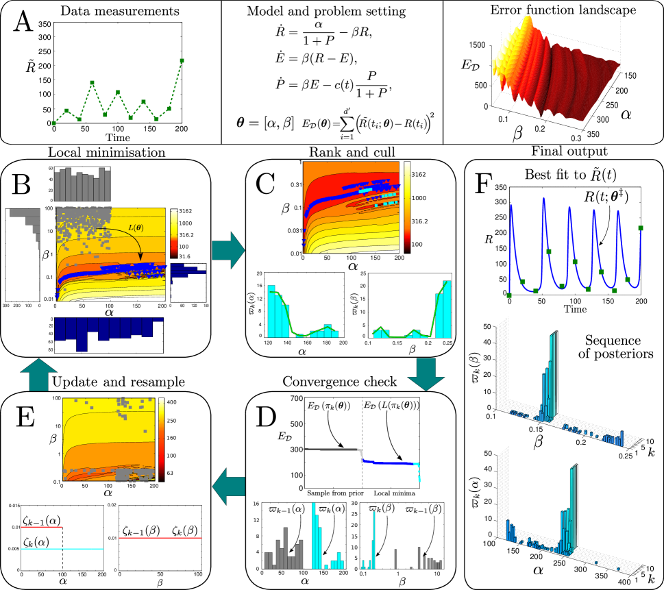
Figure 1: (Colour online) Steps of Algorithm 1 exemplified through the BPM model (10). A: The problem is defined by the data set, the model and the error function to be minimised. Note the rugged landscape of the error function in the parameter plane $(\alpha,\beta)$, with many local minima. B: In the first iteration, we simulate $J$ points in parameter space from the uniform initial prior $\pi_{0}(\boldsymbol{\theta})$ (grey squares, grey histograms) which are then minimised locally with a Nelder-Mead algorithm $L(\boldsymbol{\theta})$ (blue triangles, blue histograms). The local optimisation aligns the parameter sets onto the level curves of $E_{\mathcal{D}}$. C: The $B$ best local minima (top, light blue squares) are selected and considered to be samples from the posterior distribution (bottom, light blue histograms). D: Convergence of the error of the samples (top, local minima in blue, $B$ lowest in light blue) and of the posterior distributions (bottom, light blue) are checked against the errors of the sample (top, in grey) and the priors (bottom, in grey). E: If convergence is not achieved, the historical prior is updated (previous historical prior in red updated to light blue) and a new set of $J$ points are simulated from the posterior with probability $p_{m}$ and from the historical prior with probability $1-p_{m}$ (grey squares). This new sample is fed back to the local minimisation step B . F: The algorithm stops when convergence is reached (after nine iterations, in this case) providing an optimal parameter set $\boldsymbol{\theta}^{\ddagger}$ (top, time course of optimal model in blue) and the sequence of optimised posteriors at each iteration (bottom).

Algorithm 1 Squeeze-and-Breathe optimisation.

  Set running parameters of algorithm: $B,J\in\mathbb{N}$, $p_{m}\in[0,1]$, Tol

  Choose initial priors $\pi_{0}(\boldsymbol{\theta})$ and $\zeta_{0}(\boldsymbol{\theta})$.

  Set $\mathcal{H}_{0}=\emptyset$ and $k\leftarrow 1$.

  repeat

     Let $\mathcal{H}_{k}=\mathcal{H}_{k-1}$.

     Simulate $J$ points from $\pi_{k-1}(\boldsymbol{\theta})$ through re-population.

     for $\ell=1\to J$ do

        Obtain local minimum $\boldsymbol{\theta}_{\ell}^{*}=L(\boldsymbol{\theta}_{\ell})$.

        Store the pair $[\boldsymbol{\theta}_{\ell}^{*},E_{\mathcal{D}}(\boldsymbol{\theta}_{\ell}^{*})]$ in $\mathcal{H}_{k}$.

     end for

     Rank and cull the set of local minima: $\mathcal{H}_{k}=\mathcal{RC}_{B}\left(\mathcal{H}_{k}\right)$

     Define the posterior $\varpi_{k}(\boldsymbol{\theta})$ from the sample $\mathcal{H}_{k}$.

     Update $\zeta_{k}(\boldsymbol{\theta})$ from $\zeta_{k-1}(\boldsymbol{\theta})$ and $\varpi_{k}(\boldsymbol{\theta})$.

     Update the prior $\pi_{k}(\boldsymbol{\theta})\sim p_{m}\varpi_{k}(\boldsymbol{\theta})+(1-p_{m})\zeta_{k}(\boldsymbol{\theta})$.

     $k\leftarrow k+1$.

  until $\phi_{k}<Tol$ and $\mathcal{MW}\left(\varpi_{k}(\boldsymbol{\theta}),\varpi_{k-1}(\boldsymbol{\theta})\right)=0$

Algorithm 1 presents the pseudo-code for our method using the definitions above. The iterations produce progressively more refined distributions of the parameter vector. At each iteration $k$, a population simulated from the prior distribution $\pi_{k-1}(\boldsymbol{\theta})$ is locally minimised followed by ranking and culling of the local minima to create a posterior distribution $\varpi_{k}(\boldsymbol{\theta})$ (squeeze step). This distribution is then combined with an encompassing historical prior to generate the updated prior $\pi_{k}(\boldsymbol{\theta})$ (breathe step). The iteration loop terminates when the difference between the mean errors of consecutive posteriors is smaller than the tolerance and the samples of the posteriors are indistinguishable. We now explain these steps in detail (Fig. 1) through the BPM model (see Sec. 3.1).

1. Formulation of the optimisation: The data set $\mathcal{D}$ and the model equations parameterised by $\boldsymbol{\theta}$ allow us to define an error function $E_{\mathcal{D}}(\boldsymbol{\theta})$ whose global minimum corresponds to the best model.

   In our illustrative example, the BPM model (10) has the parameter vector $\boldsymbol{\theta}=[\alpha,\beta]$ and the error function is depicted in Fig. 1A. The global optimisation on the rugged landscape of this function is computationally hard.

2. Initialisation:

   • Set the running parameters of the algorithm: the size of the simulated population, $J$; the size of the surviving population after culling, $B$; the update probability, $p_{m}$; and the tolerance, $Tol$.

     In this example, $J=500$, $B=50$, $p_{m}=0.95$ and $Tol=10^{-5}$.

   • Choose $\pi_{0}(\boldsymbol{\theta})$, the initial prior distribution of the parameter vector.

     In this case, we take $\alpha$ and $\beta$ to be independent and uniformly distributed: $\pi_{0}(\boldsymbol{\theta})\sim U(0,100)\times U(0,100)$.

   • Initialise $\zeta_{0}(\boldsymbol{\theta})=\pi_{0}(\boldsymbol{\theta})$, the historical prior of the parameters.

   • Simulate $J$ points from $\pi_{0}(\boldsymbol{\theta})$ to generate the initial sample $\{\widehat{\boldsymbol{\theta}}_{0}\}_{1}^{J}$.

3. Iteration (step $k$): Repeated until termination criterion is satisfied. Figure 1 shows the first iteration of our method applied to the BPM example.

   1. Local minimisation: Apply local minimisation to the simulated parameters from the ’prior’ $\{\widehat{\boldsymbol{\theta}}_{k-1}\}_{1}^{J}$ and map them onto local minima of $E_{\mathcal{D}}(\boldsymbol{\theta})$ to generate $\{L(\widehat{\boldsymbol{\theta}}_{k-1})\}_{1}^{J}\in\mathbb{M}$.

      Here we use the Nelder-Mead simplex method (Nelder and Mead, 1965), though others can be used. Figure 1B shows the simulated points from $\pi_{0}(\boldsymbol{\theta})$ (grey squares) and its corresponding histograms (in grey). After local minimisation, this sample is mapped onto the dark blue triangles in Fig. 1B (histograms in dark blue). Note how the local minima align with the level curves of $E_{\mathcal{D}}$ with a markedly different distribution to the uniform prior. Note also that many of the optimised values of $\alpha$ lie outside the range of the prior $(0,100)$ and are now distributed over the interval $(0,200)$. On the other hand, the values of $\beta$ have collapsed inside $(0,1)$.

   2. Ranking and culling: Rank the $J+B$ local minima from the $k-1$ and $k$ iterations, select the $B$ points with the lowest $E_{\mathcal{D}}$ and cull (discard) the rest:

      $$\mathcal{RC}_{B}\left(\{L(\widehat{\boldsymbol{\theta}}_{k-1})\}_{1}^{J}\cup\{\widehat{\boldsymbol{\theta}}_{k-1}^{\dagger}\}_{1}^{B}\right)=\{\widehat{\boldsymbol{\theta}}_{k}^{\dagger}\}_{1}^{B}.$$

      Denote the best parameter vector of this set as $\boldsymbol{\theta}_{k}^{\ddagger}=\underset{E_{\mathcal{D}}}{\min}\left(\{\widehat{\boldsymbol{\theta}}_{k}^{\dagger}\}_{1}^{B}\right)$. We consider $\{\widehat{\boldsymbol{\theta}}_{k}^{\dagger}\}_{1}^{B}$ to be a sample from the optimised (‘posterior’) distribution, $\varpi_{k}(\boldsymbol{\theta})$.

      The $B=50$ best parameter sets are shown (light blue squares) in Fig. 1C (light blue histograms).

   3. Termination criterion: Check that the difference between the mean errors of the consecutive optimised samples is smaller than the tolerance: $\phi_{k}\leq Tol$. We also gauge the ‘convergence’ of the posteriors through the Mann-Whitney (MW) test to determine if the samples from consecutive posteriors are distinguishable:

      $$\mathcal{MW}(\varpi_{k-1}(\boldsymbol{\theta}),\varpi_{k}(\boldsymbol{\theta}))\equiv\mathcal{MW}\left(\{\widehat{\boldsymbol{\theta}}_{k-1}^{\dagger}\}_{1}^{B},\{\widehat{\boldsymbol{\theta}}_{k}^{\dagger}\}_{1}^{B}\right),$$

      where $\mathcal{MW}$ is a $0$-$1$ flag. The MW test gives additional information about the change of the optimised posteriors from one iteration to the next.

      Figure 1D shows the convergence check for the first iteration of the BPM model: (i) top, errors of the sampled prior (grey, left) with errors of the local minima (dark blue, right) and the $B$ surviving points (light blue); (ii) bottom, histograms of the prior (grey) and the posterior (light blue). Clearly, in this iteration neither the error nor the distributions have converged so the algorithm does not stop.

   4. Update of historical prior and generation of new sample: If convergence is not achieved, update the historical prior $\zeta_{k}(\boldsymbol{\theta})$ as a uniform distribution over the union of the supports of the existing historical prior and the calculated posterior (6). Equivalently, the support of the historical prior extends over the union of the sequence of all historical priors $\{\zeta_{0}(\boldsymbol{\theta}),\ldots,\zeta_{k-1}(\boldsymbol{\theta})\}$ and of all posteriors $\{\varpi_{1}(\boldsymbol{\theta}),\ldots,\varpi_{k}(\boldsymbol{\theta})\}$.

      As shown in Fig. 1E for the BPM example, the marginal of the historical prior for $\alpha$ is expanded to $U(0,200)$, since the optimised parameter sets have reached values as high as 200. Meanwhile, the $\beta$ marginal of the historical prior remains unchanged as $U(0,100)$ because there has been no expansion of the support.

      The historical prior is used to mutate the updated prior before the next iteration by constructing a weighted mixture of the posterior and the historical prior with weight $p_{m}$, as shown in (7). We re-populate from this updated prior by simulating from the posterior with probability $p_{m}=0.95$ and from the historical prior with probability $(1-p_{m})$ to generate the new sample $\{\widehat{\boldsymbol{\theta}}_{k}\}_{1}^{J}$ and iterate back.

      Figure 1E shows the sample of $J$ points simulated from the new prior. The $\alpha$-components of most points are between 100 and 200 and the $\beta$-components are between 0.1 and 1.0, but there are a few that lie outside the support of the posterior. The process in panels B. C, D, and E of Fig. 1 is iterated for this new set of points.

4. Output of the algorithm: When the convergence criteria have been met, the iteration stops at iteration $k^{*}$ and the last $\boldsymbol{\theta}_{k^{*}}^{\ddagger}$ is presented as the optimal parameter set for the model. We can also examine the sequence of optimised parameter distributions $\{\varpi_{1}(\boldsymbol{\theta}),\ldots,\varpi_{k^{*}}(\boldsymbol{\theta})\}$ obtained for all iterations (Fig. 1F).

3 Application to biological examples

We apply our algorithm to three biological examples of interest. The first two correspond to simulated data from models in the literature, while in the third example we apply our algorithm to unpublished experimental data of the dynamical response of an inducible genetic promoter constructed for an application in Synthetic Biology.

3.1 BPM model of gene-product regulation

	Min.			Conv.	Conv.
$k$	Error	$\alpha_{k}^{\ddagger}$	$\beta_{k}^{\ddagger}$	$\varpi_{k}(\alpha)$	$\varpi_{k}(\beta)$	$\phi_{k}$
1	56.0941	193.7447	0.1304	-	-	-
2	28.2735	246.7510	0.1528	No	No	133.9020
3	27.2083	248.7557	0.1532	No	No	6.8542
4	26.9838	250.3593	0.1536	No	No	0.6532
5	26.6504	251.7189	0.1538	No	No	0.3281
6	26.6504	251.7189	0.1538	No	No	0.1963
7	26.6504	251.7189	0.1538	Yes	Yes	0.0118
8	26.6504	251.7189	0.1538	No	No	0.0131
9	26.6504	251.7189	0.1538	Yes	Yes	$1.414\times 10^{-6}$

Table 1: Results of the fitting of the BPM model with Algorithm 1: smallest error of iteration $k$; the best values $\alpha_{k}^{\ddagger}$ and $\beta_{k}^{\ddagger}$; whether the distributions have converged; and the difference of the mean errors of the optimised population.

The Bliss-Painter-Marr (BPM) model (Bliss et al., 1982) describes the behaviour of a gene-enzyme-product control unit with a negative feedback loop:

$$\dot{R} =\frac{\alpha}{1+P}-\beta R,$$

$$\dot{E} =\beta(R-E),$$ (10)

$$\dot{P} =\beta E-c(t)\frac{P}{1+P}.$$

Here, $R,E$ and $P$ are the concentrations (in arbitrary units) of mRNA, enzyme and product, respectively. The degradation rate of the product has an explicit time dependence, which in this case has the form of a ramp saturation:

$$c(t)=\left\{\begin{array}[]{cl}5+0.2t&0\leq t<50,\\ 15&t\geq 50.\end{array}\right.$$

The model represents a gene that codes for an enzyme which in turn catalyses a product that inhibits the transcription of the gene. This self-inhibition can lead to oscillations, which have been shown to occur in the tryptophan operon in E. coli (Bliss et al., 1982).

We construct a data set from simulations of this model with $\boldsymbol{\theta}_{\mathrm{real}}=[\alpha,\beta]=[240,0.15]$ and initial conditions $R(0)=E(0)=P(0)=0$. The data set $\mathcal{D}$ consists of 10 measurements of $R(t)$ at particular times with added gaussian noise drawn from $\mathcal{N}(0,15^{2})$ (Table 3). The error function $E_{\mathcal{D}}(\boldsymbol{\theta})$ (4) corresponds to a non-convex optimisation landscape: a complex rugged surface with many local minima making global optimisation hard (Fig. 1A).

We use Algorithm 1 to estimate the ‘unknown’ parameter values from the ‘measurements’ of $R$, as illustrated in Sec. 2.3 and Fig. 1. Feigning ignorance of the true values, we choose a uniform prior distribution with range $[0,100]$ for both parameters: $\pi_{0}(\boldsymbol{\theta})\sim[U(0,100),U(0,100)]$. The rest of the paramters are set to: $J=500$, $B=50$, $p_{m}=0.95$ and $Tol=10^{-5}$. Note that the true value of $\alpha$ falls outside of the assumed range of our initial prior, while the range of $\beta$ in our initial prior is two orders of magnitude larger than its true value. This level of uncertainty about parameter values is typical in data fitting for biological models.

Figure 1 highlights a key aspect of our algorithm: the local minimisation can lead to local minima outside of the range of the initial prior. Furthermore, our definition of the historical prior ensures that successive iterations can find solutions within the largest hypercube of optimised solutions in parameter space. In this example, the algorithm moves away from the $U(0,100)$ prior for $\alpha$ and finds a distribution around 240 (the true value) after three iterations, while in the case of $\beta$, the distribution collapses to values around 0.15 after one iteration. Although the algorithm finds the minimum $\boldsymbol{\theta}^{\ddagger}$ after 5 iterations, the algorithm is terminated after 9 iterations, when the posterior distributions are similar (according to the MW test) and the mean errors have also converged (Table 1). The estimated parameters for this noisy data set are $\boldsymbol{\theta}_{k^{*}}^{\ddagger}=[251.7189,0.1530]$. In fact, the error of the estimated parameter set is lower than that of the real parameters: $E_{\mathcal{D}}(\boldsymbol{\theta}^{\ddagger})=26.65<E_{\mathcal{D}}(\boldsymbol{\theta}_{\mathrm{real}})=28.26$, due to the noise introduced in the data. When a data set without noise is used, the algorithm finds the true value of the parameters to 9 significant digits (not shown).

3.2 SIR epidemics model

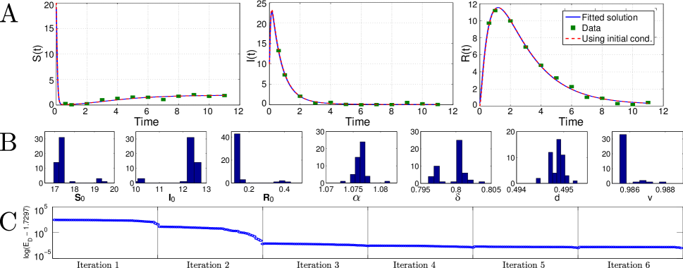
Figure 2: (Colour online) A: Time courses of the SIR model (11). Green squares are simulated ‘data’ points (Table 4) and bold blue lines are the model fit with the best parameters $\alpha^{\ddagger}=1.0726$, $\gamma^{\ddagger}=0.7964$, $d^{\ddagger}=0.4945$, and $v^{\ddagger}=0.9863$ and the best fit initial conditions $S_{0}^{\ddagger}=19.1591$, $I_{0}^{\ddagger}=10.3016$, and $R_{0}^{\ddagger}=0.3861$. Red dashed lines use the best fit parameters and the real initial conditions. The minimum error is $E_{\mathcal{D}}(\boldsymbol{\theta}^{\ddagger})=1.7297$. B: Histogram of the values of the 50 best parameters and initial conditions of the model obtained after convergence at six iterations. C: Convergence of the error of the optimised samples at every iteration relative to the final error.

Susceptible-Infected-Recovered (SIR) models are widely used in epidemiology to describe the evolution of an infection in a population (Anderson and May, 1992). In its simplest form, the SIR model has three variables: the susceptible population $S$, the infected population $I$ and the recovered population $R$:

$$\dot{S} =\alpha-(\gamma I+d)S,$$

$$\dot{I} =(\gamma S-v-d)I,$$ (11)

$$\dot{R} =vI-dR.$$

The first equation describes the change in the susceptible population, growing with birth rate $\alpha$ and decreasing by the rate of infection $\gamma IS$ and the rate of death $dS$. The infected population grows by the rate of infection $\gamma IS$ and decreases by the rate of recovery $vI$ and the rate of death $dI$. The recovered population grows by the rate of recovery $vI$ and decreases by the death rate $dR$. Here we use the same form of the equations as Toni et al. (2009).

The data generated from the model (11) (see Table 4) was obtained directly from Toni et al. (2009). Hence the original parameter values were not known to us and further we assumed the initial conditions also to be unknown and fitted them as parameters. We used Algorithm 1 to estimate $\alpha$, $\gamma$, $v$, and $d$ and initial conditions $S_{0}$, $I_{0}$, and $R_{0}$. The prior marginal distributions for all parameters were set as $U(0,100)$. The other parameters were set to: $J=1000$, $B=50$, $p_{m}=0.95$ and $Tol=10^{-5}$. The algorithm converged after six iterations. Figure 2A shows the prediction of the model (11) with the best parameters estimated by our algorithm. The fit is good with little difference between the curves obtained using the real initial conditions and the ones estimated by our method.

The posterior distributions after six iterations of the algorithm are shown on Fig. 2B. The errors obtained after each local minimisation in a decreasing order on each iteration are shown on a semilogarithmic scale in Fig. 2C. We can observe how the errors decrease several orders of magnitude over the first three iterations and converge steadily during the last three iterations until $\phi_{k}\leq Tol$.

3.3 An inducible genetic switch from Synthetic Biology

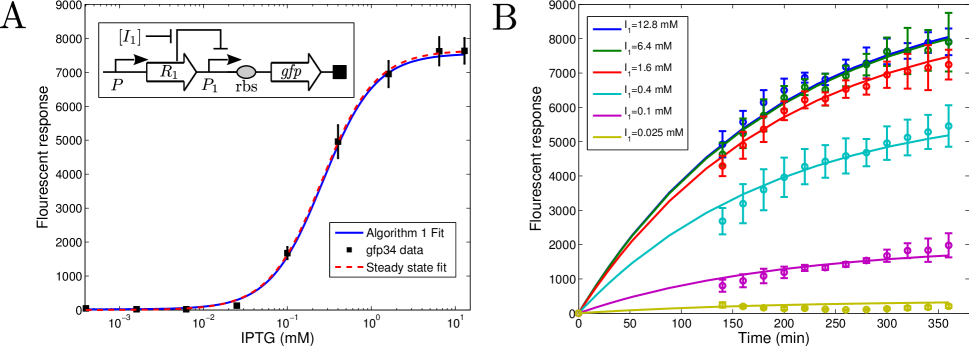
Figure 3: A: (Colour online) Inset: An inducible genetic switch consisting of $P_{1}$, a negatively regulated environment-responsive promoter. The repressor R₁ promoted by $P$ regulates $P_{1}$. The switch is responsive to an exogenous inducer $I_{1}$, which binds to R₁ to relieve its repression on $P_{1}$ and to turn on the transcription of the downstream target gene, such as a gfp. The ribosome binding site (rbs) is used to tune the translation efficiency of the downstream gene. Plot: Fluorescent response of the switch with gfp-34 to different doses of IPTG (circles). Stationary solutions of Eq. (12) using the parameters obtained with Algorithm 1 (solid lines). B: Time course of the fluorescent response of the switch with gfp-34 to several doses of IPTG (circles) and time-dependent solutions of Eq. (12) using the parameters obtained with Algorithm 1 (solid lines). Similarly good fits were obtained for responses to $I_{1}$ = 0.0063, 0.0016, 0.0004, and 0.0 mM (not shown).

The use of inducible genetic switches is widespread in synthetic biology and bioengineering as building blocks for more complicated gene circuit architectures. An example is shown schematically in the inset of Fig. 3A. This environment-responsive switch is used to control the expression of a target gene $G$ (usually tagged with green fluorescent protein or gfp) through the addition of an exogenous small molecule $I_{1}$ (e.g., isopropyl thiogalactopyranoside or IPTG). The input-output behaviour of this system can be described by the following ordinary differential equation (Szallasi et al., 2006; Alon, 2007):

$$\dot{G}=\alpha k_{1}+\frac{k_{1}I_{1}^{n_{1}}}{K_{1}^{n_{1}}+I_{1}^{n_{1}}}-dG.$$ (12)

Here, $\alpha k_{1}$ is the basal activity of the promoter $P_{1}$ and $dG$ is the linear degradation term. The second term is a Hill function that models the cooperative transcription activation in response to the inducer $I_{1}$ with maximum expression rate $k_{1}$, constant $K_{1}$ and Hill coefficient $n_{1}$.

The $lacI$–$P_{lac}$ switch has been characterised experimentally in response to different doses of IPTG in Wang (2010); Wang et al. (2011). Equation (12) can be solved explicitly and one can use nonlinear least squares and the analytical solution to fit data at stationarity (i.e., at long times) and estimate $\alpha$, $n_{1}$, $K_{1}$, and the ratio $k_{1}/d$. These estimates have been obtained assuming equilibrium ($\dot{G}=0$) and initial condition $G(0)=0$ by Wang et al. (2011) (Table 2).

In fact, the experiments measured time series of the expression of $G$ every 20 minutes from $t=140$ to $360$ min. for different doses of inducer $I_{1}=0.0,3.9\times 10^{-4},1.6\times 10^{-3},6.3\times 10^{-3},2.5\times 10^{-2},0.1,0.4,1.6,6.4,12.8$ mM, with two different reporters (gfp-30 and gfp-34). See Tables 5 and 6 Instead of assuming equilibrium and using only the data for $t>300$ min as done previously (Wang et al., 2011), we apply Algorithm 1 to all the data with the full dynamical equation (12) to estimate $\boldsymbol{\theta}=[\alpha,k_{1},n_{1},K_{1},d]$. In this case, we used initial priors $U(0,1)$ for $\alpha$ and $n_{1}$; and $U(0,20)$ for $k_{1}$, $K_{1}$ and $d$. The other parameters were set to: $J=1000$, $B=50$, $p_{m}=0.95$, and $Tol=10^{-5}$.

Our algorithm converged after five iterations to the parameter values in Table 2. The parameter estimates provide good fits to both the time courses (Fig. 3B) and to the dose response data (Fig. 3A). The values of $K_{1}^{\ddagger}$ and $n_{1}^{\ddagger}$ obtained here are similar those obtained in Wang (2010) by using only stationary data. This is reassuring since these parameters are related to the dose threshold to half maximal response and to the steepness of the sigmoidal response, both static properties. On the other hand, the values of $\alpha$ and the ratio $k_{1}/d$ differ to some extent due to the (imperfect) assumption in Wang (2010) that steady state had been reached at $t=300$ min. As Fig. 3B shows, $G$ is not at steady state then. Hence the parameter values obtained with our method should give a more faithful representation of the true dynamical response of the switch.

	Wang (2010)		Algorithm 1
Parameter	gfp-30	gfp-34	gfp-30	gfp-34
$\alpha^{\ddagger}$	$0.0012\pm 0.027$	$1.4720\times 10^{-9}$	0.0043	0.0024
$k_{1}^{\ddagger}$	N/A	N/A	76.1354	63.6650
$n_{1}^{\ddagger}$	$1.3700\pm 0.270$	$1.3690\pm 0.021$	1.4832	1.3879
$K_{1}^{\ddagger}$	$0.2280\pm 0.039$	$0.2590\pm 0.021$	0.2467	0.2641
$d^{\ddagger}$	N/A	N/A	0.0069	0.0052
$k_{1}^{\ddagger}/d^{\ddagger}$	$9456\pm 487$	$7648\pm 152$	10983.34	12163.04

Table 2: Parameter values obtained from gfp-30 and gfp-34 data. In Wang (2010), only the steady state solution was used. Hence only the ratio of $k_{1}$ and $d$ can be estimated.

4 Discussion

In this work, we have presented an optimisation algorithm that brings together ingredients from Evolutionary Algorithms, local optimisation and Sequential Monte Carlo. The method is particularly useful for determining parameters of ordinary differential equation models from data. Our approach can also be used in other contexts where an optimisation problem has to be solved on complex landscapes, or when the objective function cannot be written explicitly. The algorithm proceeds by generating a population of solutions through Monte Carlo sampling from a prior distribution and refining those solutions through a combination of local optimisation and culling. A new prior is then created as a mixture of a historical prior (which records the broadest possible range of solutions found) and the distribution of the optimised population. This iterative process combines a strong concentration of the Monte Carlo sampling through local optimisation with the possibility that solutions can be found outside of the initial prior.

We have illustrated the application of the algorithm to ODE models of biological interest and have found it to perform efficiently. The algorithm also works well when applied to larger problems with tens of parameters in a signal transduction model (paper in preparation). The efficiency of the algorithm hinges on selecting appropriate running parameters. For instance, the number of samples from the prior $J$ should be large enough to allow for significant sampling of the parameter space while small enough to limit the computational cost. We have found that simulating $J=350-500$ points in models of up to 10 parameters and keeping the best 15% of the local minima leads to termination within fewer than 20 iterations. In our implementation, the Nelder-Mead minimisation is capped at 300 evaluations. These guidelines would result in  150,000 evaluations of the objective function per iteration. Therefore our method can become computationally costly if the objective function is expensive to evaluate, e.g. in stiff models that are difficult to solve numerically. In essence, our algorithm proposes a trade-off: fewer but more costly iterations. It is important to remark that, as with any other optimisation heuristic for non convex problems, there are no strict guarantees of convergence to the global minimum. Therefore, it is always advisable to run the method with different starting points and different settings to check for consistency of the solutions obtained.

The generation of iterative samples of the parameters draws inspiration from Monte Carlo methods (Sisson et al., 2007; Toni and Stumpf, 2009; Toni et al., 2009) but without pursuing the strict guarantees that the nested structure of the distributions in ABC-SMC provides. Our evolutionary approach adopts a highly focused Monte Carlo sampling driven by a sharp local search with culling. Hence our iterative procedure generates samples that only reflect properties of the set of local minima (up to numerical cutoffs) without any focus on the global convergence of the distributions. As noted by Toni et al. (2009), the distributions of the parameters (both their sequence and the final distributions) give information about the sensitivity of the parameters: parameters with narrow support will be more sensitive than those with wider support. Future developments of the method will focus on establishing a suitable theoretical framework that facilitates its use in model selection. Other work will consider the possibility of incorporating a stochastic ranking strategy in the selection of solutions, similar to that present in the SRES algorithm (Runarsson and Yao, 2000), in order to solve more general optimisation problems with complex feasible regions.

Appendix A BPM model data

t	R
0	0
20	43.5373
40	13.3667
60	140.8903
80	29.2816
100	108.1722
120	19.0093
140	75.0065
160	14.4018
180	50.4473
200	217.1082

Table 3: BPM data.

Table 3 shows data obtained from a simulation of the BPM model from equations (6) using parameters $\alpha=240$ and $\beta=0.15$, initial conditions $R(0)=0$, $E(0)=0$, $P(0)=0$, and adding random noise sampled from a $N(0,15^{2})$ distribution. Only the data for variable $R$ was obtained.

Appendix B SIR model data

t	S	I	R
0.6	0.12	13.17	9.42
1.0	0.12	7.17	11.19
2.0	0.10	2.36	10.04
3.0	0.38	0.92	6.87
4.0	1.00	0.62	4.45
5.0	1.20	0.17	3.01
6.0	1.46	0.28	1.76
7.0	1.38	0.10	1.29
8.0	1.57	0.03	0.82
9.0	1.46	0.29	0.52
10.0	1.25	0.10	0.23
11.0	1.56	0.22	0.20

Table 4: SIR data.

Table 4 shows data for the SIR model generated from equations (8) using initial conditions $S(0)=20$, $I(0)=10$, and $R(0)=0$ with added random noise sampled from a $N(0,0.2^{2})$ distribution as appears in Ref. Toni et al. (2009).

Appendix C Genetic switch data

Tables 5 and 6 show the fluorescent response of IPTG-induced genetic switches described in Ref. Wang (2010) and Wang et al. (2011).

t	0mM	0.0004mM	0.0016mM	0.0063mM	0.025mM	0.1mM	0.4mM	1.6mM	6.4mM	12.8mM
0	0	0	0	0	0	0	0	0	0	0
140	88.6	177.8	174.4	197.8	210.4	1043.6	3945.8	5971	6643.8	6521.8
160	120.2	156.4	160.6	165.6	209.8	1300.8	4695.2	6768.4	7361.8	7513.8
180	66.6	96.4	94.6	126.4	171.6	1438.4	5238.8	7465.2	7801	8002.4
200	42.8	72.2	76.2	88	134.2	1578	5658	7914	8458	8542.8
220	37	64.8	61.2	55	135.8	1667	5799.6	8380.2	8976	8914.8
240	39.6	56.6	60.4	65.8	142.8	1758.6	6108.6	8601.4	9172.6	8957
260	36.2	47.6	62	69.8	143.6	1859.8	6104	9041.8	9528.6	9252.8
280	50.8	55.6	58.2	74.2	170.6	1968.2	6554.4	9071.6	9449	9018.4
300	39.6	51	40.8	60.2	197.8	2143.4	6452.2	8396.2	9269.2	9261.2
320	50.4	62.8	65.6	82	273.6	2317.8	6880.8	8941.2	9887.6	9982.8
340	53.8	71.4	71	88.6	296	2512.8	7052.2	8972.8	9694.6	10108
360	45.6	66	61.6	69.2	340.8	2639.2	7047.8	9103.6	9911	10018.4

t	0mM	0.0004mM	0.0016mM	0.0063mM	0.025mM	0.1mM	0.4mM	1.6mM	6.4mM	12.8mM
0	0	0	0	0	0	0	0	0	0	0
140	215	163.4	124.8	134	119	230.4	721.2	1001.8	1095.8	701
160	141.6	116.6	95.4	86	40	320.6	937	1112.2	1054	903.2
180	131.6	112.2	117.6	84	81	252.2	825.2	727.4	1026.8	679.2
200	69.8	42.4	37.8	39	44.2	225.2	688.4	829.8	761.6	584.6
220	55	58.4	59	60.6	50.4	169.2	645.8	713.6	739.6	454
240	38.8	48	30.8	43.4	42.2	148.8	366	418.6	453.8	668.2
260	42.2	44	48.6	41	53.8	152.8	496.4	638.4	547.8	626.2
280	55.2	54.4	51.8	53.6	76	257.2	498.2	722.2	889.8	606.2
300	50.4	57.4	62	67.8	95	339.8	447.4	835.6	693.2	602.6
320	52.6	69.6	78.4	81.2	146.8	385.8	540.4	776.4	1084.2	580
340	57	60.6	73.8	65.6	144.6	401.2	466.4	396.6	560.4	702
360	61.6	73.2	77.2	68.6	151	400	374.8	251	742	436.2

Table 5: gfp30 fluorescence measurements (top) and standard deviations (bottom).

t	0mM	0.0004mM	0.0016mM	0.0063mM	0.025mM	0.1mM	0.4mM	1.6mM	6.4mM	12.8mM
0	0	0	0	0	0	0	0	0	0	0
140	149.1	199.7	107.4	124.6	242.4	801.9	2682.7	4292.3	4633.3	4923.8
160	96	212.2	121.6	78.4	199.3	945	3192.9	4893.7	5243.3	5572.6
180	64.3	178.7	73.7	40.4	158.7	1083.8	3598.4	5362.7	5762.6	6139.4
200	32.2	92.5	43.2	43.7	135.1	1190.5	3961.4	5901.6	6282.9	6499.9
220	56.4	86.5	51.5	43.5	142.8	1320.4	4274.4	6218.6	6589.5	6866.5
240	42.4	54.6	16.5	23.9	116.3	1330.6	4424.9	6247.9	6514.3	6815.1
260	31	49.9	11.3	13.4	100.4	1422.8	4583.5	6531	6917.5	7177.6
280	34.7	55.5	13	16.4	107.1	1535.8	4680.4	6609.6	7247.2	7290.1
300	33.2	46.1	21.7	22.1	129.7	1675.5	4958.5	6949.3	7620.3	7631.3
320	29.5	39	8.7	22.5	154	1824.5	5122.3	7053.4	7642.7	7645.1
340	31.2	43.2	19.1	27.1	172.2	1836.2	5282.7	7156.9	7661.2	7889.3
360	28	40	10.9	28.9	202.4	1979.3	5456.4	7245.6	7899.1	7910.6

t	0mM	0.0004mM	0.0016mM	0.0063mM	0.025mM	0.1mM	0.4mM	1.6mM	6.4mM	12.8mM
0	0	0	0	0	0	0	0	0	0	0
140	89.4	85.8	209.2	120.8	77.8	175.8	383.6	295.4	332.6	382
160	59.4	23	166.4	111.6	40.6	188.8	572.2	391.6	430.6	326.2
180	31.6	38.6	135.4	51.2	24.8	210.6	597	370.8	467.6	363.8
200	45.2	60.4	83.2	65.2	42	166	573.2	273.6	341.6	337
220	14	27.4	90.2	51.2	25	90	513.8	249.6	234	145.2
240	25.2	32.2	53.8	30.6	16.2	70	475.2	187.6	464.8	168
260	14.8	17.2	47.4	23.8	14.2	68.8	511.8	256	300.6	214
280	20	15.4	46.6	16.6	15.8	70.6	395.8	237.6	313.6	454.6
300	17.8	17.8	37.8	29.8	29.2	178.2	486.6	383.8	416.2	377.2
320	21	21.2	43	26.4	46.8	216.2	519.6	507.4	674.8	227
340	26	22.2	36.8	25.4	46.6	340.8	495.6	655.6	594.2	299.4
360	15.2	13	38.4	8.6	50	350.4	604.8	434.2	853.8	387.8

Table 6: gfp34 fluorescence measurements (top) and standard deviations (bottom).

References

- Alon (2007) Alon, U. (2007). An introduction to systems biology: design principles of biological circuits. Chapman and Hall/CRC mathematical & computational biology series. Chapman & Hall/CRC.
- Anderson and May (1992) Anderson, R. M. and May, R. M. (1992). Infectious Diseases of Humans Dynamics and Control. Oxford University Press.
- Bliss et al. (1982) Bliss, R. D., Painter, P. R., and Marr, A. G. (1982). Role of feedback inhibition in stabilizing the classical operon. Journal of Theoretical Biology, 97(2), 177 – 193.
- Brewer et al. (2008) Brewer, D., Barenco, M., Callard, R., Hubank, M., and Stark, J. (2008). Fitting ordinary differential equations to short time course data. Philosophical Transactions of the Royal Society A: Mathematical, Physical and Engineering Sciences, 366(1865), 519–544.
- Brown and Sethna (2003) Brown, K. S. and Sethna, J. P. (2003). Statistical mechanical approaches to models with many poorly known parameters. Physical Review E, 68(2), 021904.
- Chen et al. (2010) Chen, W. W., Niepel, M., and Sorger, P. K. (2010). Classic and contemporary approaches to modeling biochemical reactions. Genes Dev, 24(17), 1861–1875.
- Edelstein-Keshet (1988) Edelstein-Keshet, L. (1988). Mathematical models in biology. Classics in applied mathematics. SIAM.
- Gershenfeld (1999) Gershenfeld, N. (1999). The nature of mathematical modeling. Cambridge University Press.
- Gutenkunst et al. (2007) Gutenkunst, R. N., Waterfall, J. J., Casey, F. P., Brown, K. S., Myers, C. R., and Sethna, J. P. (2007). Universally Sloppy Parameter Sensitivities in Systems Biology Models. PLoS Comput Biol, 3(10), e189.
- Kirkpatrick et al. (1983) Kirkpatrick, S., Gelatt, C. D., and Vecchi, M. P. (1983). Optimization by simulated annealing. Science, 220(4598), 671–680.
- Lawson and Hanson (1995) Lawson, C. and Hanson, R. (1995). Solving least squares problems. Classics in applied mathematics. SIAM.
- Mitchell (1997) Mitchell, T. M. (1997). Machine Learning. McGraw-Hill, New York.
- Moles et al. (2003) Moles, C. G., Mendes, P., and Banga, J. R. (2003). Parameter Estimation in Biochemical Pathways: A Comparison of Global Optimization Methods. Genome Research, 13(11), 2467–2474.
- Nelder and Mead (1965) Nelder, J. A. and Mead, R. (1965). A Simplex Method for Function Minimization. The Computer Journal, 7(4), 308–313.
- Papachristodoulou and Recht (2007) Papachristodoulou, A. and Recht, B. (2007). Determining Interconnections in Chemical Reaction Networks. In American Control Conference, 2007., pages 4872–4877.
- Powell (1998) Powell, M. J. D. (1998). Direct Search Algorithms for Optimization Calculations. Acta Numerica, 7(-1), 287–336.
- Runarsson and Yao (2000) Runarsson, T. and Yao, X. (2000). Stochastic ranking for constrained evolutionary optimization. IEEE Transactions on Evolutionary Computation, 4(3), 284 –294.
- Schwefel (1995) Schwefel, H. (1995). Evolution and optimum seeking. Sixth-generation computer technology series. Wiley.
- Sisson et al. (2007) Sisson, S. A., Fan, Y., and Tanaka, M. M. (2007). Sequential Monte Carlo without likelihoods. Proc Natl Acad Sci USA, 104(6), 1760–1765.
- Sontag (2002) Sontag, E. (2002). For Differential Equations with r Parameters, 2r+1 Experiments Are Enough for Identification. Journal of Nonlinear Science, 12, 553–583.
- Strogatz (1994) Strogatz, S. H. (1994). Nonlinear Dynamics And Chaos. With Applications to Physics, Biology, Chemistry, and Engineering. Studies in nonlinearity. Perseus Books Group.
- Szallasi et al. (2006) Szallasi, Z., Stelling, J., and Periwal, V. (2006). System modeling in cell biology: from concepts to nuts and bolts. Bradford Book. MIT Press.
- Toni and Stumpf (2009) Toni, T. and Stumpf, M. P. H. (2009). Simulation-based model selection for dynamical systems in systems and population biology. Bioinformatics.
- Toni et al. (2009) Toni, T., Welch, D., Strelkowa, N., Ipsen, A., and Stumpf, M. P. (2009). Approximate Bayesian computation scheme for parameter inference and model selection in dynamical systems. Journal of The Royal Society Interface, 6(31), 187–202.
- Wang (2010) Wang, B. (2010). Design and Functional Assembly of Synthetic Biological Parts and Devices. Ph.D. thesis, Imperial College London.
- Wang et al. (2011) Wang, B., Kitney, R. I., Joly, N., and Buck, M. (2011). Engineering modular and orthogonal genetic logic gates for robust digital-like synthetic biology. Nat Commun, 2, 508.
- Yates et al. (2001) Yates, A., Chan, C. C. W., Callard, R. E., George, A. J. T., and Stark, J. (2001). An approach to modelling in immunology. Brief Bioinform, 2(3), 245–257.
- Zi and Klipp (2006) Zi, Z. and Klipp, E. (2006). SBML-PET: a Systems Biology Markup Language-based parameter estimation tool. Bioinformatics, 22(21), 2704–2705.