Model Inference with Reference Priors

Abstract

We describe the application of model inference based on reference priors to two concrete examples in high energy physics: the determination of the CKM matrix parameters $\bar{\rho}$ and $\bar{\eta}$ and the determination of the parameters $m_{0}$ and $m_{1/2}$ in a simplified version of the CMSSM SUSY model. We show how a 1-dimensional reference posterior can be mapped to the $n$-dimensional ($n$-D) parameter space of the given class of models, under a minimal set of conditions on the $n$-D function. This reference-based function can be used as a prior for the next iteration of inference, using Bayes’ theorem recursively.

1 Introduction

It is typical in high energy physics (HEP) to deal with classes of models, e.g. new physics extensions of the Standard Model (SM), differing by the values of a set of (typically continuous) unknown parameters.

Given a set of experimental measurements, one would like to define the region of the model parameter space that is in agreement with the data. This is what we refer to as Model Inference. The following ingredients are needed:

• a theoretical tool that predicts the expected values of the measured observables, given a point in the model parameter space;

• a multi-dimensional likelihood, built from the available measurements;

• and a statistical procedure that evaluates the level of agreement between the data and the predictions.

While the first and second steps are not controversial, the third step is often polemical and is subject to some degree of arbitrariness. Two main approaches are typically followed: Bayesian, which computes the posterior probability of the expected values of the model parameters given the likelihood and a prior probability, and frequentist, which provides probability statements about possible values of the measurements given the observed data and assumed values of the model parameters.

Historically, most high energy physicists have preferred frequentist statistics because (they say) it allows one to extract statistical information from data without the need for subjective input. In this sense, these physicists are victim of the utopian idea of an analyst-free analysis, in which the “data speak for themselves", independently of the personal opinion and judgement of the physicists who perform the analysis. However, we are rudely awakened from this utopian dream on a daily basis as anybody who has had to evaluate a systematic uncertainty can confirm . Beyond this simple fact, we also tend to underestimate how strongly the subjective beliefs of the analyst enters the earlier stages of an analysis, as for instance when we define the form of the likelihood. Physicists quote results as $m\pm\sigma$, where $m$ and $\sigma$ summarize the result of, perhaps, a likelihood-ratio-based analysis, which already implies assumptions about the form of the likelihood . When estimating the systematic uncertainty, we typically sum the different contributions in quadrature, implying that the systematic errors are uncorrelated and, more importantly, that they may be treated as if they are statistical. This may be true of systematic uncertainties that arise ultimately from other statistics; but many systematic uncertainties are “assigned" based on judgement or official policy.

We push this even further when we perform phenomenological analyses. While connecting the parameters of a model to the experimental observables, we often need to know a set of additional quantities (theoretical nuisance parameters) which are not measurable, but which may be known with some uncertainty through a theoretical calculation. This is the case, for instance, for the non-perturbative QCD parameters determined using lattice QCD calculations. In order to take into account the uncertainty on the predictions correctly, a Bayesian analyst would introduce a prior probability density function (pdf) for the theoretical nuisance parameters based on the best judgement of the theorist. While this is considered dangerously subjective in by many high energy physicists, the same physicists consider it safe to modify the likelihood to take account of the theoretical uncertainty on predictions. This breaks the objective-frequentist-physicists paradigm twice: i) the functional form used to account for theoretical uncertainty is no less subjective than the prior of a Bayesian analysis and ii) the likelihood loses its deep and precise meaning of that function obtained by inserting the observations into the probability density function describing possible observations. Nobody ever did (and it is likely that nobody ever will) measure the theoretical nuisance parameters — indeed, many such parameters such as the factorization and renormalization scales are pure artifacts of our current reliance on perturbation theory in theoretical calculations. As a matter of fact, a physicist performing data analysis is forced to make assumptions. And there is nothing wrong with that as long as the assumptions are clearly stated. The problems come when the assumptions are hidden in the procedure and not transparent to the people not directly involved in the analysis.

The contrasting attitudes described above can be summarized in terms of the following two perceived problems:

• For some high energy physicists, introducing a prior is unacceptable because it brings subjectivity into science. “The origin of the problem lies in the very first Bayesian assumption, namely that unknown model parameters are to be understood as mathematical objects distributed according to PDFs, which are assumed to be known: the priors. Obviously, the choice of the priors cannot be irrelevant; hence, the Bayesian treatment is doomed to lead to results which depend on the decisions made, necessarily on an unscientific basis, by the authors of a given analysis, for the choice of these extraordinary PDFs.”  [1].

• For some statisticians, a meaningful statistical analysis is not possible in the absence of an analysis procedure that allows one to incorporate a priori knowledge in a coherent way. “The frequentist approach to hypothesis testing does not permit researchers to place probabilities of being correct on the competing hypotheses. This is because of the limitations on mathematical probabilities used by frequentists. For the frequentists, probabilities can only be defined for random variables, and hypotheses are not variables (they are not observables)… This limitation for frequentists is a real drawback because the applied researcher would really like to be able to place a degree of belief on the hypothesis. He or she would like to see how the weight of evidence modifies his/her degree of belief (probability) on the hypothesis being true.” [2].

The use of reference priors [3] is emerging as a concrete way to solve the two problems. While a detailed discussion of the reference priors is beyond the scope of this paper, we highlight here their most appealing properties.

The main concern against the use of a Bayesian analysis in HEP is related to a priori ignorance, more than a priori knowledge. Whenever a priori knowledge is available (e.g. the measurement of the luminosity, which is used to translate an observed signal yield into a cross section measurement), there is a general consensus that an evidence-based prior should be used. The real issue is how we should parameterize "ignorance". The use of a flat prior, a HEP standard, is not quite the right answer. Reference priors can be seen as a model of ignorance in the sense that, on average, they maximize the influence of the likelihood relative to the prior; hence they are a solution to this problem. More precisely, for a given likelihood, the reference prior is the prior function that on average maximizes the asymptotic Kullback-Leibler divergence [4] between the prior and the posterior, hence enhancing the role of the likelihood (the data) over the prior. This is exactly the kind of behavior that we would like for a model of ignorance. And this is what we assume the flat prior does for us, when we use it. Unfortunately, the flatness of the prior is not invariant under reparameterization. Unlike the flat prior, reference priors give reparameterization-invariant results in the cases typically considered in HEP (e.g. one-to-one transformations for which the Jacobian is not singular [5]). The use of reference priors in HEP has been recently proposed in Ref. [6], where the application in the case of a counting experiment is discussed. This has been applied to real LHC data, in one of the CMS Supersymmetry (SUSY) searches [7].

In the following, we apply the procedure described in Ref. [6] to two specific cases: i) the determination of the parameters $\bar{\rho}$ and $\bar{\eta}$ (at fixed $A$ and $\lambda$) of a simplified CKM matrix and ii) the determination of the parameters in the case of a SUSY model . In both cases, as an illustration, we limit the discussion to the determination of two parameters. The generalization to $n>2$ dimensions is computationally more demanding, but conceptually equivalent. In both cases, we start from one experimental measurement, for which the likelihood can be analytically modeled without too much arbitrariness. We briefly describe the derivation of the reference posterior, following Ref. [6]. We then map the 1-D posterior into a $n$-D ($n=2$ in our examples) function of the model parameters, introducing the look-alike (LL) prescription. This function, based on a reference prior, can then be used as the prior in a recursive application of Bayes’ theorem to include other measurements.

2 The reference posterior for a 1-D analysis

When looking for a signal, produced by the process under study, we are confronted with a Poisson count of a signal on top of a background coming from other physics processes. The likelihood for the signal, in the absence of a background, is described by a Poisson function. In the presence of a background the likelihood asymptotically converges to a Gaussian density. Under these conditions, the reference prior is Jeffrey’s prior for a Poisson likelihood, $\pi(\theta)\sim 1/\sqrt{\theta}$.

This is the case for the exclusive measurement of $V_{ub}$ from $B\to\pi\ell\nu$ decays. What one measures is the branching ratio $BR(B\to\pi\ell\nu)$, which is the related to the the absolute value of the CKM matrix element $V_{ub}$ as:

$$|V_{ub}|^{2}=\frac{BR(B\to\pi\ell\nu)}{\Gamma_{B}F(B\to\pi)},$$ (1)

where evidence-based priors are available both for the width of the $B$ meson $\Gamma_{B}$ (from other measurements) and the $B\to\pi$ form factor $F(B\to\pi)$ (from theory). One can determine the reference posterior for the $BR$ using $\pi(BR)\sim 1/\sqrt{BR}$.

For SUSY searches, one looks for a signal yield $s$ in a signal-sensitive box, defined by a selection using signal-vs-background separating variables. One observes a yield $n=s+\mu$, where $\mu$ is the background surviving the signal-enhancing selection. The expected background $\bar{\mu}$ is estimated from a sideband region where no signal is expected, where the observed yield in the sideband is $y$ and the scaling factor $b$ is such that $b\mu$ is the expected background yield in the sideband. In formulas:

• the likelihood is $p(n|s,\mu)=(s+\mu)^{n}e^{-(s+\mu)}/n!$,

• the prior for $\mu$ is $\pi(\mu)=b(b\mu)^{y-1/2}e^{-b\mu}/\Gamma(y+1/2)$ and

• the prior on $s$ is $\pi(s)=\pi(s|\mu)\propto 1/\sqrt{s+\mu}$,

where $\Gamma(x)$ is the gamma function.

Once the 1-D reference-posterior is derived as described above, we translate this into an $n$-D function of the model parameters. While rigorous algorithms exist to build the $n$-D reference prior [3], we follow here a computationally simpler heuristic construction, described below, which we call the look-alike prescription.

3 Look-alike prescription

Mapping the 1-D reference posterior to the $n$-D space of the model parameter under consideration could be achieved by demanding that the $n$-D pdf satisfy two requirements:

• all models predicting the same values for the parameter $x$ ($V_{ub}$ and $s$ in our two examples) associated with the posterior density $P(x)$ are equi-probable and

• the $n$-D function should be such that it maps back to a 1-D function $P^{\prime}(x)$ identical to the $P(x)$ with which we started.

Given the mapping $\theta:\rightarrow x$ predicted by the physics model, these requirements are sufficient to map $P(x)$ to $\pi(\theta)$. We first write the $n$-D function as $\pi(\theta)=K(x(\theta))\times P(x(\theta))$. The computation of $K(x(\theta))$ goes as follows:

$$P^{\prime}(\tilde{x}) = \int d\theta\,P(x(\theta))\,K(x(\theta))\,\delta(\tilde{x}-x(\theta)),$$ (2)

$$= P(\tilde{x})K(\tilde{x})\int d\theta\,\delta(\tilde{x}-x(\theta))=P(\tilde{x}),$$

where the last equality follows from the second condition. This implies that

$$K(\theta)=\frac{1}{\int d\theta\,\delta(\tilde{x}-x(\theta))},$$ (3)

which is the surface of the region spanned by the look-alike (LL) models, that is, models giving the same value $\tilde{x}$ .

The case of $V_{ub}$ is useful because it allows us to explain how this works in practice. All the models such that $\bar{\rho}^{2}+\bar{\eta}^{2}=k$ predict the same value of $|V_{ub}|$. This makes them LL models, by our definition. The LL domain is a circle centered at $0$ with radius $k$. The $n$-D function is therefore,

$$\pi(\bar{\rho},\bar{\eta})=\frac{P(V_{ub}(\bar{\rho}^{2}+\bar{\eta}^{2}))}{2\pi\sqrt{\bar{\rho}^{2}+\bar{\eta}^{2}}},$$ (4)

where $P(V_{ub})$ is the reference posterior for $|V_{ub}|$. The function $\pi(\bar{\rho},\bar{\eta})$ is then used as the prior to fit the CKM matrix [8] including the measurement of the CKM phase $\gamma$. This step gives the allowed region for $\bar{\rho}$ and $\bar{\eta}$ shown in the left plot of Fig. 1), which is to be compared to a similar plot obtained using flat priors for $\bar{\rho}$ and $\bar{\eta}$ (right plot of Fig. 1). The results of these two calculations are consistent. However, the reference posterior for $|V_{ub}|$ provides a more solid foundation for determining the prior to associate with the CKM parameters.

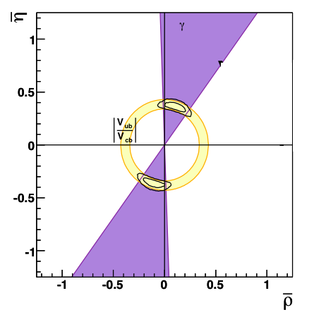
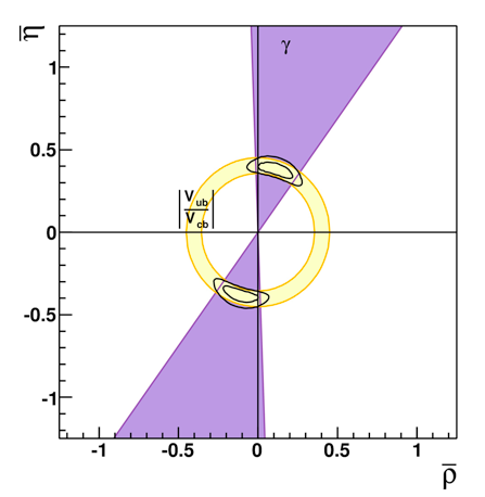
Figure 1: Result for the 2-D allowed region for the CKM parameters $\bar{\rho}$ and $\bar{\eta}$, obtained using the reference posterior for $V_{ub}$ and the LL prescription (left), or using flat priors for $\bar{\rho}$ and $\bar{\eta}$ (right).

Our second case study, which uses a simplified version of the mSUGRA model, is more complicated since Eq. 4 cannot be solved analytically in the case of a generic search for new physics. In this case, the LL domain is given by all the models predicting the same expected signal yield $s$. The expected signal yield as a function of the model parameters can be written as $s(m_{0},m_{1/2})=\epsilon(m_{0},m_{1/2})\sigma(m_{0},m_{1/2})\cal{L}$, where only the luminosity $\cal{L}$ is a constant, while both the cross section $\sigma$ and the efficiency of the applied selection $\epsilon$ depends on the features of the model (e.g. the masses of the SUSY particles), and hence on the model parameters. The function $\sigma(m_{0},m_{1/2})$ can be computed from the SUSY Lagrangian, while $\epsilon(m_{0},m_{1/2})$ has a non-trivial dependence on the models, through several effects connected to the detector response. For instance, a model with large (small) mass differences would give a large (small) value of $\epsilon$, since harder (softer) spectra for the visible particles produced in the SUSY decay chain will have larger (smaller) chance to survive the kinematic cuts. In general, the connection between the features of the model and the detector performance produces non-analytical iso-yield contours for the LL domains. This is illustrated in Fig. 2, where $\epsilon(m_{0},m_{1/2})$ and $\sigma(m_{0},m_{1/2})$ are shown in the case of a hypothetical SUSY search [9].

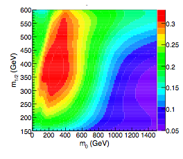
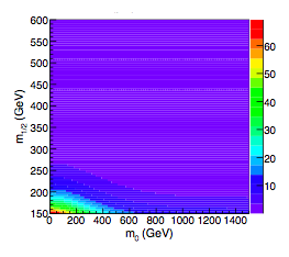
Figure 2: $\epsilon(m_{0},m_{1/2})$ and $\sigma(m_{0},m_{1/2})$ functions in the case of a hypothetical SUSY search [9].

On the other hand, all the iso-yield contours have infinite length, resulting in constant $K(m_{0},m_{1/2})$ if one considers the full domain for $m_{0}$ and $m_{1/2}$, and approximately constant if one uses a large-enough domain in practice . We can then take $K(m_{0},m_{1/2})$ as a constant and show how the method works. It has to be clearly stated that this is an approximation, and that the computation of the surface term of Eq. 4 is the main challenge in the applicability of the proposed method in its exact form (see Ref. [9] for details).

For illustration, we take the CMS low mass (LM) point [10] ($m_{0}=60$, $m_{1/2}=250)$ as the true state of nature and we simulate the case of an experiment giving a result exactly at the expectation, for low (1 pb^-1), moderate (100 pb^-1), and large (500 pb^-1) statistics. Figure 3 shows the 2-D function obtained by the LL prescription. With increasing sample size, the function shows a peak corresponding to the true value and to all its (degenerate) LL models, showing the consistency of the procedure.

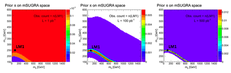
Figure 3: Result for the 2-D function mapped from the 1-D reference posterior in the case of 1 pb^-1 (left), 100 pb^-1 (center), and 500 pb^-1 (right) integrated luminosity. We assume a measurement perfectly in agreement with the expectation from the true model, corresponding to $m_{0}=60$, $m_{1/2}=250$.

4 Conclusions

We described the use of the reference prior to 1-D cases (typical of a HEP measurement) and how this can be used to define an $n$-D function of the model, induced by the 1-D reference posterior, which may then be used as a prior for further applications (e.g. to fit to model parameters). The connection between the 1-D posterior on a measurable quantity $s$ (e.g. a signal yield on top of a background $b$) and an $n$-D function of a set of interesting parameters (e.g. the parameters of a SUSY model) is established through the look-alike prescription, which defines a heuristic procedure on the basis of two minimal conditions: i) the models predicting the same expected value for the interesting variable $s$ are equi-probable and ii) the $n$-D function should map back to the 1-D reference posterior for $s$, from which we started. This requires the calculation of a surface term (see Eq. 4), which can be performed numerically [9]. While in specific cases this choice of a prior might be in conflict with a subjective assessment that could favor one region of the parameter space over another, it should be stressed that this Bayesian approach is likely to give the best frequentist performance because of the good frequentist properties of reference priors.

We provided two simplified 2-D examples to illustrate the method, for which computational complications are absent or marginal. Work is in progress to extend this procedure to more realistic cases [9].

5 Acknowledgment

The authors would like to thank J. Berger for the helpful suggestions and the interesting discussion.

References

- [1] J. Charles, A. Hocker, H. Lacker, F. R. Le Diberder, S. T’Jampens, hep-ph/0607246.
- [2] S. James Press, Subjective and objective Bayesian statistics: principles, models, and applications, John Wiley & Sons, 2003
- [3] See for instance, Berger, J. and Bernardo, J. (1992) ‘Bayesian Statistics 4’, J.M. Bernardo, et. al. (Eds.), 35-60, Oxford University Press, Oxford (and references therein).
- [4] S. Kullback, R. A. Leibler Annals of Mathematical Statistics 22, 79 (1951).
- [5] G. Sankar Datta and M. Ghosh, The Annals of Statistics, 24, 141 (1996).
- [6] L. Demortier, S. Jain, H. B. Prosper, Phys. Rev. D82 , 034002 (2010); [arXiv:1002.1111 [stat.AP]].
- [7] The CMS Collaboration, Physics Analysis Summary SUS-10-009.
- [8] M. Bona et al. [ UTfit Collaboration ], JHEP 0610 , 081 (2006); [hep-ph/0606167].
- [9] M. Pierini et al., in preparation.
- [10] The CMS Collaboration, J. Phys. G 34 (2007).