A Hilbert Scheme in Computer Vision

Abstract.

Multiview geometry is the study of two-dimensional images of three-dimensional scenes, a foundational subject in computer vision. We determine a universal Gröbner basis for the multiview ideal of $n$ generic cameras. As the cameras move, the multiview varieties vary in a family of dimension $11n-15$. This family is the distinguished component of a multigraded Hilbert scheme with a unique Borel-fixed point. We present a combinatorial study of ideals lying on that Hilbert scheme.

1. Introduction

Computer vision is based on mathematical foundations known as multiview geometry [7, 9] or epipolar geometry [11, §9]. In that subject one studies the space of pictures of three-dimensional objects seen from $n\geq 2$ cameras. Each camera is represented by a $3\times 4$-matrix $A_{i}$ of rank $3$. The matrix specifies a linear projection from ${\mathbb{P}}^{3}$ to ${\mathbb{P}}^{2}$, which is well-defined on ${\mathbb{P}}^{3}\backslash\{f_{i}\}$, where the focal point $f_{i}$ is represented by a generator of the kernel of $A_{i}$.

The space of pictures from the $n$ cameras is the image of the rational map

(1) $$\phi_{A}\,:\,\,{\mathbb{P}}^{3}\,\dashrightarrow\,({\mathbb{P}}^{2})^{n},\,\,\,\,\textbf{x}\,\mapsto\,(A_{1}\textbf{x},A_{2}\textbf{x},\ldots,A_{n}\textbf{x}).$$

The closure of this image is an algebraic variety, denoted $V_{A}$ and called the multiview variety of the given $n$-tuple of $3\times 4$-matrices $A=(A_{1},A_{2},\ldots,A_{n})$. In geometric language, the multiview variety $V_{A}$ is the blow-up of ${\mathbb{P}}^{3}$ at the cameras $f_{1},\ldots,f_{n}$, and we here study this threefold as a subvariety of $({\mathbb{P}}^{2})^{n}$.

The multiview ideal $J_{A}$ is the prime ideal of all polynomials that vanish on the multiview variety $V_{A}$. It lives in a polynomial ring $K[x,y,z]$ in $3n$ unknowns $(x_{i},y_{i},z_{i})$, $i=1,2,\ldots,n$, that serve as coordinates on $({\mathbb{P}}^{2})^{n}$. In Section 2 we give a determinantal representation of $J_{A}$ for generic $A$, and identify a universal Gröbner basis consisting of multilinear polynomials of degree $2$, $3$ and $4$. This extends previous results of Heyden and Åström [12].

The multiview ideal $J_{A}$ has a distinguished initial monomial ideal $M_{n}$ that is independent of $A$, provided the configuration $A$ is generic. Section 3 gives an explicit description of $M_{n}$ and shows that it is the unique Borel-fixed ideal with its $\mathbb{Z}^{n}$-graded Hilbert function. Following [3], we introduce the multigraded Hilbert scheme $\mathcal{H}_{n}$ which parametrizes $\mathbb{Z}^{n}$-homogeneous ideals in $K[x,y,z]$ with the same Hilbert function as $M_{n}$. We show in Section 6 that, for $n\geq 3$, $\mathcal{H}_{n}$ has a distinguished component of dimension $11n-15$ which compactifies the space of camera positions studied in computer vision. For two cameras, that space is an irreducible cubic hypersurface in $\mathcal{H}_{2}\simeq{\mathbb{P}}^{8}$.

Section 4 concerns the case when $n\leq 4$ and the focal points $f_{i}$ are among the coordinate points $(1{:}0{:}0{:}0),\ldots,(0{:}0{:}0{:}1)$. Here the multiview variety $V_{A}$ is a toric threefold, and its degenerations are parametrized by a certain toric Hilbert scheme inside $\mathcal{H}_{n}$. Each initial monomial ideal of the toric ideal $J_{A}$ corresponds to a three-dimensional mixed subdivision as seen in Figure 1. A classification of such mixed subdivisions for $n=4$ is given in Theorem 4.3.

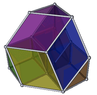
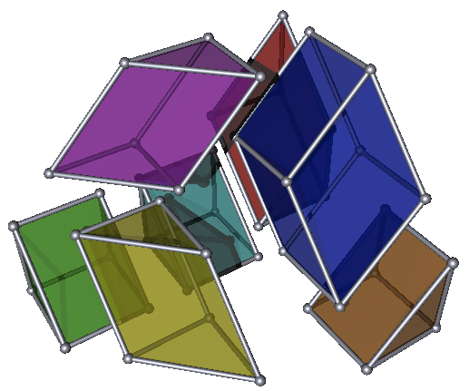
Figure 1. A multiview variety $V_{A}$ for $n=3$ cameras degenerates into six copies of ${\mathbb{P}}^{1}{\times}{\mathbb{P}}^{2}$ and one copy of ${\mathbb{P}}^{1}{\times}{\mathbb{P}}^{1}{\times}{\mathbb{P}}^{1}$.

In Section 5 we place our $n$ cameras on a line in ${\mathbb{P}}^{3}$. Moving them very close to each other on that line induces a two-step degeneration of the form

(2) $$\hbox{trinomial ideal}\ \longrightarrow\ \hbox{binomial ideal}\ \longrightarrow\ \hbox{monomial ideal}.$$

We present an in-depth combinatorial study of this curve of multiview ideals.

In Section 6 we finally define the Hilbert scheme $\mathcal{H}_{n}$, and we construct the space of camera positions as a GIT quotient of a Grassmannian. Our main result (Theorem 6.3) states that the latter is an irreducible component of $\mathcal{H}_{n}$. As a key step in the proof, the tangent space of $\mathcal{H}_{n}$ at the monomial ideal in (2) is computed and shown to have the correct dimension $11n-15$. Thus, the curve (2) consists of smooth points on the distinguished component of $\mathcal{H}_{n}$. For $n\geq 3$, our Hilbert scheme has multiple components. This is seen from our classification of monomial ideals on $\mathcal{H}_{3}$, which relates closely to [3, §5].

Acknowledgments. Aholt and Thomas thank Fredrik Kahl for hosting them at Lund in February 2011 and pointing them to the work of Heyden and Åström. They also thank Sameer Agarwal for introducing them to problems in computer vision and continuing to advise them in this field. Sturmfels thanks the Mittag-Leffler Institute, where this project started, and MATHEON Berlin for their hospitality. All three authors were partially supported by the US National Science Foundation. We are indebted to the makers of the software packages CaTS, Gfan, Macaulay2 and Sage which allowed explicit computations that were crucial in discovering our results.

2. A universal Gröbner basis

Let $K$ be any algebraically closed field, $n\geq 2$, and consider the map $\phi_{A}$ defined as in (1) by a tuple $A=(A_{1},A_{2},\ldots,A_{n})$ of $3\times 4$-matrices of rank $3$ with entries in $K$. The subvariety $V_{A}=\overline{{\rm image}(\phi_{A})}$ of $({\mathbb{P}}^{2})^{n}$ is the multiview variety, and its ideal $J_{A}\subset K[x,y,z]$ is the multiview ideal. Note that $J_{A}$ is prime because its variety $V_{A}$ is the image under $\phi_{A}$ of an irreducible variety.

We say that the camera configuration $A$ is generic if all $4\times 4$-minors of the $(4\times 3n)$-matrix $\begin{bmatrix}A_{1}^{T}\!&\!A_{2}^{T}\!&\!\cdots\!&\!A_{n}^{T}\end{bmatrix}$ are non-zero. In particular, if $A$ is generic then the focal points of the $n$ cameras are pairwise distinct in ${\mathbb{P}}^{3}$. For any subset $\sigma=\{\sigma_{1},\ldots,\sigma_{s}\}\subseteq[n]$ we consider the $3s\times(s+4)$-matrix

$$A_{\sigma}\,\,\,:=\,\,\,\begin{bmatrix}A_{\sigma_{1}}&p_{\sigma_{1}}&\mathbf{0}&\cdots&\mathbf{0}\\ A_{\sigma_{2}}&\mathbf{0}&p_{\sigma_{2}}&\ddots&\mathbf{0}\\ \vdots&\vdots&\ddots&\ddots&\vdots\\ A_{\sigma_{s}}&\mathbf{0}&\cdots&\mathbf{0}&p_{\sigma_{s}}\end{bmatrix},$$

where $p_{i}:=\begin{bmatrix}x_{i}\!&\!y_{i}\!&\!z_{i}\end{bmatrix}^{T}$ for $i\in[n]$. Assuming $s\geq 2$, each maximal minor of $A_{\sigma}$ is a homogeneous polynomial of degree $s=|\sigma|$ that is linear in $p_{i}$ for $i\in\sigma$. Thus for $s=2,3,\ldots$ these polynomials are bilinear, trilinear, etc. The matrix $A_{\sigma}$ and its maximal minors are considered frequently in multiview geometry [11, 12]. Recall that a universal Gröbner basis of an ideal is a subset that is a Gröbner basis of the ideal under all term orders. The following is the main result in this section.

Theorem 2.1.

If $A$ is generic then the maximal minors of the matrices $A_{\sigma}$ for $2\leq|\sigma|\leq 4$ form a universal Gröbner basis of the multiview ideal $J_{A}$.

The proof rests on a sequence of lemmas. Here is the most basic one.

Lemma 2.2.

The maximal minors of $A_{\sigma}$ for $|\sigma|{\geq}2$ lie in the prime ideal $J_{A}$.

Proof:   If $(p_{1},\ldots,p_{n})\in(K^{3})^{n}$ represents a point in ${\rm image}(\phi_{A})$ then there exists a non-zero vector $q\in K^{4}$ and non-zero scalars $c_{1},\ldots,c_{n}\in K$ such that $A_{i}q=c_{i}p_{i}$ for $i=1,2,\ldots,n$. This means that the columns of $A_{\sigma}$ are linearly dependent. Since $A_{\sigma}$ has at least as many rows as columns, the maximal minors of $A_{\sigma}$ must vanish at every point $p\in V_{A}$. $\square$

Later we shall see that when $A$ is generic, $J_{A}$ has only one initial monomial ideal up to symmetry. We now identify that ideal. Let $M_{n}$ denote the ideal in $K[x,y,z]$ generated by the ${n\choose 2}$ quadrics $x_{i}x_{j}$, the $3{n\choose 3}$ cubics $x_{i}y_{j}y_{k}$, and the ${n\choose 4}$ quartics $y_{i}y_{j}y_{k}y_{l}$, where $i,j,k,l$ runs over distinct indices in $[n]$.

We fix the lexicographic term order $\prec$ on $K[x,y,z]$ which is specified by $x_{1}{\succ}\cdots{\succ}x_{n}{\succ}y_{1}{\succ}\cdots{\succ}y_{n}{\succ}z_{1}{\succ}\cdots{\succ}z_{n}$. Our goal is to prove that the initial monomial ideal $\operatorname{in}_{\prec}(J_{A})$ is equal to $M_{n}$. We begin with the easier inclusion.

Lemma 2.3.

If $A$ is generic then $M_{n}\subseteq\operatorname{in}_{\prec}(J_{A})$.

Proof:   The generators of $M_{n}$ are the quadrics $x_{i}x_{j}$, the cubics $x_{i}y_{j}y_{k}$, and the quartics $y_{i}y_{j}y_{k}y_{l}$. By Lemma 2.2, it suffices to show that these are the initial monomials of maximal minors of $A_{\{ij\}}$, $A_{\{ijk\}}$ and $A_{\{ijkl\}}$ respectively.

For the quadrics this is easy. The matrix $A_{\{ij\}}$ is square and we have

(3) $${\rm det}(A_{\{ij\}})\,\,=\,\,{\rm det}\begin{bmatrix}A_{i}^{1}&\!x_{i}&\!0\\ A_{i}^{2}&\!y_{i}&\!0\\ A_{i}^{3}&\!z_{i}&\!0\\ A_{j}^{1}&\!0&\!x_{j}\\ A_{j}^{2}&\!0&\!y_{j}\\ A_{j}^{3}&\!0&\!z_{j}\end{bmatrix}\,=\,\,{\rm det}\!\begin{bmatrix}A_{i}^{2}\\ A_{i}^{3}\\ A_{j}^{2}\\ A_{j}^{3}\end{bmatrix}\!x_{i}x_{j}\,+\,\hbox{lex.~{}lower terms}.$$

where $A_{t}^{r}$ is the $r$th row of $A_{t}$. The coefficient of $x_{i}x_{j}$ is non-zero because $A$ was assumed to be generic. For the cubics, we consider the $9\times 7$-matrix

(4) $$A_{\{ijk\}}\quad=\quad\begin{bmatrix}A_{i}&p_{i}&0&0\\ A_{j}&0&p_{j}&0\\ A_{k}&0&0&p_{k}\end{bmatrix}.$$

Now, $x_{i}y_{j}y_{k}$ is the lexicographic initial monomial of the $7\times 7$-determinant formed by removing the fourth and seventh rows of $A_{\{ijk\}}$. Here we are using that, by genericity, the vectors $A_{i}^{2},A_{i}^{3},A_{j}^{3},A_{k}^{3}$ are linearly independent.

Finally, for the quartic monomial $y_{i}y_{j}y_{k}y_{l}$ we consider the $12\times 8$ matrix

(5) $$A_{\{ijkl\}}\quad=\quad\begin{bmatrix}A_{i}&p_{i}&0&0&0\\ A_{j}&0&p_{j}&0&0\\ A_{k}&0&0&p_{k}&0\\ A_{l}&0&0&0&p_{l}\end{bmatrix}.$$

Removing the first row from each of the four blocks, we obtain an $8\times 8$-matrix whose determinant has $y_{i}y_{j}y_{k}y_{l}$ as its lex. initial monomial. $\square$

The next step towards our proof of Theorem 2.1 is to express the multiview variety $V_{A}$ as a projection of a diagonal embedding of ${\mathbb{P}}^{3}$. This will put us in a position to utilize the results of Cartwright and Sturmfels in [3].

We extend each camera matrix $A_{i}$ to an invertible $4\times 4$-matrix $B_{i}=\begin{bmatrix}b_{i}\\ A_{i}\end{bmatrix}$ by adding a row $b_{i}$ at the top. Our diagonal embedding of ${\mathbb{P}}^{3}$ is the map

(6) $$\psi_{B}:{\mathbb{P}}^{3}\,\to\,({\mathbb{P}}^{3})^{n},\,\,\,\,\textbf{x}\,\mapsto\,(B_{1}\textbf{x},B_{2}\textbf{x},\ldots,B_{n}\textbf{x}).$$

Let $V^{B}:={\rm image}(\psi_{B})\subset({\mathbb{P}}^{3})^{n}$ and $J^{B}\subset K[w,x,y,z]$ its prime ideal. Here $(w_{i}:x_{i}:y_{i}:z_{i})$ are coordinates on the $i$th copy of ${\mathbb{P}}^{3}$ and $(w,x,y,z)$ are coordinates on $({\mathbb{P}}^{3})^{n}$. The ideal $J^{B}$ is generated by the $2\times 2$-minors of

(7) $$\left[B_{1}^{-1}\!\begin{bmatrix}w_{1}\\ x_{1}\\ y_{1}\\ z_{1}\end{bmatrix}\,\,B_{2}^{-1}\!\begin{bmatrix}w_{2}\\ x_{2}\\ y_{2}\\ z_{2}\end{bmatrix}\,\cdots\,\,\,B_{n}^{-1}\!\begin{bmatrix}w_{n}\\ x_{n}\\ y_{n}\\ z_{n}\end{bmatrix}\,\right].$$

This is a $4\times n$-matrix. Now consider the coordinate projection

$$\pi\,:\,({\mathbb{P}}^{3})^{n}\dashrightarrow({\mathbb{P}}^{2})^{n}\,,\,\,\,(w_{i}:x_{i}:y_{i}:z_{i})\mapsto(x_{i}:y_{i}:z_{i})\textup{ for }i=1,\ldots,n.$$

The composition $\pi\circ\psi_{B}$ is a rational map, and it coincides with $\phi_{A}$ on its domain of definition ${\mathbb{P}}^{3}\backslash\{f_{1},\ldots,f_{n}\}$. Therefore, $V_{A}=\overline{\pi(V^{B})}$ and

(8) $$J_{A}\,\,=\,\,J^{B}\cap K[x,y,z].$$

The polynomial ring $K[w,x,y,z]$ admits the natural $\mathbb{Z}^{n}$-grading $\deg(w_{i})=\deg(x_{i})=\deg(y_{i})=\deg(z_{i})=e_{i}$ where $e_{i}$ is the standard unit vector in $\mathbb{R}^{n}$. Under this grading, $K[w,x,y,z]/J^{B}$ has the multigraded Hilbert function

$$\mathbb{N}^{n}\to\mathbb{N},\,\,\,(u_{1},\ldots,u_{n})\mapsto\left(\begin{array}[]{c}u_{1}+\cdots+u_{n}+3\\ 3\end{array}\right).$$

The multigraded Hilbert scheme $H_{4,n}$ which parametrizes $\mathbb{Z}^{n}$-homogeneous ideals in $K[w,x,y,z]$ with that Hilbert function was studied in [3]. More generally, the multigraded Hilbert scheme $H_{d,n}$ represents degenerations of the diagonal ${\mathbb{P}}^{d-1}$ in $({\mathbb{P}}^{d-1})^{n}$ for any $d$ and $n$. For the general definition of multigraded Hilbert schemes see [10]. It was shown in [3] that $H_{d,n}$ has a unique Borel-fixed ideal $Z_{d,n}$. Here Borel-fixed means that $Z_{d,n}$ is stable under the action of ${\mathcal{B}}^{n}$ where ${\mathcal{B}}$ is the group of lower triangular matrices in ${\operatorname{PGL}}(d,K)$. Here is what we shall need about the monomial ideal $Z_{4,n}$.

Lemma 2.4.

(Cartwright-Sturmfels [3, §2] and Conca [4, §5])

1. The unique Borel-fixed monomial ideal $Z_{4,n}$ on $H_{4,n}$ is generated by the following monomials where $i,j,k,l$ are distinct indices in $[n]$:

   $\begin{array}[]{l}w_{i}w_{j},\,w_{i}x_{j},\,w_{i}y_{j},\,x_{i}x_{j},\,\,\,x_{i}y_{j}y_{k},\,\,y_{i}y_{j}y_{k}y_{l}.\end{array}$

2. This ideal $Z_{4,n}$ is the lexicographic initial ideal of $J^{B}$ when $B$ is sufficiently generic. The lexicographic order here is $w\succ x\succ y\succ z$ with each block ordered lexicographically in increasing order of index.

Using these results, it was deduced in [3] that all ideals on $H_{4,n}$ are radical and Cohen-Macaulay, and that $H_{4,n}$ is connected. We now use this distinguished Borel-fixed ideal $Z_{4,n}$ to prove the equality in Lemma 2.3.

Lemma 2.5.

If $A$ is generic then $M_{n}=\operatorname{in}_{\prec}(J_{A})$.

Proof:   We fix the lexicographic term order $\prec$ on $K[w,x,y,z]$ and its restriction to $K[x,y,z]$. Lemma 2.4 (1) shows that $\,M_{n}=Z_{4,n}\cap K[x,y,z]$. Lemma 2.4 (2) states that $Z_{4,n}=\operatorname{in}_{\prec}(J^{B})$ when $B$ is generic. The lexicographic order has the important property that it allows the operations of taking initial ideals and intersections to commute [5, Chapter 3]. Therefore,

$$\operatorname{in}_{\prec}(J_{A}) \,=\,\operatorname{in}_{\prec}(J^{B}\cap K[x,y,z])$$

$$\,=\,\operatorname{in}_{\prec}(J^{B})\cap K[x,y,z]$$

$$\,=\,Z_{4,n}\cap K[x,y,z]\,\,=\,\,M_{n}.$$

This identity is valid whenever the conclusion of Lemma 2.4 (2) is true. We claim that, for this to hold, the appropriate genericity notion for $B$ is that all $4\times 4$-minors of the $(4\times 4n)$-matrix $\begin{bmatrix}B_{1}^{T}\!&\!B_{2}^{T}\!&\!\cdots\!&\!B_{n}^{T}\end{bmatrix}$ are non-zero. Indeed, under this hypothesis, the maximal minors of the $4s\times(s+4)$-matrix

$$\quad B_{\sigma}\,\,\,:=\,\,\,\begin{bmatrix}B_{\sigma_{1}}&\tilde{p}_{\sigma_{1}}&\mathbf{0}&\cdots&\mathbf{0}\\ B_{\sigma_{2}}&\mathbf{0}&\tilde{p}_{\sigma_{2}}&\ddots&\mathbf{0}\\ \vdots&\vdots&\ddots&\ddots&\vdots\\ B_{\sigma_{s}}&\mathbf{0}&\cdots&\mathbf{0}&\tilde{p}_{\sigma_{s}}\end{bmatrix}\!,\,\hbox{where $\tilde{p}_{i}:=\begin{bmatrix}w_{i}\!\!&\!\!x_{i}\!\!&\!\!y_{i}\!\!&\!\!z_{i}\end{bmatrix}^{\!T}$ for $i\in[n]$,}$$

have non-vanishing leading coefficients. We see that $Z_{4,n}\subseteq\operatorname{in}_{\prec}(J^{B})$ by reasoning akin to that in the proof of Lemma 2.3. The equality $Z_{4,n}=\operatorname{in}_{\prec}(J^{B})$ is then immediate since $Z_{4,n}$ is the generic initial ideal of $J^{B}$. Hence, for any generic camera positions $A$, we can add a row to $A_{i}$ and get $B_{i}$ that are “sufficiently generic” for Lemma 2.4 (2). This completes the proof.   $\square$

Proof of Theorem 2.1: Lemma 2.5 and the proof of Lemma 2.3 show that the maximal minors of the matrices $A_{\sigma}$ for $2\leq|\sigma|\leq 4$ are a Gröbner basis of $J_{A}$ for the lexicographic term order. Each polynomial in that Gröbner basis is multilinear, thus the initial monomials remain the same for any term order satisfying $x_{i}\succ y_{i}\succ z_{i}$ for $i=1,2,\ldots,n$. So, the minors form a Gröbner basis for that term order. The set of minors is invariant under permuting $\{x_{i},y_{i},z_{i}\}$ for each $i$. Moreover, the genericity of $A$ implies that every monomial which can possibly appear in the support of a minor does so. Hence, these minors form a universal Gröbner basis of $J_{A}$. ∎

Remark 2.6.

Computer vision experts have known for a long time that multiview varieties $V_{A}$ are defined set-theoretically by the above multilinear constraints of degree at most $4$. We refer to work of Heyden and Åström [12, 13]. What is new here is that these constraints define $V_{A}$ in the strongest possible sense: they form a universal Gröbner basis for the prime ideal $J_{A}$.

The $n$ cameras are in linearly general position if no four focal points are coplanar and no three are collinear. While the number of multilinear polynomials in our lex Gröbner basis of $J_{A}$ is $\,\binom{n}{2}+3\binom{n}{3}+\binom{n}{4}$, far fewer suffice to generate the ideal $J_{A}$ when $A$ is in linearly general position.

Corollary 2.7.

If $A$ is in linearly general position then the ideal $J_{A}$ is minimally generated by $\,\binom{n}{2}$ bilinear and $\binom{n}{3}$ trilinear polynomials.

Proof:   This can be shown for $n\leq 4$ by a direct calculation. Alternatively, these small cases are covered by transforming to the toric ideals in Section 4. First map the focal points of the cameras to the torus fixed focal points of the toric case, followed by multiplying each $A_{i}$ by a suitable $g_{i}\in\operatorname{PGL}(3,K)$.

Now let $n\geq 5$. For any three cameras $i,j,k$, the maximal minors of (4) are generated by only one such maximal minor modulo the three bilinear polynomials (3). Likewise, for any four cameras $i$, $j$, $k$ and $l$, the maximal minors of (5) are generated by the trilinear and bilinear polynomials. This implies that the resulting $\binom{n}{2}+\binom{n}{3}$ polynomials generate $J_{A}$, and, by restricting to two or three cameras, we see that they minimally generate. $\square$

3. The Generic Initial Ideal

We now focus on combinatorial properties of our special monomial ideal

$$M_{n}\quad=\quad\bigl{\langle}\,x_{i}x_{j},\,x_{i}y_{j}y_{k},\,y_{i}y_{j}y_{k}y_{l}\,\,:\,\,\forall\,\,i,j,k,l\in[n]\,\,\textup{distinct}\bigr{\rangle}.$$

We refer to $M_{n}$ as the generic initial ideal in multiview geometry because it is the lex initial ideal of any multiview ideal $J_{A}$ after a generic coordinate change via the group $G^{n}$ where $G={\operatorname{PGL}}(3,K)$. Indeed, consider any rank $3$ matrices $A_{1},A_{2},\ldots,A_{n}\in K^{3\times 4}$ with pairwise distinct kernels $K\{f_{i}\}$. If $g=(g_{1},g_{2},\ldots,g_{n})$ is generic in $G^{n}$ then $g\circ A$ is generic in the sense that all $4\times 4$-minors of the matrix $\begin{bmatrix}(g_{1}A_{1})^{T}\!\!&\!\!(g_{2}A_{2})^{T}\!\!&\!\!\cdots\!\!&\!\!(g_{n}A_{n})^{T}\end{bmatrix}$ are non-zero. Thus, by the results of Section 2, $M_{n}$ is the initial ideal of $J_{g\circ A}$, or, using standard commutative algebra lingo, $M_{n}$ is the generic initial ideal of $J_{A}$.

Since $M_{n}$ is a squarefree monomial ideal, it is radical. Hence $M_{n}$ is the intersection of its minimal primes, which are generated by subsets of the variables $x_{i}$ and $y_{j}$. We begin by computing this prime decomposition.

Proposition 3.1.

The generic initial ideal $M_{n}$ is the irredundant intersection of $\binom{n}{3}+2\binom{n}{2}$ monomial primes. These are the monomial primes $P_{ijk}$ and $Q_{ij}\subseteq K[x,y,z]$ defined below for any distinct indices $i,j,k\in[n]$:

• $P_{ijk}$ is generated by $x_{1},\dots,x_{n}$ and all $y_{l}$ with $l\not\in\{i,j,k\}$,

• $Q_{ij}$ is generated by all $x_{l}$ for $l\neq i$ and $y_{l}$ for $l\not\in\{i,j\}$.

Proof:  Let $L$ denote the intersection of all $P_{ijk}$ and $Q_{ij}$. Each monomial generator of $M_{n}$ lies in $P_{ijk}$ and in $Q_{ij}$, so $M_{n}\subseteq L$. For the reverse inclusion, we will show that $V(M_{n})$ is contained in $V(L)=(\cup V(P_{ijk}))\cup(\cup V(Q_{ij}))$.

Let $(\tilde{x},\tilde{y},\tilde{z})$ be any point in the variety $V(M_{n})$. First suppose $\tilde{x}_{i}=0$ for all $i\in[n]$. Since $\tilde{y}_{i}\tilde{y}_{j}\tilde{y}_{k}\tilde{y}_{l}=0$ for distinct indices, there are at most three indices $i,j,k$ such that $\tilde{y}_{i}$, $\tilde{y}_{j}$ and $\tilde{y}_{k}$ are nonzero. Hence $(\tilde{x},\tilde{y},\tilde{z})\in V(P_{ijk})$.

Next suppose $\tilde{x}_{i}\not=0$. The index $i$ is unique because $x_{i}x_{j}\in M_{n}$ for all $j\not=i$. Since $\tilde{x}_{i}\tilde{y}_{j}\tilde{y}_{k}=0$ for all $j,k\neq i$, we have $\tilde{y}_{j}\neq 0$ for at most one index $j\neq i$. These properties imply $(\tilde{x},\tilde{y},\tilde{z})\in V(Q_{ij})$. $\square$

We regard the monomial variety $V(M_{n})$ as a threefold inside the product of projective planes $({\mathbb{P}}^{2})^{n}$. If the focal points are distinct, $V_{A}$ has a Gröbner degeneration to the reducible threefold $V(M_{n})$. The irreducible components of $V(M_{n})$ are

(9) $$V(P_{ijk})\,\simeq\,{\mathbb{P}}^{1}\times{\mathbb{P}}^{1}\times{\mathbb{P}}^{1}\quad\hbox{and}\quad V(Q_{ij})\,\simeq\,{\mathbb{P}}^{2}\times{\mathbb{P}}^{1}.$$

We find it convenient to regard $({\mathbb{P}}^{2})^{n}$ as a toric variety, so as to identify it with its polytope $(\Delta_{2})^{n}$, a direct product of triangles. The components in (9) are $3$-dimensional boundary strata of $({\mathbb{P}}^{2})^{n}$, and we identify them with faces of $(\Delta_{2})^{n}$. The corresponding $3$-dimensional polytopes are the $3$-cube and the triangular prism. The following three examples illustrate this view.

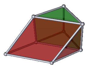
Figure 2. The variety of the generic initial ideal $M_{2}$ seen as two adjacent facets of the $4$-dimensional polytope $\Delta_{2}\times\Delta_{2}$.

Example 3.2.

[Two cameras $(n=2)$]   The variety of $\,M_{2}=\langle x_{1}\rangle\,\cap\,\langle x_{2}\rangle\,$ is a hypersurface in ${\mathbb{P}}^{2}\times{\mathbb{P}}^{2}$. The two components are triangular prisms ${\mathbb{P}}^{2}\times{\mathbb{P}}^{1}$, which are glued along a common square ${\mathbb{P}}^{1}\times{\mathbb{P}}^{1}$, as shown in Figure 2. ∎

Example 3.3.

[Three cameras $(n=3)$]   The variety of $M_{3}$ is a threefold in ${\mathbb{P}}^{2}\times{\mathbb{P}}^{2}\times{\mathbb{P}}^{2}$. Its seven components are given by the prime decomposition

$$\begin{matrix}M_{3}\quad=&\quad\langle x_{1},x_{2},y_{1}\rangle\,\cap\,\langle x_{1},x_{2},y_{2}\rangle\,\cap\,\langle x_{1},x_{3},y_{1}\rangle&\\ &\,\cap\,\,\langle x_{1},x_{3},y_{3}\rangle\,\cap\,\langle x_{2},x_{3},y_{2}\rangle\,\cap\,\langle x_{2},x_{3},y_{3}\rangle&\!\!\cap\,\,\langle x_{1},x_{2},x_{3}\rangle.\end{matrix}$$

The last component is a cube ${\mathbb{P}}^{1}\times{\mathbb{P}}^{1}\times{\mathbb{P}}^{1}$, and the other six components are triangular prisms ${\mathbb{P}}^{2}\times{\mathbb{P}}^{1}$. These are glued in pairs along three of the six faces of the cube. For instance, the two triangular prisms $V(x_{1},x_{2},y_{1})$ and $V(x_{1},x_{3},y_{1})$ intersect the cube $V(x_{1},x_{2},x_{3})$ in the common square face $V(x_{1},x_{2},x_{3},y_{1})$ $\simeq{\mathbb{P}}^{1}\times{\mathbb{P}}^{1}$. This polyhedral complex lives in the boundary of $(\Delta_{2})^{3}$, and it shown in Figure 3. Compare this picture with Figure 1. ∎

​​​​​

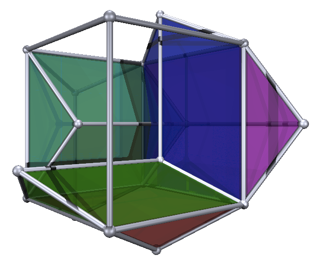
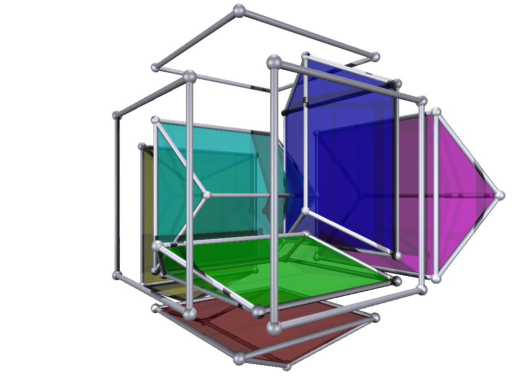
Figure 3. The monomial variety $V(M_{3})$ as a subcomplex of $(\Delta_{2})^{3}$.

Example 3.4.

[Four cameras $(n=4)$] The variety $V(M_{4})$ is a threefold in $({\mathbb{P}}^{2})^{4}$, regarded as a $3$-dimensional subcomplex in the boundary of the $8$-dimensional polytope $(\Delta_{2})^{4}$. It consists of four cubes and twelve triangular prisms. The cubes share a common vertex, any two cubes intersect in a square, and each of the six squares is adjacent to two triangular prisms. ∎

From the prime decomposition in Proposition 3.1 we can read off the multidegree [17, §8.5] of the ideal $M_{n}$. Here and in what follows, we use the natural $\mathbb{Z}^{n}$-grading on $K[x,y,z]$ given by $\deg(x_{i})=\deg(y_{i})=\deg(z_{i})=e_{i}$. Each multiview ideal $J_{A}$ is homogeneous with respect to this $\mathbb{Z}^{n}$-grading.

Corollary 3.5.

The multidegree of the generic initial ideal $M_{n}$ is equal to

(10) $$\mathcal{C}\bigl{(}K[x,y,z]/M_{n};{\bf t})\bigr{)}\,\,\,=\,\,\,t_{1}^{2}t_{2}^{2}\cdots t_{n}^{2}\cdot\left(\sum_{1\leq i<j<k\leq n}\!\frac{1}{t_{i}t_{j}t_{k}}\,+\!\sum_{1\leq i,j\leq n}\!\frac{1}{t_{i}^{2}t_{j}}\,\right)$$

A more refined analysis also yields the Hilbert function in the $\mathbb{Z}^{n}$-grading.

Theorem 3.6.

The multigraded Hilbert function of $K[x,y,z]/M_{n}$ equals

(11) $$\mathbb{N}^{n}\,\to\,\mathbb{N},\ (u_{1},\ldots,u_{n})\,\mapsto\,{u_{1}+\cdots+u_{n}+3\choose 3}-\sum_{i=1}^{n}{u_{i}+2\choose 3}.$$

Proof:  Fix $u\in\mathbb{N}^{n}$. A $K$-basis $\mathfrak{B}_{u}$ for $(K[x,y,z]/M_{n})_{u}$ is given by all monomials $x^{a}y^{b}z^{c}\not\in M_{n}$ such that $a+b+c=u$. Therefore, either (i) $a=0$ and at most three components of $b$ are non-zero; or (ii) $a\neq 0$, in which case only one $a_{i}$ can be non-zero and $b_{j}\not=0$ for at most one $j\in[n]\backslash\{i\}$.

We shall count the monomials in $\mathfrak{B}_{u}$. Monomials of type (i) look like $y^{b}z^{c}$, with at most three nonzero entries in $b$. Also, $b$ determines $c$ since $c_{i}=u_{i}-b_{i}$ for all $i\in[n]$, and so we count the number of possibilities for $y^{b}$. There are $u_{i}$ choices for $b_{i}\neq 0$, and thus $U:=u_{1}+\cdots+u_{n}$ many monomials in the set ${\mathcal{Y}}:=\{y_{i}^{b_{i}}\,:\,1\leq b_{i}\leq u_{i},\,i=1,\ldots,n\}$. The factor $y^{b}$ in $y^{b}z^{c}$ is the product of $0$, $1$, $2$ or $3$ monomials from ${\mathcal{Y}}$ with distinct subscripts.

To resolve over-counting, consider a fixed index $i$. There are ${u_{i}\choose 2}$ ways of choosing two monomials from ${\mathcal{Y}}$ with subscript $i$ and ${u_{i}\choose 3}$ ways of choosing three monomials from ${\mathcal{Y}}$ with subscript $i$. Also, there are ${u_{i}\choose 2}(U-u_{i})$ ways of choosing two monomials from ${\mathcal{Y}}$ with subscript $i$ and a third monomial with a different subscript. Hence, the number of choices for $y^{b}$ in $y^{b}z^{c}$ is

$${U\choose 0}+{U\choose 1}+\left[{U\choose 2}-\sum_{i=1}^{n}\!{u_{i}\choose 2}\right]+\left[{U\choose 3}-\sum_{i=1}^{n}\!{u_{i}\choose 3}-U\sum_{i=1}^{n}\!{u_{i}\choose 2}+\sum_{i=1}^{n}u_{i}{u_{i}\choose 2}\right]\!.$$

For case (ii) we count all monomials $x^{a}y^{b}z^{c}\in\mathfrak{B}_{u}$ with $a_{i}\neq 0$ and all other $a_{j}=0$. It suffices to count the choices for the factor $x^{a}y^{b}$. For fixed $i$, there are ${u_{i}+1\choose 2}$ monomials of the form $x_{i}^{a_{i}}y_{i}^{b_{i}}$ with $a_{i}+b_{i}\leq u_{i}$ and $a_{i}\geq 1$. Such a monomial may be multiplied with $y_{j}^{b_{j}}$ such that $j\neq i$ and $0\leq b_{j}\leq u_{j}$. This amounts to choosing zero or one monomial from ${\mathcal{Y}}\backslash\{y_{i},y_{i}^{2},\ldots,y_{i}^{u_{i}}\}$ for which there are $1+U-u_{i}$ choices. Hence, there are

$$[1+U]\sum_{i=1}^{n}{u_{i}+1\choose 2}\,-\,\sum_{i=1}^{n}u_{i}{u_{i}+1\choose 2}$$

monomials in $\mathfrak{B}_{u}$ of type (ii). Adding the two expressions, we get

$$|\mathfrak{B}_{u}| =1+U+{U\choose 2}+{U\choose 3}+(1+U)\sum_{i=1}^{n}{u_{i}\choose 1}-\sum_{i=1}^{n}u_{i}{u_{i}\choose 1}-\sum_{i=1}^{n}{u_{i}\choose 3}$$

$$=1+U+{U\choose 2}+{U\choose 3}+(1+U)U-\sum_{i=1}^{n}{u_{i}+2\choose 3}$$

$$={U+3\choose 3}-\sum_{i=1}^{n}{u_{i}+2\choose 3}.$$

$\square$

Our analysis of $M_{n}$ has the following implication for the multiview ideals $J_{A}$. Note that these are $\mathbb{Z}^{n}$-homogeneous for any camera configuration $A$.

Theorem 3.7.

For an $n$-tuple of camera matrices $A=(A_{1},\ldots,A_{n})$ with $\textup{rank}(A_{i})=3$ for each $i$, the multiview ideal $J_{A}$ has the Hilbert function (11) if and only if the focal points of the $n$ cameras are pairwise distinct.

Proof:   The if-direction follows from the argument in the first paragraph of this section. If the $n$ camera positions $f_{i}={\rm ker}(A_{i})$ are distinct in ${\mathbb{P}}^{3}$ then $M_{n}$ is the generic initial ideal of $J_{A}$, and hence both ideals have the same $\mathbb{Z}^{n}$-graded Hilbert function. For the only-if-direction we shall use:

(12) If $$Q\in\operatorname{PGL}(4,K) AQ:=(A_{1}Q,\ldots,A_{n}Q) J_{A}=J_{AQ}$$ and , then .

This holds because $Q$ defines an isomorphism on ${\mathbb{P}}^{3}$ and hence $\phi_{A}$ as in (1) has the same image in $({\mathbb{P}}^{2})^{n}$ as $\phi_{AQ}$.

Suppose first that $n=2$ and $A_{1}$ and $A_{2}$ have the same focal point and hence the same (three-dimensional) rowspace $W$. We can map $W$ to the hyperplane $\{x_{1}=0\}$ by some $Q\in\operatorname{PGL}(4,K)$, and (12) ensures that $J_{A}=J_{AQ}$. Thus we may assume that $A_{1}=\left[\begin{array}[]{ll}\bf{0}&C_{1}\end{array}\right]$ and $A_{2}=\left[\begin{array}[]{ll}\bf{0}&C_{2}\end{array}\right]$ where $C_{1}$ and $C_{2}$ are invertible matrices and $\bf{0}$ is a column of zeros. Choosing $f_{1}=f_{2}=(1,0,0,0)$ as the top row of $B_{1}$ and $B_{2}$ (as in Section 2), we have

$$B_{1}^{-1}=\left[\begin{array}[]{cc}1&\bf{0}\\ \bf{0}&C_{1}^{-1}\end{array}\right],\,\,\,B_{2}^{-1}=\left[\begin{array}[]{cc}1&\bf{0}\\ \bf{0}&C_{2}^{-1}\end{array}\right].$$

The ideal $J^{B}$ is generated by the $2\times 2$ minors of the matrix (7) which is

$$D=\left[\begin{array}[]{cc}w_{1}&w_{2}\\ p_{1}(x_{1},y_{1},z_{1})&q_{1}(x_{2},y_{2},z_{2})\\ p_{2}(x_{1},y_{1},z_{1})&q_{2}(x_{2},y_{2},z_{2})\\ p_{3}(x_{1},y_{1},z_{1})&q_{3}(x_{2},y_{2},z_{2})\end{array}\right]$$

where the $p_{i}$’s and $q_{i}$’s are linear polynomials. The ideal $I$ generated by the $2\times 2$ minors of the submatrix of $D$ obtained by deleting the top row lies on the Hilbert scheme $H_{3,2}$ from [3] and hence $K[x,y,z]/I$ has Hilbert function

$$\mathbb{N}^{2}\to\mathbb{N},\,\,\,(u_{1},u_{2})\mapsto\left(\begin{array}[]{c}u_{1}+u_{2}+2\\ 2\end{array}\right).$$

For $(u_{1},u_{2})=(1,1)$, this has value $6$. Since $I\subseteq J_{A}=J^{B}\cap K[x,y,z]$, the Hilbert function of $K[x,y,z]/J_{A}$ has value $\leq 6$, while (11) evaluates to $8$.

If $n>2$, we may assume without loss of generality that $A_{1}$ and $A_{2}$ have the same rowspace. The argument for $n=2$ shows that $J_{A}=J^{B}\cap K[x,y,z]\supseteq I$. The Hilbert function value of $K[x,y,z]/J_{A}$ in degree $e_{1}+e_{2}$ is again $8$, while the Hilbert function value of $K[x,y,z]/I$ in degree $e_{1}+e_{2}$ coincides with the value $6$ for $K[x_{1},y_{1},z_{1},x_{2},y_{2},z_{2}]/I$. So we again conclude that $K[x,y,z]/J_{A}$ does not have Hilbert function (11). $\square$

For $G=\operatorname{PGL}(3,K)$, the product $G^{n}$ acts on $K[x,y,z]$ by left-multiplication

$$(g_{1},\ldots,g_{n})\cdot\left[\begin{array}[]{c}x_{i}\\ y_{i}\\ z_{i}\end{array}\right]\,\,=\,\,\,g_{i}\left[\begin{array}[]{c}x_{i}\\ y_{i}\\ z_{i}\end{array}\right].$$

An ideal $I$ in $K[x,y,z]$ is said to be Borel-fixed if it is fixed under the induced action of ${\mathcal{B}}^{n}$ where ${\mathcal{B}}$ is the subgroup of lower triangular matrices in $G$.

Proposition 3.8.

The generic initial ideal $M_{n}$ is the unique ideal in $K[x,y,z]$ that is Borel-fixed and has the Hilbert function (11) in the $\mathbb{Z}^{n}$-grading.

Proof:  The proof is analagous to that of [3, Theorem 2.1], where $Z_{d,n}$ plays the role of $M_{n}$. The ideal $M_{n}$ is Borel-fixed because it is a generic initial ideal. The same approach as in [6, §15.9.2] can be used to prove this fact.

The multidegree of any $\mathbb{Z}^{n}$-graded ideal is determined by its Hilbert series [17, Claim 8.54]. Thus any ideal $I$ with Hilbert function (11) has multidegree (10). Let $I$ be such a Borel-fixed ideal. This is a monomial ideal.

Each maximum-dimensional associated prime $P$ of $I$ has multidegree either $t_{1}^{2}t_{2}^{2}\cdots t_{n}^{2}/(t_{i}t_{j}t_{k})$ or $t_{1}^{2}t_{2}^{2}\cdots t_{n}^{2}/(t_{i}^{2}t_{j})$, by [17, Theorem 8.53]. In the first case $P$ is generated by $2n-3$ indeterminates, one associated with each of the three cameras $i,j,k$ and two each from the other $n-3$ cameras. Borel-fixedness of $I$ tells us that the generators indexed by each camera must be the most expensive variables with respect to the order $\prec$. Hence $P=P_{ijk}$. Similarly, $P=Q_{ij}$ in the case when $P$ has multidegree $t_{1}^{2}t_{2}^{2}\cdots t_{n}^{2}/(t_{i}^{2}t_{j})$.

Every prime component of $M_{n}$ is among the minimal associated primes of $I$. This yields the containments $I\subseteq\sqrt{I}\subseteq M_{n}$. Since $I$ and $M_{n}$ have the same $\mathbb{Z}^{n}$-graded Hilbert function, the equality $I=M_{n}$ holds. $\square$

The Stanley-Reisner complex of a squarefree monomial ideal $M$ in a polynomial ring $K[t_{1},\ldots,t_{s}]$ is the simplicial complex on $\{1,\ldots,s\}$ whose facets are the sets $[s]\backslash\sigma$ where $P_{\sigma}:=\{t_{i}\,:\,i\in\sigma\}$ is a minimal prime of $M$. A shelling of a simplicial complex is an ordering $F_{1},F_{2},\ldots,F_{q}$ of its facets such that, for each $1<j\leq q$, there exists a unique minimal face of $F_{j}$ (with respect to inclusion) among the faces of $F_{j}$ that are not faces of some earlier facet $F_{i}$, $i<j$; see [18, Definition 2.1]. If the Stanley-Reisner complex of $M$ is shellable, then $K[t_{1},\ldots,t_{s}]/M$ is Cohen-Macaulay [18, Theorem 2.5].

Proposition 3.9.

The Stanley-Reisner complex of the generic initial ideal $M_{n}$ is shellable. Hence the quotient ring $K[x,y,z]/M_{n}$ is Cohen-Macaulay.

Proof:  This proof is similar to that for $Z_{d,n}$ given in [3, Corollary 2.6]. Let $\Delta_{n}$ denote the Stanley-Reisner complex of the ideal $M_{n}$. By Proposition 3.1, there are two types of minimal primes for $M_{n}$, namely $P_{ijk}$ and $Q_{ij}$, which we describe uniformly as follows. Let $P=(p_{ij})$ be the $3\times n$ matrix whose $i$th column is $[x_{i}\,\,y_{i}\,\,z_{i}]^{T}$. For $u\in\{0,1,2\}^{n}$ define $P_{u}:=\langle p_{ij}\,:\,i\leq u_{j},\,1\leq j\leq n\rangle$. Then the minimal primes $P_{ijk}$ of $M_{n}$ are precisely the primes $P_{u}$ as $u$ varies over all vectors with three coordinates equal to one and the rest equal to two, and the minimal primes $Q_{ij}$ are those $P_{u}$ where $u$ has one coordinate equal to zero, one coordinate equal to one and the rest equal to two. The facet of $\Delta_{n}$ corresponding to the minimal prime $P_{u}$ is then $F_{u}:=\{p_{ij}\,:\,u_{j}<i\leq 3,\,1\leq j\leq n\}$. We claim that the ordering of the facets $F_{u}$ induced by ordering the $u$’s lexicographically starting with $(0,1,2,2,\ldots,2)$ and ending with $(2,2,\ldots,2,1,0)$ is a shelling of $\Delta_{n}$.

Consider the face $\eta_{u}:=\{p_{ij}\,:\,j>1,i=u_{j}+1\leq 2\}$ of the facet $F_{u}$. We will prove that $\eta_{u}$ is the unique minimal one among the faces of $F_{u}$ that have not appeared in a facet $F_{u^{\prime}}$ for $u^{\prime}<u$. Suppose $G$ is a face of $F_{u}$ that does not contain $\eta_{u}$. Pick an element $p_{u_{j}+1,j}\in\eta_{u}\backslash G$. Then $j>1$, $u_{j}\leq 1$ and so if $F_{u}$ is not the first facet in the ordering, then there exists $i<j$ such that $u_{i}>0$ because $u>(0,1,2,2,\ldots,2)$ and of the form described above. Pick $i$ such that $i<j$ and $u_{i}>0$ and consider $F_{u+e_{j}-e_{i}}=F_{u}\backslash\{p_{u_{j}+1,j}\}\cup\{p_{u_{i},i}\}$. Then $u+e_{j}-e_{i}<u$ and $G$ is a face of $F_{u+e_{j}-e_{i}}$. Conversely, suppose $G$ is a face of $F_{u}$ that is also a face of $F_{u^{\prime}}$ where $u^{\prime}<u$. Since $\sum u^{\prime}_{j}=\sum u_{j}$, there exists some $j>1$ such that $u^{\prime}_{j}>u_{j}$. Therefore, $G$ does not contain $p_{u_{j}+1,j}$ which belongs to $\eta_{u}$. Therefore, $\eta_{u}$ is not contained in $G$. $\square$

4. A Toric Perspective

In this section we examine multiview ideals $J_{A}$ that are toric. For an introduction to toric ideals we refer the reader to [20]. We now assume that, for each camera $i$, each of the four torus fixed points in ${\mathbb{P}}^{3}$ either is the camera position or is mapped to a torus fixed point in ${\mathbb{P}}^{2}$. This implies $n\leq 4$. We fix $n=4$ and $f_{i}=e_{i}$ for $i=1,2,3,4$. Up to permuting and rescaling columns, our assumption implies that the configuration $A$ equals

$$\small A_{1}=\begin{bmatrix}0\!&\!1\!&\!0\!&\!0\\ 0\!&\!0\!&\!1\!&\!0\\ 0\!&\!0\!&\!0\!&\!1\end{bmatrix}\!,\,\,A_{2}=\begin{bmatrix}1\!&\!0\!&\!0\!&\!0\\ 0\!&\!0\!&\!1\!&\!0\\ 0\!&\!0\!&\!0\!&\!1\end{bmatrix}\!,\,\,A_{3}=\begin{bmatrix}1\!&\!0\!&\!0\!&\!0\\ 0\!&\!1\!&\!0\!&\!0\\ 0\!&\!0\!&\!0\!&\!1\end{bmatrix}\!,\,\,A_{4}=\begin{bmatrix}1\!&\!0\!&\!0\!&\!0\\ 0\!&\!1\!&\!0\!&\!0\\ 0\!&\!0\!&\!1\!&\!0\end{bmatrix}\!.$$

For this camera configuration, the multiview ideal $J_{A}$ is indeed a toric ideal:

Proposition 4.1.

The ideal $J_{A}$ is obtained by eliminating the diagonal unknowns $w_{1}$, $w_{2}$, $w_{3}$ and $w_{4}$ from the ideal of $2\times 2$-minors of the $4\times 4$-matrix

(13) $$\begin{pmatrix}w_{1}&x_{2}&x_{3}&x_{4}\\ x_{1}&w_{2}&y_{3}&y_{4}\\ y_{1}&y_{2}&w_{3}&z_{4}\\ z_{1}&z_{2}&z_{3}&w_{4}\end{pmatrix}.$$

This toric ideal is minimally generated by six quadrics and four cubics:

$$\!\begin{matrix}J_{A}\,=\,\langle y_{1}y_{4}{-}x_{1}z_{4},y_{3}x_{4}{-}x_{3}y_{4},y_{2}x_{4}{-}x_{2}z_{4},z_{1}y_{3}{-}x_{1}z_{3},z_{2}x_{3}{-}x_{2}z_{3},z_{1}y_{2}{-}y_{1}z_{2},\\ \qquad\quad y_{2}z_{3}y_{4}-z_{2}y_{3}z_{4},\,y_{1}z_{3}x_{4}-z_{1}x_{3}z_{4},\,x_{1}z_{2}x_{4}-z_{1}x_{2}y_{4},\,x_{1}y_{2}x_{3}-y_{1}x_{2}y_{3}\rangle\end{matrix}$$

Proof:   We extend $A_{i}$ to a $4\times 4$-matrix $B_{i}$ as in Section 2 by adding the row $b_{i}=e_{i}^{T}$. The $B_{i}$’s are then all permutation matrices, and the matrix in (7) equals the matrix in (13). The ideal $J^{B}$ is generated by the $2\times 2$ minors of that matrix of unknowns. The multiview ideal is $J_{A}=J^{B}\cap K[x,y,z]$. We find the listed binomial generators by performing the elimination with a computer algebra package such as Macaulay2. Toric ideals are precisely those prime ideals generated by binomials and hence $J_{A}$ is a toric ideal. $\square$

Remark 4.2.

The normalized coordinate system in multiview geometry proposed by Heyden and Åström [12] is different from ours and does not lead to toric varieties. Indeed, if one uses the camera matrices in [12, §2.3], then $J_{A}$ is also generated by six quadrics and four cubics, but seven of the ten generators are not binomials. One of the cubic generators has six terms. ∎

In commutative algebra, it is customary to represent toric ideals by integer matrices. Given $\mathcal{A}\in\mathbb{N}^{p\times q}$ with columns $a_{1},\ldots,a_{q}$, the toric ideal of $\mathcal{A}$ is

$$I_{\mathcal{A}}\,\,:=\,\,\langle t^{u}-t^{v}\,:\,\mathcal{A}u\,\,=\,\,\mathcal{A}v,\,u,v\in\mathbb{N}^{q}\rangle\,\,\subset\,\,K[t]\,:=\,K[t_{1},\ldots,t_{q}],$$

where $t^{u}$ represents the monomial $t_{1}^{u_{1}}t_{2}^{u_{2}}\cdots t_{q}^{u_{q}}$. If $\mathcal{A^{\prime}}$ is the submatrix of $\mathcal{A}$ obtained by deleting the columns indexed by $j_{1},\ldots,j_{s}$ for some $s<q$, then the toric ideal $I_{\mathcal{A^{\prime}}}$ equals the elimination ideal $I_{\mathcal{A}}\cap K[t_{j}\,:\,j\not\in\{j_{1},\ldots,j_{s}\}]$; see [20, Prop. 4.13 (a)]. The integer matrix $\mathcal{A}$ for our toric multiview ideal $J_{A}$ in Proposition 4.1 is the following Cayley matrix of format $8\times 12$:

$$\mathcal{A}\,\,\,=\,\,\,\begin{bmatrix}A_{1}^{T}&A_{2}^{T}&A_{3}^{T}&A_{4}^{T}\\ {\bf 1}&{\bf 0}&{\bf 0}&{\bf 0}\\ {\bf 0}&{\bf 1}&{\bf 0}&{\bf 0}\\ {\bf 0}&{\bf 0}&{\bf 1}&{\bf 0}\\ {\bf 0}&{\bf 0}&{\bf 0}&{\bf 1}\end{bmatrix}$$

where ${\bf 1}=[1\,1\,1]$ and ${\bf 0}=[0\,0\,0]$. This matrix $\mathcal{A}$ is obtained from the following $8\times 16$ matrix by deleting columns $1,6,11$ and $16$:

(14) $$\begin{bmatrix}I_{4}&I_{4}&I_{4}&I_{4}\\ {\bf 1}&{\bf 0}&{\bf 0}&{\bf 0}\\ {\bf 0}&{\bf 1}&{\bf 0}&{\bf 0}\\ {\bf 0}&{\bf 0}&{\bf 1}&{\bf 0}\\ {\bf 0}&{\bf 0}&{\bf 0}&{\bf 1}\end{bmatrix}$$

The vectors ${\bf 1}$ and ${\bf 0}$ now have length four, $I_{4}$ is the $4\times 4$ identity matrix and we assume that the columns of (14) are indexed by

$$w_{1},x_{1},y_{1},z_{1},x_{2},w_{2},y_{2},z_{2},x_{3},y_{3},w_{3},z_{3},x_{4},y_{4},z_{4},w_{4}.$$

The matrix (14) represents the direct product of two tetrahedra, and its toric ideal is known (by [20, Prop. 5.4]) to be generated by the $2\times 2$ minors of (13). Its elimination ideal in the ring $K[x,y,z]$ is $I_{\mathcal{A}}$, and hence $J_{A}=I_{\mathcal{A}}$.

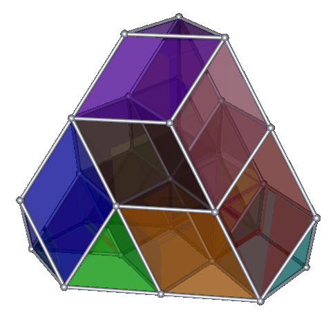
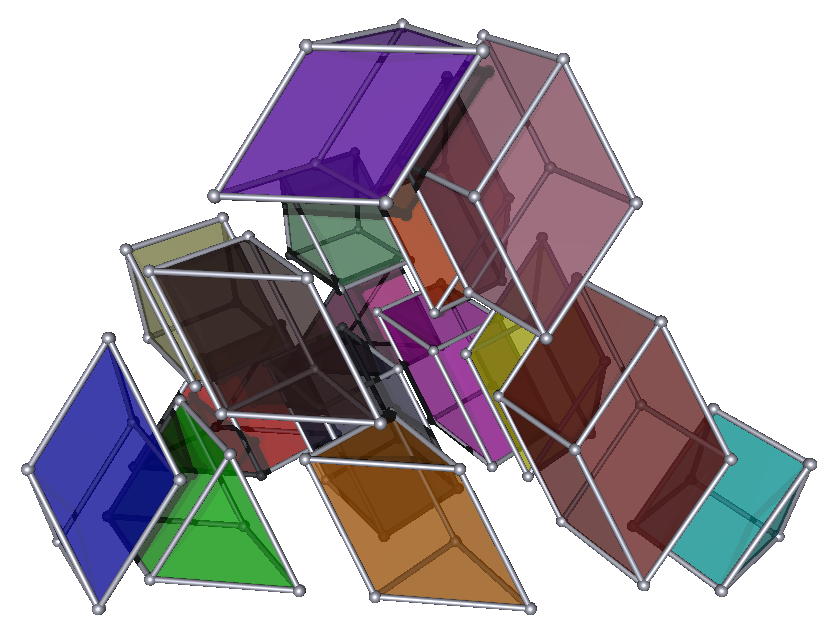
Figure 4. Initial monomial ideals of the toric multiview variety correspond to mixed subdivisions of the truncated tetrahedron $P$. These have $4$ cubes and $12$ triangular prisms.

The matrix $\mathcal{A}$ has rank $7$ and its columns determine a $6$-dimensional polytope ${\rm conv}(\mathcal{A})$ with $12$ vertices. The normalized volume of ${\rm conv}(\mathcal{A})$ equals $16$, and this is the degree of the $6$-dimensional projective toric variety in ${\mathbb{P}}^{11}$ defined by $J_{A}$. In our context, we don’t care for the $6$-dimensional variety in ${\mathbb{P}}^{11}$ but we are interested in the threefold in ${\mathbb{P}}^{2}{\times}{\mathbb{P}}^{2}{\times}{\mathbb{P}}^{2}{\times}{\mathbb{P}}^{2}$ cut out by $J_{A}$. To study this combinatorially, we apply the Cayley trick. This means we replace the $6$-dimensional polytope ${\rm conv}(\mathcal{A})$ by the $3$-dimensional polytope

$$P\,\,=\,\,{\rm conv}(A_{1}^{T})+{\rm conv}(A_{2}^{T})+{\rm conv}(A_{3}^{T})+{\rm conv}(A_{4}^{T}).$$

This is the Minkowski sum of the four triangles that form the facets of the standard tetrahedron. Equivalently, $P$ is the scaled tetrahedron $4\Delta_{3}$ with its vertices sliced off. Triangulations of $\mathcal{A}$ correspond to mixed subdivisions of $P$. Each $6$-simplex in $\mathcal{A}$ becomes a cube or a triangular prism in $P$. Each mixed subdivision has four cubes ${\mathbb{P}}^{1}\times{\mathbb{P}}^{1}\times{\mathbb{P}}^{1}$ and twelve triangular prisms ${\mathbb{P}}^{2}\times{\mathbb{P}}^{1}$. Such a mixed subdivision of $P$ is shown in Figure 4. Note the similarities and differences relative to the complex $V(M_{4})$ in Example 3.4.

We worked out a complete classification of all mixed subdivisions of $P$:

Theorem 4.3.

The truncated tetrahedron $P$ has $1068$ mixed subdivisions, one for each triangulation of the Cayley polytope ${\rm conv}(\mathcal{A})$. Precisely $1002$ of the $1068$ triangulations are regular. The regular triangulations form $48$ symmetry classes, and the non-regular triangulations form $7$ symmetry classes.

We offer a brief discussion of this result and how it was obtained. Using the software Gfan [15], we found that $I_{\mathcal{A}}$ has 1002 distinct monomial initial ideals. These ideals fall into 48 symmetry classes under the natural action of $(S_{3})^{4}\rtimes S_{4}$ on $K[x,y,z]$ where the $i$-th copy of $S_{3}$ permutes the variables $x_{i},y_{i},z_{i}$, and $S_{4}$ permutes the labels of the cameras. The matrix $\mathcal{A}$ being unimodular, each initial ideal of $I_{\mathcal{A}}$ is squarefree and each triangulation of $\mathcal{A}$ is unimodular. To calculate all non-regular triangulations, we used the bijection between triangulations and $\mathcal{A}$-graded monomial ideals in [20, Lemma 10.14]. Namely, we ran a second computation using the software package CaTS [14] that lists all $\mathcal{A}$-graded monomials ideals, and we found their number to be $1068$, and hence $\mathcal{A}$ has 66 non-regular triangulations.

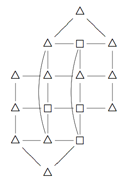
Figure 5. The dual graph of the mixed subdivision given by $Y_{1}$.

The $48$ distinct initial monomial ideals of the toric multiview ideal $J_{A}$ can be distinguished by various invariants. First, their numbers of generators range from $12$ to $15$. There is precisely one initial ideal with $12$ generators:

$$Y_{1}\,\,\,=\,\,\, \langle\,y_{1}z_{2},z_{1}y_{3},x_{1}z_{4},z_{2}x_{3},y_{2}x_{4},x_{3}y_{4},$$

$$\,\,\,\,x_{1}y_{2}x_{3},z_{1}y_{2}x_{3},x_{1}z_{2}x_{4},z_{1}x_{3}z_{4},z_{2}y_{3}x_{4},z_{2}y_{3}z_{4}\,\rangle.$$

At the other extreme, there are two classes of initial ideals with $15$ generators. These are the only classes having quartic generators, as all ideals with $\leq 14$ generators require only quadrics and cubics. A representative is

$$Y_{2}\,\,\,=\,\,\, \langle\,z_{1}y_{2},x_{1}z_{3},x_{1}z_{4},x_{2}z_{3},y_{2}x_{4},y_{3}x_{4},\,y_{1}z_{2}x_{3}y_{4},$$

$$\,\,\,\,x_{1}y_{2}x_{3},x_{1}z_{2}x_{3},x_{1}z_{2}x_{4},x_{4}z_{2}y_{1},y_{1}z_{3}x_{4},y_{1}z_{3}y_{4},y_{2}x_{3}y_{4},y_{2}z_{3}y_{4}\,\rangle.$$

All non-regular $\mathcal{A}$-graded monomial ideal have $14$ generators. One of them is

$$Y_{3}\,\,\,=\,\,\, \langle\,z_{1}y_{2},z_{1}y_{3},x_{1}z_{4},x_{2}z_{3},x_{2}z_{4},y_{3}x_{4},\,x_{1}y_{2}z_{3},y_{1}x_{2}y_{3},$$

$$\,\,\,\,x_{1}y_{2}x_{4},x_{1}z_{2}x_{4},x_{1}z_{3}x_{4},y_{1}z_{3}x_{4},y_{2}z_{3}x_{4},y_{2}z_{3}y_{4}\,\rangle.$$

A more refined combinatorial invariant of the $55$ types is the dual graph of the mixed subdivision of $P$. The $16$ vertices of this graph are labeled with squares and triangles to denote cubes and triangular prisms respectively, and edges represent common facets. The graph for $Y_{1}$ is shown in Figure 5.

For complete information on the classification in Theorem 4.3 see the website  www.math.washington.edu/$\sim$aholtc/HilbertScheme.

That website also contains the same information for the toric multiview variey in the easier case of $n=3$ cameras. Taking $A_{1},A_{2}$ and $A_{3}$ as camera matrices, the corresponding Cayley matrix has format $7\times 9$ and rank $6$:

$$\mathcal{A}\,\,\,=\,\,\,\begin{bmatrix}A_{1}^{T}&A_{2}^{T}&A_{3}^{T}\\ {\bf 1}&{\bf 0}&{\bf 0}\\ {\bf 0}&{\bf 1}&{\bf 0}\\ {\bf 0}&{\bf 0}&{\bf 1}\end{bmatrix}\,\,\,=\,\,\,\begin{bmatrix}\,0&0&0&1&0&0&1&0&0\,\\ \,1&0&0&0&0&0&0&1&0\,\\ \,0&1&0&0&1&0&0&0&0\,\\ \,0&0&1&0&0&1&0&0&1\,\\ \,1&1&1&0&0&0&0&0&0\,\\ \,0&0&0&1&1&1&0&0&0\,\\ \,0&0&0&0&0&0&1&1&1\,\end{bmatrix}$$

This is the transpose of the matrix $A_{\{123\}}$ in (4) when evaluated at $x_{1}=y_{1}=\cdots=z_{3}=1$. The corresponding $6$-dimensional Cayley polytope ${\rm conv}(\mathcal{A})$ has $9$ vertices and normalized volume $7$, and the toric multiview ideal equals

(15) $$J_{A}\,\,=\,\,\langle z_{1}y_{3}-x_{1}z_{3},z_{2}x_{3}-x_{2}z_{3},z_{1}y_{2}-y_{1}z_{2},x_{1}y_{2}x_{3}-y_{1}x_{2}y_{3}\rangle.$$

We note that the quadrics cut out $V_{A}$ plus an extra component ${\mathbb{P}}^{1}\times{\mathbb{P}}^{1}\times{\mathbb{P}}^{1}$:

(16) $$\langle z_{1}y_{3}-x_{1}z_{3},z_{2}x_{3}-x_{2}z_{3},z_{1}y_{2}-y_{1}z_{2}\rangle\,\,=\,\,J_{A}\cap\langle z_{1},z_{2},z_{3}\rangle$$

This equation is precisely [12, Theorem 5.6] but written in toric coordinates.

The toric ideal $J_{A}$ has precisely $20$ initial monomial ideals, in three symmetry classes, one for each mixed subdivision of the $3$-dimensional polytope

$$P\,\,=\,\,{\rm conv}(A_{1}^{T})+{\rm conv}(A_{2}^{T})+{\rm conv}(A_{3}^{T}).$$

Thus $P$ is the Minkowski sum of three of the four triangular facets of the regular tetrahedron. Each mixed subdivision of $P$ uses one cube ${\mathbb{P}}^{1}\times{\mathbb{P}}^{1}\times{\mathbb{P}}^{1}$ and six triangular prisms ${\mathbb{P}}^{2}\times{\mathbb{P}}^{1}$. A picture of one of them is seen in Figure 1.

Remark 4.4.

Our toric study in this section is universal in the sense that every multiview variety $V_{A}$ for $n\leq 4$ cameras in linearly general position in ${\mathbb{P}}^{3}$ is isomorphic to the toric multiview variety under a change of coordinates in $({\mathbb{P}}^{2})^{n}$. This fact can be proved using the coordinate systems for the Grassmannian ${\rm Gr}(4,3n)$ furnished by the construction in [21, §4]. Here is how it works for $n=4$. The coordinate change via ${\operatorname{PGL}}(3,K)^{4}$ gives

(17) $$\,\,\begin{bmatrix}A_{1}^{T}\!&\!A_{2}^{T}\!&\!A_{3}^{T}\!&\!A_{4}^{T}\end{bmatrix}\,\,=\,\,\left[\,\begin{matrix}0&0&0\\ *&*&*\\ *&*&*\\ *&*&*\\ \end{matrix}\quad\,\,\begin{matrix}*&*&*\\ 0&0&0\\ *&*&*\\ *&*&*\\ \end{matrix}\quad\,\,\begin{matrix}*&*&*\\ *&*&*\\ 0&0&0\\ *&*&*\\ \end{matrix}\quad\,\,\begin{matrix}*&*&*\\ *&*&*\\ *&*&*\\ 0&0&0\\ \end{matrix}\,\right]\!,$$

where the $3\times 3$-matrices indicated by the stars in the four blocks are invertible. Now, the $4\times 12$-matrix (17) gives a support set $\Sigma$ that satisfies the conditions in [21, Proposition 3.1]. The corresponding Zariski open set $\mathcal{U}_{\Sigma}$ of the Grassmannian ${\rm Gr}(4,12)$ is non-empty. In fact, by [21, Remark 4.9(a)], the set $\mathcal{U}_{\Sigma}$ represents configurations whose cameras $f_{1},f_{2},f_{3},f_{4}$ are not coplanar. Now, Theorem 4.6 in [21] completes our proof because (the universal Gröbner basis of) the ideal $J_{A}$ depends only on the point in $\mathcal{U}_{\Sigma}\subset{\rm Gr}(4,12)$ represented by (17) and not on the specific camera matrices $A_{1},\ldots,A_{4}$. ∎

5. Degeneration of Collinear Cameras

In this section we consider a family of collinear camera positions. The degeneration of the associated multiview variety will play a key role in proving our main results in Section 6, but they may be of independent interest. Collinear cameras have been studied in computer vision, for example in [11].

Let $\varepsilon$ be a parameter and fix the configuration $A(\varepsilon):=(A_{1},\ldots,A_{n})$ where

$$A_{i}\,:=\ \left[\begin{array}[]{cccc}1&1&0&0\\ 1&0&1&0\\ \varepsilon^{n-i}&0&0&1\end{array}\right]$$

The focal point of camera $i$ is $f_{i}=(-1:1:1:\varepsilon^{n-i})$ and hence the $n$ cameras given by $A(\varepsilon)$ are collinear in ${\mathbb{P}}^{3}$. Note that these camera matrices stand in sharp contrast to those for which $A$ is generic which was the focus of Sections 2 and 3. They also differ from the toric situation in Section 4.

We consider the multiview ideal $J_{A(\varepsilon)}$ in the polynomial ring $K(\varepsilon)[x,y,z]$, where $K(\varepsilon)$ is the field of rational functions in $\varepsilon$ with coefficients in $K$. Then $J_{A(\varepsilon)}$ has the Hilbert function (11), by Theorem 3.7. Let $\mathcal{G}_{n}$ be the set of polynomials in $K(\varepsilon)[x,y,z]$ consisting of the ${n\choose 2}$ quadratic polynomials

(18) $$x_{i}y_{j}-x_{j}y_{i}\qquad\hbox{for}\,\,\,\,1\leq i<j\leq n$$

and the $3{n\choose 3}$ cubic polynomials below for all choices of $1\leq i<j<k\leq n$:

(19) $$\begin{array}[]{c}(\varepsilon^{n-k}-\varepsilon^{n-i})x_{i}z_{j}x_{k}+(\varepsilon^{n-j}-\varepsilon^{n-k})z_{i}x_{j}x_{k}+(\varepsilon^{n-i}-\varepsilon^{n-j})x_{i}x_{j}z_{k}\\ (\varepsilon^{n-k}-\varepsilon^{n-i})y_{i}z_{j}y_{k}+(\varepsilon^{n-j}-\varepsilon^{n-k})z_{i}y_{j}y_{k}+(\varepsilon^{n-i}-\varepsilon^{n-j})y_{i}y_{j}z_{k}\\ (\varepsilon^{n-k}-\varepsilon^{n-i})y_{i}z_{j}x_{k}+(\varepsilon^{n-j}-\varepsilon^{n-k})z_{i}y_{j}x_{k}+(\varepsilon^{n-i}-\varepsilon^{n-j})y_{i}x_{j}z_{k}\end{array}$$

Let $L_{n}$ be the ideal generated by (18) and the following binomials from the first two terms in (19):

$$L_{n}\,:=\,\bigl{\langle}x_{i}y_{j}-x_{j}y_{i}\,:\,1{\leq}i{<}j{\leq}n\bigr{\rangle}+\left\langle\begin{array}[]{c}\!x_{i}z_{j}x_{k}-z_{i}x_{j}x_{k},\\ \!y_{i}z_{j}y_{k}-z_{i}y_{j}y_{k},\\ \!y_{i}z_{j}x_{k}-z_{i}y_{j}x_{k}\end{array}:\,1{\leq}i{<}j{<}k{\leq}n\right\rangle\!.$$

Let $N_{n}$ be the ideal generated by the leading monomials in (18) and (19):

$$N_{n}\,\,:=\,\,\bigl{\langle}x_{i}y_{j}\,:\,1{\leq}i{<}j{\leq}n\bigr{\rangle}\,+\,\bigl{\langle}x_{i}z_{j}x_{k},\,y_{i}z_{j}y_{k},\,y_{i}z_{j}x_{k}\,:\,1{\leq}i{<}j{<}k{\leq}n\bigr{\rangle}.$$

The main result in this section is the following construction of a two-step flat degeneration $J_{A(\varepsilon)}\rightarrow L_{n}\rightarrow N_{n}$. This gives an explicit realization of (2). We note that $V_{A(\varepsilon)}$ can be seen as a variant of the Mustafin varieties in [2].

Theorem 5.1.

The three ideals $J_{A(\varepsilon)}$, $L_{n}$ and $N_{n}$ satisfy the following:

1. The multiview ideal $J_{A(\varepsilon)}$ is generated by the set $\,\mathcal{G}_{n}$.

2. The binomial ideal $L_{n}$ equals the special fiber of $J_{A(\varepsilon)}$ for $\varepsilon=0$.

3. The monomial ideal $N_{n}$ is the initial ideal of $L_{n}$, in the Gröbner basis sense, with respect to the lexicographic term order with $x\succ y\succ z$.

The rest of this section is devoted to explaining and proving these results. Let us begin by showing that $\mathcal{G}_{n}$ is a subset of $J_{A(\varepsilon)}$. The determinant of

$$A(\varepsilon)_{\{ij\}}\,\,=\,\,\left[\begin{array}[]{ccc}A_{i}&p_{i}&\bf{0}\\ A_{j}&\bf{0}&p_{j}\end{array}\right]$$

equals $(\varepsilon^{n-j}-\varepsilon^{n-i})(x_{i}y_{j}-x_{j}y_{i})$. Hence $J_{A(\varepsilon)}$ contains (18), by the argument in Lemma 2.2. Similarly, for any $1{\leq}i{<}j{<}k{\leq}n$, consider the $9\times 7$ matrix

$$A(n)_{\{ijk\}}\,\,=\,\,\left[\begin{array}[]{ccccccc}1&1&0&0&x_{i}&0&0\\ 1&0&1&0&y_{i}&0&0\\ \varepsilon^{n-i}&0&0&1&z_{i}&0&0\\ 1&1&0&0&0&x_{j}&0\\ 1&0&1&0&0&y_{j}&0\\ \varepsilon^{n-j}&0&0&1&0&z_{j}&0\\ 1&1&0&0&0&0&x_{k}\\ 1&0&1&0&0&0&y_{k}\\ \varepsilon^{n-k}&0&0&1&0&0&z_{k}\end{array}\right].$$

The three cubics (19), in this order and up to sign, are the determinants of the $7\times 7$ submatrices of $A(\varepsilon)_{\{ijk\}}$ obtained by deleting the rows corresponding to $y_{j}$ and $y_{k}$, the rows corresponding to $x_{j}$ and $x_{k}$, and the rows corresponding to $x_{i}$ and $y_{k}$ respectively. We conclude that $\mathcal{G}_{n}$ lies in $J_{A(\varepsilon)}$.

We next discuss part (b) of Theorem 5.1. Every rational function $c(\varepsilon)\in K(\varepsilon)$ has a unique expansion as a Laurent series $c_{1}\varepsilon^{a_{1}}+c_{2}\varepsilon^{a_{2}}+\cdots$ where $c_{i}\in K$ and $a_{1}<a_{2}<\cdots$ are integers. The function ${\rm val}:K(\varepsilon)\rightarrow\mathbb{Z}$ given by $c(\varepsilon)\mapsto a_{1}$ is then a valuation on $K(\varepsilon)$, and $K[\![\varepsilon]\!]=\{c\in K(\varepsilon)\,:\,{\rm val}(c)\geq 0\}$ is its valuation ring. The unique maximal ideal in $K[\![\varepsilon]\!]$ is $m=\langle c\in K(\varepsilon)\,:\,{\rm val}(c)>0\rangle$. The residue field $K[\![\varepsilon]\!]/m$ is isomorphic to $K$, so there is a natural map $K[\![\varepsilon]\!]\rightarrow K$ that represents the evaluation at $\varepsilon=0$. The special fiber of an ideal $I\subset K(\varepsilon)[x,y,z]$ is the image of $I\cap K[\![\varepsilon]\!][x,y,z]$ under the induced map $K[\![\varepsilon]\!][[x,y,z]\rightarrow K[x,y,z]$. The special fiber is denoted ${\rm in}(I)$. It can be computed from $I$ by a variant of Gröbner bases (cf. [16, §2.4]).

What we are claiming in Theorem 5.1 (b) is the following identify

$${\rm in}(J_{A(\varepsilon)})\,\,=\,\,L_{n}\qquad{\rm in}\,\,K[x,y,z].$$

It is easy to see that the left hand side contains the right hand side: indeed, by multiplying the trinomials in (19) by $\varepsilon^{k-n}$ and then evaluating at $\varepsilon=0$, we obtain the binomial cubics among the generators of $L_{n}$.

Finally, what is claimed in Theorem 5.1 (c) is the following identity

$${\rm in}_{\prec}(L_{n})\,\,=\,\,N_{n}\qquad{\rm in}\,\,K[x,y,z].$$

Here, ${\rm in}_{\prec}(L_{n})$ is the lexicographic initial ideal of $L_{n}$, in the usual Gröbner basis sense. Again, the left hand side contains the right hand side because the initial monomials of the binomial generators of $L_{n}$ generate $N_{n}$.

Note that $N_{n}$ is distinct from the generic initial ideal $M_{n}$. Even though $M_{n}$ played a prominent role in Sections 2 and 3, the ideal $N_{n}$ will be more useful in Section 6. The reason is that $M_{n}$ is the most singular point on the Hilbert scheme $\mathcal{H}_{n}$ while, as we shall see, $N_{n}$ is a smooth point on $\mathcal{H}_{n}$.

In summary, what we have shown thus far is the following inclusion:

(20) $$N_{n}\,\,\subseteq\,\,{\rm in}_{\prec}\bigl{(}{\rm in}(J_{A(\varepsilon)})\bigr{)}$$

We seek to show that equality holds. Our proof rests on the following lemma.

Lemma 5.2.

The monomial ideal $N_{n}$ has the $\mathbb{Z}^{n}$-graded Hilbert function (11).

Proof:   Let $u=(u_{1},\ldots,u_{n})\in\mathbb{N}^{n}$, and let $\mathfrak{B}_{u}$ be the set of all monomials of multidegree $u$ in $K[x,y,z]$ which are not in $N_{n}$. We need to show that

$$|\mathfrak{B}_{u}|\,=\,{u_{1}+\cdots+u_{n}+3\choose 3}-\sum_{i=1}^{n}{u_{i}+2\choose 3}.$$

It can be seen from the generators of $N_{n}$ that the monomials in $\mathfrak{B}_{u}$ are of the form $z^{a}y^{b}x^{c}z^{d}$ for $a,b,c,d\in\mathbb{N}^{n}$ such that $u=a+b+c+d$ and

$$a =(a_{1},\ldots,a_{i},0,\ldots,0)$$

$$b =(0,\ldots,0,b_{i},\ldots,b_{j},0,\ldots,0)$$

$$c =(0,\ldots,0,c_{j},\ldots,c_{k},0,\ldots,0)$$

$$d =(0,\ldots,0,d_{k},\ldots,d_{n})$$

for some triple $i,j,k$ with $1\leq i\leq j\leq k\leq n$.

We count the monomials in $\mathfrak{B}_{u}$ using a combinatorial “stars and bars” argument. Each monomial can be formed in the following way. Suppose there are $u_{1}+\cdots+u_{n}+3$ blank spaces laid left to right. Fill exactly three spaces with bars. This leaves $u_{1}+\cdots+u_{n}$ open blanks to fill in, which is the total degree of a monomial in $\mathfrak{B}_{u}$. The three bars separate the blanks into four compartments, some possibly empty. From these compartments we greedily form $a$, $b$, $c$, and $d$ to make $z^{a}y^{b}x^{c}z^{d}$ as described below.

In what follows, $\star$ is used as a placeholder symbol. Fill the first $u_{1}$ blanks with the symbol $\star_{1}$, the next $u_{2}$ blanks with $\star_{2}$, and continue to fill up until the last $u_{n}$ blanks are filled with $\star_{n}$. Now we pass once more through these symbols and replace each $\star_{i}$ with either $x_{i}$, $y_{i}$, or $z_{i}$ such that all variables in the first compartment are $z$’s, those in the second are $y$’s, then $x$’s and in the fourth compartment $z$’s. Removing the bars gives $z^{a}y^{b}x^{c}z^{d}$ in $\mathfrak{B}_{u}$.

There are $\displaystyle{u_{1}+\cdots+u_{n}+3\choose 3}$ ways of choosing the three bars. The monomials in $\mathfrak{B}_{u}$ are overcounted only when $i=j=k$ if $z_{i}$ appears in both the first and fourth compartments. Indeed, in such cases if we require $a_{i}=0$, the monomial is uniquely represented, so we are overcounting by the $\displaystyle{u_{i}+2\choose 3}$ choices when $a_{i}\neq 0$. $\square$

We are now prepared to derive the main result of this section.

Proof of Theorem 5.1: Lemma 5.2 and Theorem 3.7 tell us that $N_{n}$ and $J_{A(\varepsilon)}$ have the same $\mathbb{Z}^{n}$-graded Hilbert function (11). We also know from [16, §2.4] that $\operatorname{in}(J_{A(\varepsilon)})$ has the same Hilbert function, just as passing to an initial monomial ideal for a term order preserves Hilbert function. Hence the equality $N_{n}\,\,\subseteq\,\,{\rm in}_{\prec}\bigl{(}{\rm in}(J_{A(\varepsilon)})\bigr{)}$ holds in (20). This proves parts (b) and (c). We have shown that $\mathcal{G}_{n}$ is a Gröbner basis for the homogeneous ideal $J_{A(\varepsilon)}$ in the valuative sense of [16, §2.4]. This implies that $\mathcal{G}_{n}$ generates $J_{A(\varepsilon)}$. ∎

Remark 5.3.

The polyhedral subcomplexes of $(\Delta_{2})^{n}$ defined by the binomial ideal $L_{n}$ and the monomial ideal $N_{n}$ are combinatorially interesting. For instance, $L_{n}$ has prime decomposition $I_{3}\cap I_{4}\cap\cdots\cap I_{n}\cap I_{n+1}$, where

$$I_{t}\,\, :=\,\langle\,x_{i},y_{i}:\,i=t,t+1,\ldots,n\,\rangle\ +$$

$$\ \ \ \ \ \langle\,x_{i}y_{j}-x_{j}y_{i}:1\leq i<j<t\,\rangle\ +$$

$$\ \ \ \ \ \langle\,x_{i}z_{j}-x_{j}z_{i},\,y_{i}z_{j}-y_{j}z_{i}:1\leq i<j<t-1\,\rangle.$$

The monomial ideal $N_{n}$ is the intersection of ${\rm in}_{\prec}(I_{t})$ for $t=3,\ldots,n+1$. ∎

6. The Hilbert Scheme

We define $\mathcal{H}_{n}$ to be the multigraded Hilbert scheme which parametrizes all $\mathbb{Z}^{n}$-homogeneous ideals in $K[x,y,z]$ with the Hilbert function in (11). According to the general construction given in [10], $\mathcal{H}_{n}$ is a projective scheme. The ideals $J_{A}$ and ${\rm in}_{\prec}(J_{A})$ for $n$ distinct camera positions, as well as the combinatorial ideals $M_{n},L_{n}$ and $N_{n}$ all correspond to closed points on $\mathcal{H}_{n}$.

Our Hilbert scheme $\mathcal{H}_{n}$ is closely related to the Hilbert scheme $H_{4,n}$ which was studied in [3]. We already utilized results from that paper in our proof of Theorem 2.1. Note that $H_{4,n}$ parametrizes degenerations of the diagonal ${\mathbb{P}}^{3}$ in $({\mathbb{P}}^{3})^{n}$ while $\mathcal{H}_{n}$ parametrizes blown-up images of that ${\mathbb{P}}^{3}$ in $({\mathbb{P}}^{2})^{n}$.

Let $G=\operatorname{PGL}(3,K)$ and ${\mathcal{B}}\subset G$ the Borel subgroup of lower-triangular $3\times 3$ matrices modulo scaling. The group $G^{n}$ acts on $K[x,y,z]$ and this induces an action on the Hilbert scheme $\mathcal{H}_{n}$. Our results concerning the ideal $M_{n}$ in Section 3 imply the following corollary, which summarizes the statements analogous to Theorem 2.1 and Corollaries 2.4 and 2.6 in [3].

Corollary 6.1.

The multigraded Hilbert scheme $\mathcal{H}_{n}$ is connected. The point representing the generic initial ideal $M_{n}$ lies on each irreducible component of $\mathcal{H}_{n}$. All ideals that lie on $\mathcal{H}_{n}$ are radical and Cohen-Macaulay.

In particular, every monomial ideal in $\mathcal{H}_{n}$ is squarefree and can hence be identified with its variety in $({\mathbb{P}}^{2})^{n}$, or, equivalently, with a subcomplex in the product of triangles $(\Delta_{2})^{n}$. One of the first questions one asks about any multigraded Hilbert scheme, including $\mathcal{H}_{n}$, is to list its monomial ideals.

This task is easy for the first case, $n=2$. The Hilbert scheme $\mathcal{H}_{2}$ parametrizes $\mathbb{Z}^{2}$-homogeneous ideals in $K[x,y,z]$ having Hilbert function

$$h_{2}:\mathbb{N}^{2}\to\mathbb{N},\,(u_{1},u_{2})\mapsto{u_{1}+u_{2}+3\choose 3}-{u_{1}+2\choose 3}-{u_{2}+2\choose 3}.$$

There are exactly nine monomial ideals on $\mathcal{H}_{2}$, namely

$$\langle x_{1}x_{2}\rangle,\ \langle x_{1}y_{2}\rangle,\ \langle x_{1}z_{2}\rangle,\ \langle y_{1}x_{2}\rangle,\ \langle y_{1}y_{2}\rangle,\ \langle y_{1}z_{2}\rangle,\ \langle z_{1}x_{2}\rangle,\ \langle z_{1}y_{2}\rangle,\ \langle z_{1}z_{2}\rangle.$$

In fact, the ideals on $\mathcal{H}_{2}$ are precisely the principal ideals generated by bilinear forms, and $\mathcal{H}_{2}$ is isomorphic to an $8$-dimensional projective space

$$\mathcal{H}_{2}\,=\,\{\langle c_{0}x_{1}x_{2}+c_{1}x_{1}y_{2}+\cdots+c_{8}z_{1}z_{2}\rangle\ \,:\,(c_{0}:c_{1}:\cdots:c_{8})\in{\mathbb{P}}^{8}\}.$$

The principal ideals $J_{A}$ which actually arise from two cameras form a cubic hypersurface in this $\mathcal{H}_{2}\simeq{\mathbb{P}}^{8}$. To see this, we write $A^{j}_{i}$ for the $j$-th row of the $i$-th camera matrix and $[A_{i_{1}}^{j_{1}}A_{i_{2}}^{j_{2}}A_{i_{3}}^{j_{3}}A_{i_{4}}^{j_{4}}]$ for the $4\times 4$-determinant formed by four such row vectors. The bilinear form can be written as

$${\bf{x}}_{2}^{T}F{\bf{x}}_{1}\,=\,\begin{bmatrix}x_{2}&y_{2}&z_{2}\end{bmatrix}\begin{bmatrix}c_{0}&c_{3}&c_{6}\\ c_{1}&c_{4}&c_{7}\\ c_{2}&c_{5}&c_{8}\end{bmatrix}\begin{bmatrix}x_{1}\\ y_{1}\\ z_{1}\end{bmatrix},$$

where $F$ is the fundamental matrix [11]. In terms of the camera matrices,

(21) $$F\,=\,\begin{bmatrix}\phantom{-}[A_{1}^{2}A_{1}^{3}A_{2}^{2}A_{2}^{3}]&-[A_{1}^{1}A_{1}^{3}A_{2}^{2}A_{2}^{3}]&\phantom{-}[A_{1}^{1}A_{1}^{2}A_{2}^{2}A_{2}^{3}]\\ -[A_{1}^{2}A_{1}^{3}A_{2}^{1}A_{2}^{3}]&\phantom{-}[A_{1}^{1}A_{1}^{3}A_{2}^{1}A_{2}^{3}]&-[A_{1}^{1}A_{1}^{2}A_{2}^{1}A_{2}^{3}]\\ \phantom{-}[A_{1}^{2}A_{1}^{3}A_{2}^{1}A_{2}^{2}]&-[A_{1}^{1}A_{1}^{3}A_{2}^{1}A_{2}^{2}]&\phantom{-}[A_{1}^{1}A_{1}^{2}A_{2}^{1}A_{2}^{2}]\end{bmatrix}.$$

This matrix has rank $\leq 2$, and every $3\times 3$-matrix of rank $\leq 2$ can be written in this form for suitable camera matrices $A_{1}$ and $A_{2}$ of size $3\times 4$.

The formula in (21) defines a map $(A_{1},A_{2})\mapsto F$ from pairs of camera matrices with distinct focal points into the Hilbert scheme $\mathcal{H}_{2}$. The closure of its image is a compactification of the space of camera positions. We now precisely define the corresponding map for arbitrary $n\geq 2$. The construction is inspired by the construction due to Thaddeus discussed in [3, Example 7].

Let ${\rm Gr}(4,3n)$ denote the Grassmannian of $4$-dimensional linear subspaces of $K^{3n}$. The $n$-dimensional algebraic torus $(K^{*})^{n}$ acts on this Grassmannian by scaling the coordinates on $K^{3n}$, where the $i$th factor $K^{*}$ scales the coordinates indexed by $3i-2,3i-1$ and $3i$. Thus, if we represent each point in ${\rm Gr}(4,3n)$ as the row space of a $(4\times 3n)$-matrix $\begin{bmatrix}A_{1}^{T}\!&\!A_{2}^{T}\!&\!\cdots\!&\!A_{n}^{T}\end{bmatrix}$, then $\lambda=(\lambda_{1},\ldots,\lambda_{n})\in(K^{*})^{n}$ sends this matrix to $\begin{bmatrix}\lambda_{1}A_{1}^{T}\!&\!\lambda_{2}A_{2}^{T}\!&\!\cdots\!&\!\lambda_{n}A_{n}^{T}\end{bmatrix}$. The multiview ideal $J_{A}$ is invariant under this action by $(K^{*})^{n}$. In symbols, $J_{\lambda\circ A}=J_{A}$. In the next lemma, GIT stands for geometric invariant theory.

Lemma 6.2.

The assignment $\,A\mapsto J_{A}\,$ defines an injective rational map $\gamma$ from a GIT quotient ${\rm Gr}(4,3n)/\!/(K^{*})^{n}$ to the multigraded Hilbert scheme $\mathcal{H}_{n}$.

Proof:   For the proof it suffices to check that $J_{A}\not=J_{A^{\prime}}$ whenever $A$ and $A^{\prime}$ are generic camera configurations that are not in the same $(K^{*})^{n}$-orbit. $\square$

We call $\gamma$ the camera map. Since we need $\gamma$ only as a rational map, the choice of linearization does not matter when we form the GIT quotient. The closure of its image in $\mathcal{H}_{n}$ is well-defined and independent of that choice of linearization. We define the compactified camera space, for $n$ cameras, to be

$$\Gamma_{n}\,\,:=\,\,\overline{\gamma({\rm Gr}(4,3n)/\!/(K^{*})^{n})}\,\,\,\subseteq\,\,\mathcal{H}_{n}.$$

The projective variety $\Gamma_{n}$ is a natural compactification of the parameter space studied by Heyden in [13]. Since the torus $(K^{*})^{n}$ acts on ${\rm Gr}(4,3n)$ with a one-dimensional stabilizer, Lemma 6.2 implies that the compactified space of $n$ cameras has the dimension we expect from [13], namely,

$${\rm dim}(\Gamma_{n})\,\,=\,\,{\rm dim}({\rm Gr}(4,3n))-(n-1)\,\,=\,\,4(3n-4)-(n-1)\,\,=\,\,11n-15.$$

We regard the following theorem as the main result in this paper.

Theorem 6.3.

For $n\geq 3$, the compactified camera space $\Gamma_{n}$ appears as a distinguished irreducible component in the multigraded Hilbert scheme $\mathcal{H}_{n}$.

Note that the same statement if false for $n=2$: $\Gamma_{2}$ is not a component of $\mathcal{H}_{3}\simeq{\mathbb{P}}^{8}$. It is the hypersurface consisting of the fundamental matrices (21).

Proof:   By definition, the compactified camera space $\Gamma_{n}$ is a closed subscheme of $\mathcal{H}_{n}$. The discussion above shows that the dimension of any irreducible component of $\mathcal{H}_{n}$ that contains $\Gamma_{n}$ is no smaller than $11n-15$. We shall now prove the same $11n-15$ as an upper bound for the dimension. This is done by exhibiting a point in $\Gamma_{n}$ whose tangent space in the Hilbert scheme $\mathcal{H}_{n}$ has dimension $11n-15$. This will imply the assertion.

For any ideal $I\in\mathcal{H}_{n}$, the tangent space to the Hilbert scheme $\mathcal{H}_{n}$ at $I$ is the space of $K[x,y,z]$-module homomorphisms $I\to K[x,y,z]/I$ of degree 0. In symbols, this space is $\,{\rm Hom}(I,K[x,y,z]/I)_{\bf 0}$. The $K$-dimension of the tangent space provides an upper bound for the dimension of any component on which $I$ lies. It remains to specifically identify a point on $\Gamma_{n}$ that is smooth on $\mathcal{H}_{n}$, an ideal which has tangent space dimension exactly $11n-15$.

It turns out that the monomial ideal $N_{n}$ described in the previous section has this desired property. Lemmas 6.4 and 6.5 below give the details. $\square$

Lemma 6.4.

The ideals $L_{n}$ and $N_{n}$ from the previous section lie in $\Gamma_{n}$.

Proof:   The image of $\gamma$ in $\mathcal{H}_{n}$ consists of all multiview ideals $J_{A}$, where $A$ runs over configurations of $n$ distinct cameras, by Theorem 3.7. Let $A(\varepsilon)$ denote the collinear configuration in Section 5, and consider any specialization of $\varepsilon$ to a non-zero scalar in $K$. The resulting ideal $J_{A(\varepsilon)}$ is a $K$-valued point of $\Gamma_{n}$, for any $\varepsilon\in K\backslash\{0\}$. The special fiber $J_{A(0)}=L_{n}$ is in the Zariski closure of these points, because, locally, any regular function vanishing on the coordinates of $J_{A(\varepsilon)}$ for all $\varepsilon\not=0$ will vanish for $\varepsilon=0$. We conclude that $L_{n}$ is a $K$-valued point in the projective variety $\Gamma_{n}$. Likewise, since $N_{n}={\rm in}_{\prec}(L_{n})$ is an initial monomial ideal of $L_{n}$, it also lies on $\Gamma_{n}$. $\square$

Lemma 6.5.

The tangent space of the multigraded Hilbert scheme $\mathcal{H}_{n}$ at the point represented by the monomial ideal $N_{n}$ has dimension $11n-15$.

Proof:   The tangent space at $N_{n}$ equals $\,{\rm Hom}(N_{n},K[x,y,z]/N_{n})_{\bf 0}$. We shall present a basis for this space that is broken into three distinct classes: those homomorphisms that act nontrivially only on the quadratic generators, those that act nontrivially only on the cubics, and those with a mix of both.

Each $K[x,y,z]$-module homomorphism $\varphi:N_{n}\to K[x,y,z]/N_{n}$ below is described by its action on the minimal generators of $N_{n}$. Any generator not explicitly mentioned is mapped to 0 under $\varphi$. One checks that each is in fact a well-defined $K[x,y,z]$-module homomorphism from $N_{n}$ to $K[x,y,z]/N_{n}$.

Class I:  For each $1\leq i<n$, we define the following maps

• $\alpha_{i}:x_{i}y_{k}\mapsto y_{i}y_{k}$ for all $i<k\leq n$,

• $\beta_{i}:x_{i}y_{i+1}\mapsto x_{i+1}y_{i}$.

For each $1<k\leq n$, we define the following map

• $\gamma_{k}:x_{i}y_{k}\mapsto x_{i}x_{k}$ for all $1\leq i<k$.

We define two specific homomorphisms

• $\delta_{1}:x_{1}y_{2}\mapsto y_{1}z_{2}$,

• $\delta_{2}:x_{n-1}y_{n}\mapsto z_{n-1}x_{n}$.

Class II:  For each $1<j<n$, we define the following maps. Each homomorphism is defined on every pair $(i,k)$ such that $1\leq i<j<k\leq n$.

• $\rho_{j}:x_{i}z_{j}x_{k}\mapsto x_{i}x_{j}x_{k}$ and $y_{i}z_{j}x_{k}\mapsto y_{i}x_{j}x_{k}$,

• $\sigma_{j}:x_{i}z_{j}x_{k}\mapsto x_{i}x_{j}z_{k}$ and $y_{i}z_{j}x_{k}\mapsto y_{i}x_{j}z_{k}$,

• $\tau_{j}:x_{i}z_{j}x_{k}\mapsto x_{i}z_{j}z_{k}$ and $y_{i}z_{j}x_{k}\mapsto y_{i}z_{j}z_{k}$,

• $\nu_{j}:y_{i}z_{j}x_{k}\mapsto y_{i}y_{j}x_{k}$ and $y_{i}z_{j}y_{k}\mapsto y_{i}y_{j}y_{k}$,

• $\mu_{j}:y_{i}z_{j}x_{k}\mapsto z_{i}y_{j}x_{k}$ and $y_{i}z_{j}y_{k}\mapsto z_{i}y_{j}y_{k}$,

• $\pi_{j}:y_{i}z_{j}x_{k}\mapsto z_{i}z_{j}x_{k}$ and $y_{i}z_{j}y_{k}\mapsto z_{i}z_{j}y_{k}$.

Class III:  For each $1\leq i<n$, we define the map

• $\epsilon_{i}:x_{i}y_{k}\mapsto z_{i}y_{k}$ and $x_{i}z_{j}x_{k}\mapsto z_{i}z_{j}x_{k}$  for $i<k\leq n$ and $i<j<k$.

For each $1<k\leq n$, we define the map

• $\zeta_{k}:x_{i}y_{k}\mapsto x_{i}z_{k}$ and $y_{i}z_{j}y_{k}\mapsto y_{i}z_{j}z_{k}$  for $1\leq i<k$ and $i<j<k$.

All these maps are linearly independent over the field $K$. There are $n-1$ maps each of type $\alpha_{i}$, $\beta_{i}$, $\gamma_{k}$, $\epsilon_{i}$, and $\zeta_{k}$, for a total of $5(n-1)$ different homomorphisms. Each subclass of maps in class II has $n-2$ members, adding $6(n-2)$ more homomorphisms. Finally adding $\delta_{1}$ and $\delta_{2}$, we arrive at the total count of $5(n-1)+6(n-2)+2=11n-15$ homomorphisms.

We claim that any $K[x,y,z]$-module homomorphism $N_{n}\to K[x,y,z]/N_{n}$ can be recognized as a $K$-linear combination of those from the three classes described above. To prove this, suppose that $\varphi:N_{n}\to K[x,y,z]/N_{n}$ is a module homomorphism. For $1\leq i<k\leq n$, we can write $\varphi(x_{i}y_{k})$ as a linear combination of monomials of multidegree $e_{i}+e_{k}$ which are not in $N_{n}$. By subtracting appropriate multiples of $\alpha_{i}$, $\epsilon_{i}$, $\gamma_{k},$ and $\zeta_{k}$, we can assume that

$$\varphi(x_{i}y_{k})=a\,y_{i}x_{k}+b\,y_{i}z_{k}+c\,z_{i}x_{k}+d\,z_{i}z_{k}$$

for some scalars $a,b,c,d\in K$. We show that this can be written as a linear combination of the maps described above by considering a few cases.

In the first case we assume $i+1<k$. We use $K[x,y,z]$-linearity to infer

$$\varphi(x_{i}y_{i+1}y_{k})=a\,y_{i}y_{i+1}x_{k}+b\,y_{i}y_{i+1}z_{k}+c\,z_{i}y_{i+1}x_{k}+d\,z_{i}y_{i+1}z_{k}=y_{k}\,\varphi(x_{i}y_{i+1}).$$

Specifically, $y_{k}$ divides the middle polynomial. But none of the four monomials are zero in the quotient $K[x,y,z]/N_{n}$. Hence, $0=a=b=c=d$.

For the subsequent cases we assume $k=i+1$. This allows us to further assume that $a=0$, since we can subtract off $a\,\beta_{i}(x_{i}y_{i+1})$. Now suppose that we have strict inequality $k<n$. As before, the $K[x,y,z]$-linearity of $\varphi$ gives

$$\varphi(x_{i}y_{k}y_{n})=d\,z_{i}z_{k}y_{n}=y_{k}\,\varphi(x_{i}y_{n}).$$

Specifically, $y_{k}$ divides the middle term. Hence, $d=0$. Similarly, $c=0$:

$$\varphi(x_{i}y_{k}z_{k}x_{n})=c\,z_{i}x_{k}z_{k}x_{n}=y_{k}\,\varphi(x_{i}z_{k}x_{n}).$$

Suppose we further have the strict inequality $1<i$. Then necessarily $b=0$:

$$\varphi(y_{1}z_{i}x_{i}y_{k})=b\,y_{1}z_{i}y_{i}z_{k}=x_{i}\,\varphi(y_{1}z_{i}y_{k}).$$

However, if $i=1$ and $k=2$, we have that $\varphi(x_{1}y_{2})=b\,\delta_{1}(x_{1}y_{2})$.

The only case that remains is $k=n$ and $i=n-1$. Here, we can also assume that $c=0$ by subtracting $c\,\delta_{2}(x_{n-1}y_{n})$. We will show that $d=0=b$ by once more appealing to the fact that $\varphi$ is a module homomorphism:

$$\varphi(x_{1}x_{n-1}y_{n})=d\,x_{1}z_{n-1}z_{n}=x_{n-1}\,\varphi(x_{1}y_{n}),$$

which gives $d=0$. This subsequently implies the desired $b=0$, because

$$\varphi(y_{1}x_{i}z_{i}y_{n})=b\,y_{1}y_{i}z_{i}z_{n}=x_{i}\,\varphi(y_{1}z_{i}y_{n}).$$

This has finally put us in a position where we can assume that $\varphi(x_{i}y_{k})=0$ for all $1\leq i<k\leq n$. To finish the proof that $\varphi$ is a linear combination of the $11n-15$ classes described above, we need to examine what happens with the cubics. Suppose $1\leq i<j<k\leq n$, and consider $\varphi(y_{i}z_{j}x_{k})$. This can be written as a linear sum of the 17 standard monomials of multidegree $e_{i}+e_{j}+e_{k}$ which are not in $N_{n}$. Explicitly, these standard monomials are:

$$\begin{array}[]{lllll}x_{i}x_{j}x_{k},&x_{i}x_{j}z_{k},&x_{i}z_{j}z_{k},&y_{i}x_{j}x_{k},&y_{i}x_{j}z_{k}\\ y_{i}y_{j}x_{k},&y_{i}y_{j}y_{k},&y_{i}y_{j}z_{k},&y_{i}z_{j}z_{k},\\ z_{i}x_{j}x_{k},&z_{i}x_{j}z_{k},&z_{i}y_{j}x_{k},&z_{i}y_{j}y_{k},\\ z_{i}y_{j}z_{k},&z_{i}z_{j}x_{k},&z_{i}z_{j}y_{k},&z_{i}z_{j}z_{k}.\end{array}$$

By subtracting off multiples of the maps $\rho_{j}$, $\sigma_{j}$, $\tau_{j}$, $\nu_{j}$, $\mu_{j}$, and $\pi_{j}$, we can assume that this is a sum of the 11 monomials remaining after removing $y_{i}x_{j}x_{k}$, $y_{i}x_{j}z_{k}$, $y_{i}z_{j}z_{k}$, $y_{i}y_{j}x_{k}$, $z_{i}y_{j}x_{k}$, and $z_{i}z_{j}x_{k}$. However, now note that

$$\varphi(x_{i}y_{i}z_{j}x_{k})=x_{i}\,\varphi(y_{i}z_{j}x_{k})=y_{i}\,\varphi(x_{i}z_{j}x_{k}).$$

This means that for every one of the 11 monomials $m$ appearing in the sum, either $x_{i}m=0$ or $y_{i}$ divides $m$. Similarly,

$$\varphi(y_{i}z_{j}x_{k}y_{k})=y_{k}\,\varphi(y_{i}z_{j}x_{k})=x_{k}\,\varphi(y_{i}z_{j}y_{k}),$$

and so either $y_{k}m=0$ or $x_{k}$ divides $m$. Taking these both into consideration actually kills every one of the 11 possible standard monomials (we spare the reader the explicit check), and hence we can assume that $\varphi(y_{i}z_{j}x_{k})=0$.

Now consider what happens with $\varphi(x_{i}z_{j}x_{k})$. Indeed,

$$0=x_{i}\,\varphi(y_{i}z_{j}x_{k})=\varphi(x_{i}y_{i}z_{j}x_{k})=y_{i}\,\varphi(x_{i}z_{j}x_{k}).$$

So for every one of the 17 standard monomials $m$ which possibly appears in the support of $\varphi(x_{i}z_{j}x_{k})$ we must have that $y_{i}m=0$ in $K[x,y,z]/N_{n}$. This actually leaves us with only two possible such standard monomials – namely $z_{i}z_{j}x_{k}$ and $z_{i}z_{j}y_{k}$. We write $\varphi(x_{i}z_{j}x_{k})=a\,z_{i}z_{j}x_{k}+b\,z_{i}z_{j}y_{k}$.

The fact that we assume $\varphi(x_{i}y_{k})=0$ implies $a=0=b$. This is because

$$0=z_{j}x_{k}\,\varphi(x_{i}y_{k})=\varphi(x_{i}z_{j}x_{k}y_{k})=y_{k}\,\varphi(x_{i}z_{j}x_{k}).$$

To sum up, we have shown that, under our assumptions, if $\varphi(y_{i}z_{j}x_{k})=0$ holds then it also must be the case that $\varphi(x_{i}z_{j}x_{k})=0$. We can prove in a similar manner that $\varphi(y_{i}z_{j}y_{k})=0$, and this finishes the proof that $\varphi$ can be written as a $K$-linear sum of the $11n-15$ classes of maps described. $\square$

We reiterate that Theorem 6.3 fails for $n=2$, since $\mathcal{H}_{2}\simeq{\mathbb{P}}^{8}$, and $\Gamma_{2}$ is a cubic hypersurface cutting through $\mathcal{H}_{2}$. We offer a short report for $n=3$.

Remark 6.6.

The Hilbert scheme $\mathcal{H}_{3}$ contains $13,824$ monomial ideals. These come in $16$ symmetry classes under the action of $(S_{3})^{3}\rtimes S_{3}$. A detailed analysis of these symmetry classes and how we found the $13,824$ ideals appears on the website www.math.washington.edu/$\sim$aholtc/HilbertScheme. For seven of the symmetry classes, the tangent space dimension is less than ${\rm dim}(\Gamma_{3})=18$. From this we infer that $\mathcal{H}_{3}$ has components other than $\Gamma_{3}$.

We note that the number $13,824$ is exactly the number of monomial ideals on $H_{3,3}$ as described in [3]. Moreover, the monomial ideals on $H_{3,3}$ also fall into $16$ distinct symmetry classes. We do not yet fully understand the relationship between $\mathcal{H}_{n}$ and $H_{3,n}$ suggested by this observation.

Moreover, it would be desirable to coordinatize the inclusion $\Gamma_{3}\subset\mathcal{H}_{3}$ and to relate it to the equations defining trifocal tensors, as seen in [1, 13]. It is our intention to investigate this topic in a subsequent publication.

Our study was restricted to cameras that take $2$-dimensional pictures of $3$-dimensional scenes. Yet, residents of flatland might be more interested in taking $1$-dimensional pictures of $2$-dimensional scenes. From a mathematical perspective, generalizing to arbitrary dimensions makes sense: given $n$ matrices of format $r\times s$ we get a map from ${\mathbb{P}}^{s-1}$ into $({\mathbb{P}}^{r-1})^{n}$, and one could study the Hilbert scheme parametrizing the resulting varieties. Our focus on $r=3$ and $s=4$ was motivated by the context of computer vision.

References

[1]
A. Alzati and A. Tortora: A geometric approach to the trifocal tensor,
Journal of Mathematical Imaging and Vision38 (2010) 159–170.
[2]
D. Cartwright, M. Häbich, B. Sturmfels and A. Werner:
Mustafin varieties, Selecta Mathematica, to appear.
[3] D. Cartwright and B. Sturmfels: The Hilbert scheme of the diagonal in a product
of projective spaces, International Mathematics Research Notices9 (2010) 1741–1771.
[4] A. Conca:
Linear spaces, transversal polymatroids and ASL domains,
Journal of Algebraic Combinatorics25 (2007) 25–41.
[5] D. Cox, J. Little and D. O’Shea: Ideals, Varieties and Algorithms,
Fifth edition, Undergraduate Texts in Mathematics, Springer, New York, 2007.
[6] D. Eisenbud: Commutative Algebra with a View Toward Algebraic Geometry,
Graduate Texts in Mathematics, Springer, New York, 1995.
[7]
O. Faugeras and Q-T. Luong: The Geometry of Multiple Images, MIT Press, Cambridge, MA, 2001.
[8] D. R. Grayson and M. E. Stillman:
Macaulay2, a software system for research
in algebraic geometry, Available at http://www.math.uiuc.edu/Macaulay2/
[9]
F. Grosshans: On the equations relating a three-dimensional object and its
two-dimensional images, Advances in Applied Mathematics34 (2005) 366–392.
[10] M. Haiman and B. Sturmfels: Multigraded Hilbert schemes,
Journal of Algebraic Geometry13 (2004) 725–769.
[11]
R. Hartley and A Zisserman: Multiple View Geometry in Computer Vision, Second edition,
Cambridge University Press, 2003.
[12] A. Heyden and K. Åström: Algebraic properties of multilinear constraints,
Mathematical Methods in the Applied Sciences20 (1997) 1135–1162.
[13] A. Heyden: Tensorial properties of multiple view constraints,
Mathematical Methods in the Applied Sciences23 (2000) 169–202.
[14] A. Jensen: CaTS, a software system for toric state polytopes,
Available at http://www.soopadoopa.dk/anders/cats/cats.html
[15] A. Jensen: Gfan, a software system for Gröbner fans and tropical varieties,
Available at http://www.math.tu-berlin.de/jensen/software/gfan/gfan.html.
[16] D. Maclagan and B. Sturmfels: Introduction to Tropical Geometry, draft of book
available at http://www.warwick.ac.uk/staff/D.Maclagan/papers/papers.html.
[17] E. Miller and B. Sturmfels:
Combinatorial Commutative Algebra, Springer, New York, 2005.
[18] R. Stanley: Combinatorics and Commutative Algebra,
Progress in Mathematics, Birkhäuser, Boston, 1996.
[19] W. Stein et al: Sage Mathematics Software (Version 4.7),
The Sage Development Team, 2011, http://www.sagemath.org.
[20] B. Sturmfels: Gröbner Bases and Convex Polytopes,
University Lecture Series, American Mathematical Society, Providence, 1996.
[21] B. Sturmfels and A. Zelevinsky:
Maximal minors and their leading terms, Advances in Mathematics98 (1993) 65–112.