The dimerized ferromagnetic Heisenberg chain

Abstract

Ferromagnetic, in contrast to antiferromagnetic, Heisenberg chains can undergo a Spin-Peierls dimerization only at finite temperatures. They show reentrant behavior as a function of temperature, which might play a role for systems with small effective elastic constants as, for example, monatomic chains on surfaces. We investigate the physical properties of the dimerized ferromagnetic Heisenberg chain using a modified spin-wave theory. We calculate the exponentially decaying spin and dimer correlation functions, analyze the temperature dependence of the corresponding coherence lengths, the susceptibility, as well as the static and dynamic spin structure factor. By comparing with numerical data obtained by the density-matrix renormalization group applied to transfer matrices, we find that the modified spin wave theory yields excellent results for all these quantities for a wide range of dimerizations and temperatures.

I Introduction

One-dimensional (1D) spin systems play an important role in quantum magnetism. A basic model is the antiferromagnetic (AF) spin-$1/2$ Heisenberg chain which is exactly solvable by Bethe ansatz Bethe (1931) and has gapless excitations (spinons). Many realizations of quasi 1D AF spin-$1/2$ Heisenberg chains are known today with Sr₂CuO₃ being one of the best studied examples.Takigawa et al. (1996) An analysis in terms of a spin-only model, however, might not always be applicable because of a coupling to lattice degrees of freedom. In complete analogy to the well-known Peierls effectPeierls (1955) for 1D conductors,Su et al. (1980); Horsch (1981); Kivelson and Heim (1982); Hirsch (1983); Baeriswyl and Maki (1985); Málek et al. (2003) a spin-Peierls transition can occur leading to a dimerization of the spin exchange and a gapped excitation spectrum.Cross and Fisher (1979) A well known example is the spin-Peierls transition in CuGeO₃.Hase et al. (1993)

In contrast, ferromagnetic (FM) spin chains are less frequent. An example which has been analyzed in some detail is the organic system (CH₃)₄NCuCl₃.Landee and Willett (1979) The magnetization and susceptibility data of this system are well described by the spin-$1/2$ FM Heisenberg chain. The thermodynamic properties of this fundamental model can be calculated by Bethe ansatzTakahashi (1971, 1999) as well as by a modified spin-wave theory (MSWT).Takahashi (1987a) Further examples for realizations of a 1D Heisenberg model with FM exchange are CuCl₂(DMSO) and CuCl₂(TMSO),Swank et al. (1979) where DMSO (TMSO) stands for dimethylsulfoxide (tetramethylsulfoxide), (C₆H${}_{1}1$NH₃)CuCl₃ and (C₆H${}_{1}1$NH₃)CuBr₃,Kopinga et al. (1981) as well as 2-benzimidazolyl nitronyl nitroxide (2-BIMNN).Sugano et al. (2010)

Another fascinating system are 1D arrays of Co chains which self-assemble on Pt substrates. The magnetic exchange in these nanostructured monatomic chains has been shown to be predominantly FM.Gambardella et al. (2002); Vindigni et al. (2006) The specific spin texture in such systems, however, might be complicatedWiesendanger (2009) due to the reduced symmetry allowing for exchange interactions different from a pure Heisenberg exchange. Since the atoms can be easily moved along the surface, the effective elastic constants of these monatomic chains are expected to be small. This has lead us, inter alia, to the question if a coupling to lattice degrees of freedom can induce a dimerization of FM exchange interactions similar to the AF case.

In a recent work,Sirker et al. (2008) we have shown that such a spin-Peierls effect is indeed possible for the FM Heisenberg chain—at least at the level of the adiabatic approximation—but has to be activated by thermal fluctuations. Furthermore, we have argued that this mechanism seems to explain the observed dimerization of the FM exchange in the $C$-phase of the perovskite YVO₃,Ulrich et al. (2003); Horsch et al. (2003) with the dimerization being caused by a coupling to orbital rather than lattice degrees of freedom.

The aim of this paper is to study the physical properties of a dimerized FM spin chain independent of the mechanism which causes the dimerization. As an analytical method to calculate the thermodynamic properties of the dimerized ferromagnetic Heisenberg chain we will use a MSWT and compare with numerical data obtained by the transfer matrix renormalization group (TMRG). As a central result of our paper we show that the MSWT yields excellent results for a wide range of dimerization parameters and temperatures, i.e., when we compare with TMRG data. In particular, we find that at finite temperatures $T$ both the spin and the dimer correlation function decay exponentially with the same correlation length (we set $\hbar=k_{\textnormal{B}}=1$)

$$\xi_{\delta}=c(T,\delta)JS^{2}/T,$$ (1)

where $J<0$ is the FM exchange constant in the Heisenberg Hamiltonian and $S$ is the spin quantum number. The lattice spacing has been set to unity. A detailed discussion of the function $c(T,\delta)$ which captures the effects of the dimerization $\delta$ as well as the higher order temperature dependence of the correlation length is given for $S=1/2$ and $S=1$. Moreover, we also present explicit analytical expressions for the doping and temperature dependence of the asymptotic behavior of correlation functions and the spin susceptibility.

Then we address the question how the spin-Peierls symmetry breaking manifests itself in the spin-structure factor given that the correlation functions decay exponentially. To detect this symmetry breaking we show that it is useful to study an off-diagonal spin-structure factor. Three approaches are used to calculate the static structure factors: (i) via the dynamic spin structure factors, and via the equal-time spin correlation functions as obtained by (ii) MSWT and (iii) TMRG.

The paper is organized as follows: In Sec. II we introduce and motivate the model. Furthermore, we discuss the set-up of a MSWT which will be used throughout the paper to obtain analytical results for various thermodynamic quantities. In Sec. III spin correlation functions for the uniform and the dimerized 1D chain are discussed. Here we derive analytic expressions for the correlation functions both in the short and the long-range limit, calculate the magnetic susceptibility and compare with data obtained from numerical TMRG calculations. In Sec. IV and Sec. V we discuss the dynamic and the static spin structure factor, respectively. In Sec. VI we present a short discussion and a summary of our results.

II Spin-Peierls phase in 1D ferromagnets

The Spin-Peierls Hamiltonian we want to investigate reads

$$H=-J\sum_{j=1}^{N}\{1+(-1)^{j}\delta\}\boldsymbol{S}_{j}\cdot\boldsymbol{S}_{j+1},$$ (2)

where $J>0$ is the nearest neighbor exchange interaction among the spin S operators $\boldsymbol{S}_{j}$ and $\boldsymbol{S}_{j+1}$ on the sites $j$ and $j+1$, respectively, and $\delta\in[0,1]$ is the dimerization parameter. Consistent with dimerization we consider an even number $N$ of spins and assume periodic boundary conditions. In Ref. Sirker et al., 2008 the Hamiltonian, Eq. (2), was investigated by TMRG. This method is particularly suited to study the properties of 1D quantum systems directly in the thermodynamic limit. Details about this approach are given in Refs. Peschel et al., 1999; Sirker and Klümper, 2002a, b; Glocke et al., . In particular the gain in the free energy $\delta f\sim-T^{3/2}\delta^{2}$ stemming from a dimerization was compared in an adiabatic approximation to the cost in elastic energy $\sim K\delta^{2}$ caused by the lattice distortion.ene A dimerized phase was found to be stable in a regime of finite temperatures for a sufficiently small elastic constant $K\leq K_{c}$, with $K_{c}/J\simeq 0.118$.

In order to apply the MSWT, we introduce boson operators $\{a_{m}^{\dagger},a_{m}^{\ }\}$ on site $m$ via a Dyson-Maleev transformation

$$S_{m}^{-}=a_{m}^{\dagger}\,,$$

$$S_{m}^{+}=(2S-a_{m}^{\dagger}a_{m})a_{m}\,,$$

$$S_{m}^{z}=S-a_{m}^{\dagger}a_{m}.$$

Using the Dyson-Maleev transformation for the Hamiltonian, Eq. (2), and expanding to bilinear order in the boson operators, $H$ is easily diagonalized in terms of new boson operators $\{\alpha_{k}^{\dagger},\ \alpha_{k}^{\ };\ \beta_{k}^{\dagger},\ \beta_{k}^{\ }\}$ obtained by subsequent Fourier and Bogoliubov transformation. The introduction of two sets of bosonic operators is required here since the unit cell of a dimerized FM chain is doubled. We find

$$H_{S}=E_{S}^{0}+\sum_{k}\left\{\omega_{k}^{-}\alpha_{k}^{\dagger}\alpha_{k}^{\ }+\omega_{k}^{+}\beta_{k}^{\dagger}\beta_{k}^{\ }\right\}\,.$$ (3)

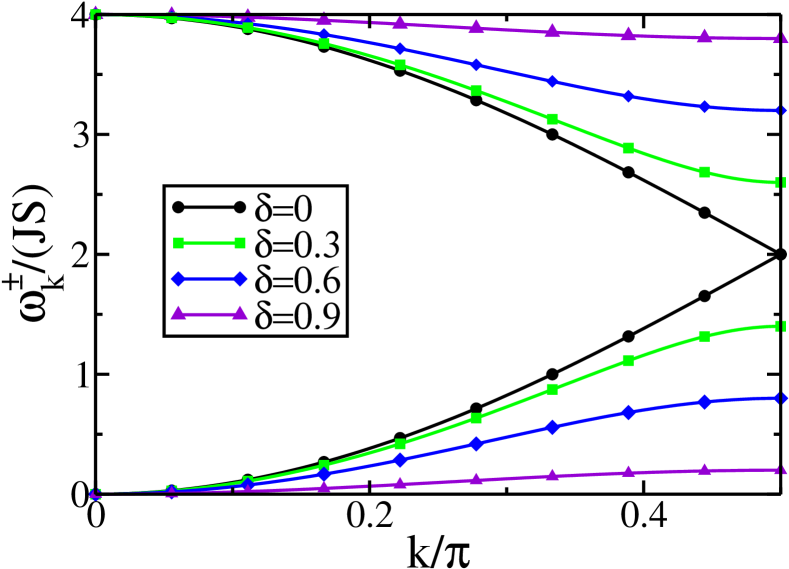
Figure 1: (Color online) Magnon dispersions obtained from MSWT for various dimerizations. The lower branches correspond to $\omega_{k}^{-}$ while the upper branches are given by $\omega_{k}^{+}$.

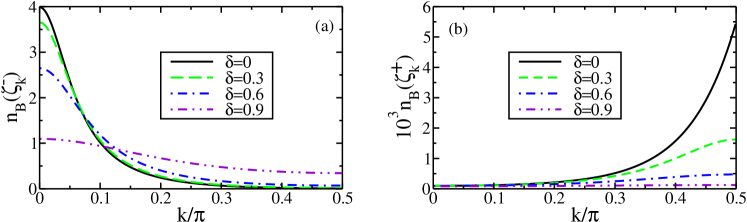
Figure 2: (Color online) Occupation numbers for the (a) lower and (b) upper branch for $S=1$ and $T=0.5J$ and various dimerizations as indicated.

Here $E_{S}^{0}=-JNS^{2}$ is the ground state energy at zero temperature ($T=0$), which is independent of the dimerization $\delta$, $k$ is the 1D momentum, and $\omega_{k}^{\pm}$ stands for the dispersion of the two magnon branches given by

$$\omega_{k}^{\pm}=2JS\left(1\pm\sqrt{\cos^{2}k+\delta^{2}\sin^{2}k}\,\right)\,.$$ (4)

From this expression it becomes clear that a finite dimerization, $\delta>0$, induces a splitting of the spin-wave dispersion into an accoustic and an optical branch at the boundaries $k=\pm\pi/2$ of the Brillouin zone. As a consequence, the two branches flatten with increasing dimerization. This is shown in Fig. 1 where the dispersions for various values of $\delta$ are shown.

To fulfill the Mermin-Wagner theorem of vanishing magnetization at finite temperature $T$, usual spin-wave theory has to be modified by a Lagrange multiplier serving as a chemical potential $\mu_{\delta}(T)$ that sets the finite temperature magnetization to zero.Takahashi (1987a, 1986) This results in the constraint

$$S=\frac{1}{N}\sum_{k}\{n_{\textnormal{B}}(\zeta_{k}^{-})+n_{\textnormal{B}}(\zeta_{k}^{+})\}\,.$$ (5)

Here

$$n_{\textnormal{B}}(x)=\frac{1}{\exp(\beta x)-1}$$ (6)

is the Bose distribution function, $\beta=1/T$, and

$$\zeta_{k}^{\pm}=\omega_{k}^{\pm}-\mu_{\delta}(T)$$ (7)

is the reduced magnon dispersion. The chemical potential $\mu_{\delta}(T)$ will be negative and vanishes as $T\rightarrow 0$.

Results obtained from this procedure are in excellent agreement with the Bethe ansatz results for the $S=1/2$ uniform ferromagnetTakahashi (1987a) ($\delta=0$) if $t_{\delta}/S\leq 1$, where we have defined a reduced temperature

$$t_{\delta}\equiv\frac{T}{JS(1-\delta^{2})}.$$ (8)

The occupation numbers for the lower and upper branch $n_{\text{B}}(\zeta_{k}^{-})$ and $n_{\text{B}}(\zeta_{k}^{+})$ are shown in Fig. 2 for $T/J=0.5$ and $S=1$. As expected, the occupation for the lower branch shows a maximum at $k=0$ whereas the occupation for the upper branch has a maximum at $k=\pi/2$. With increasing dimerization these peaks become less pronounced due to the flattening of the dispersions, see Fig. 1.

III Correlation functions

To obtain the spin correlation function (SCF) for an arbitrary distance $|i-j|$ it is crucial to include also the quartic terms in the bosonic operators stemming from the Dyson-Maleev transformation of the scalar product ${\bf S}_{i}\cdot{\bf S}_{j}$. This leads to

$$\langle{\bf S}_{i}{\bf S}_{j}\rangle=\left\{\begin{array}[]{rl}&S(S+1)\mbox{ for }i=j\\ &\frac{1}{4}\Big{(}\langle a_{i}^{\dagger}a_{j}\rangle+\langle a_{j}^{\dagger}a_{i}\rangle\Big{)}^{2}\mbox{ for }i\neq j\end{array}\right..$$ (9)

For $T>0$ the correlation function approaches zero in the limit $|i-j|\rightarrow\infty$ as $\langle a_{i}^{\dagger}a_{j}\rangle$ vanishes in this case.

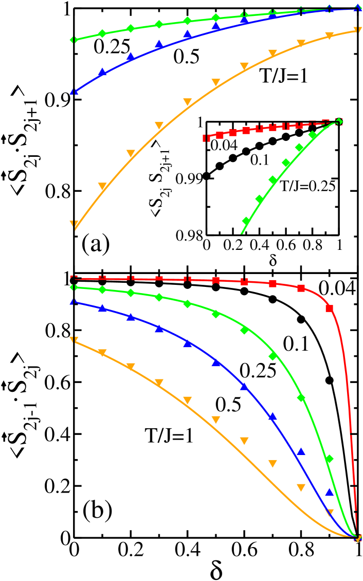
Figure 3: (Color online) Nearest neighbor spin correlation functions on (a) the strong bonds and (b) the weak bonds as a function of dimerization for various temperatures and $S=1$. The solid lines show the MSWT results. For comparison, TMRG data are shown as symbols. The inset shows data for low temperatures.

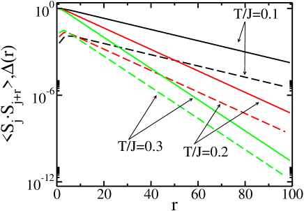
Figure 4: (Color online) Spin correlation function (solid lines) and alternation correlation function $\Delta(r)$ (dashed lines) for $S=1$ and $\delta=0.1$ and various temperatures as a function of distance $r$ obtained by MSWT. For a given temperature, the exponential decay of both quantities is determined by the same correlation length.

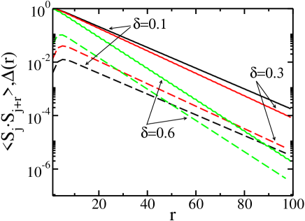
Figure 5: (Color online) Spin correlation function (solid lines) and alternation correlation function (dashed lines) obtained by MSWT for $S=1$ and $T/J=0.1$ and various dimerizations as indicated.

For the dimerized chain we obtain from Eq. (9)

$$\left<\boldsymbol{S}_{j}\cdot\boldsymbol{S}_{j+r}\right>=\left(\frac{1}{N}\sum_{k}\left[n_{\textnormal{B}}(\zeta^{-}_{k})+n_{\textnormal{B}}(\zeta_{k}^{+})\right]\cos(kr)\right)^{2},$$ (10)

if $r\neq 0$ is even, and

$$\left<\boldsymbol{S}_{j}\cdot\boldsymbol{S}_{j+r}\right>=\left(\frac{1}{N}\sum_{k}\left[n_{\textnormal{B}}(\zeta^{-}_{k})-n_{\textnormal{B}}(\zeta_{k}^{+})\right]f_{k}(j,r,\delta)\right)^{2},$$ (11)

if $r$ is odd. Here we have defined

$$f_{k}(j,r,\delta)\equiv\frac{\cos(kr)\cos k+(-1)^{j}\delta\sin(kr)\sin k}{\sqrt{\cos^{2}k+\delta^{2}\sin^{2}k}}.$$ (12)

Note that the summation in Eqs. (10) and (11) runs over the reduced Brillouin zone which is the reason for the minus sign in Eq. (11). From these expressions we obtain the nearest neighbor SCF shown in Fig. 3. One finds that the correlations on the strong bonds are enhanced while those on the weak bonds are reduced when the dimerization is increased. The dimerization strongly affects the SCF on the weak bonds whereas the strong bonds are far less affected. We find excellent agreement between the results obtained by MSWT and TMRG data up to $T/J=1$ and even the value at full dimerization ($\delta=1$) is captured correctly. However, MSWT suggests a quadratic behavior in $\epsilon\equiv 1-\delta$ on the weak bonds for $\epsilon\ll 1$ whereas a perturbative treatment starting from decoupled dimers shows a linear behavior as confirmed by the TMRG data. Finally the steep decrease of the nearest neighbor SCF on the weak bonds for low temperatures and strong dimerization indicates a non-analyticity for $T=0$ at $\delta=1$. Thus the ground state of the dimerized chain is always a uniform ferromagnetic state except for $\delta=1$ where it consists of decoupled dimers.

Next we shall explore the long-distance behavior of the spin-correlation function $\left<\boldsymbol{S}_{j}\cdot\boldsymbol{S}_{j+r}\right>$ and its variation with dimerization $\delta$ and temperature. In addition we define an alternation correlation function (ACF) for odd $r$ as

$$\Delta(r)\equiv|\left<\boldsymbol{S}_{j}\cdot\boldsymbol{S}_{j+r}\right>-\left<\boldsymbol{S}_{j}\cdot\boldsymbol{S}_{j-r}\right>|.$$ (13)

This expression describes the alternation of the SCF between the weak and the strong bonds and is thus a measure for the dimerization of the system. We exclude even $r$ in Eq. (13), as in this case $\Delta(r)=0$ by symmetry. In Fig. 5 the SCF and the ACF obtained from MSWT for $S=1$ and $\delta=0.1$ are shown for different temperatures and in Fig. 5 for $S=1$ and $T/J=0.1$ and different dimerizations. The asymptotic behavior of the correlation functions is governed in both cases by an exponential decay $\sim\text{e}^{-|r|/\xi_{\delta}}$ with the same correlation length $\xi_{\delta}$. As expected, increasing dimerization $\delta$ reduces the correlation length. For large dimerization the alternation of the exchange integrals leads to a staircase-like behavior of the SCF $\left<\boldsymbol{S}_{j}\cdot\boldsymbol{S}_{j+r}\right>$ (see Fig. 5 for $\delta=0.6$).

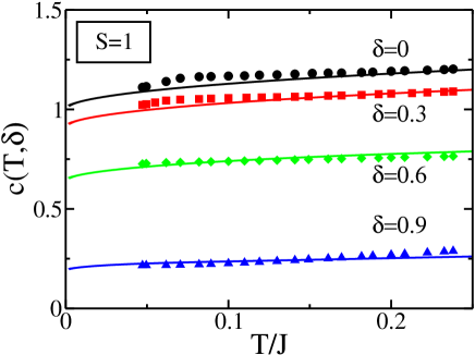
Figure 6: (Color online) Comparison of the function $c(T,\delta)$ as given by Eq. (17) (lines) and TMRG data (symbols) for $S=1$ and various $\delta$ as indicated.

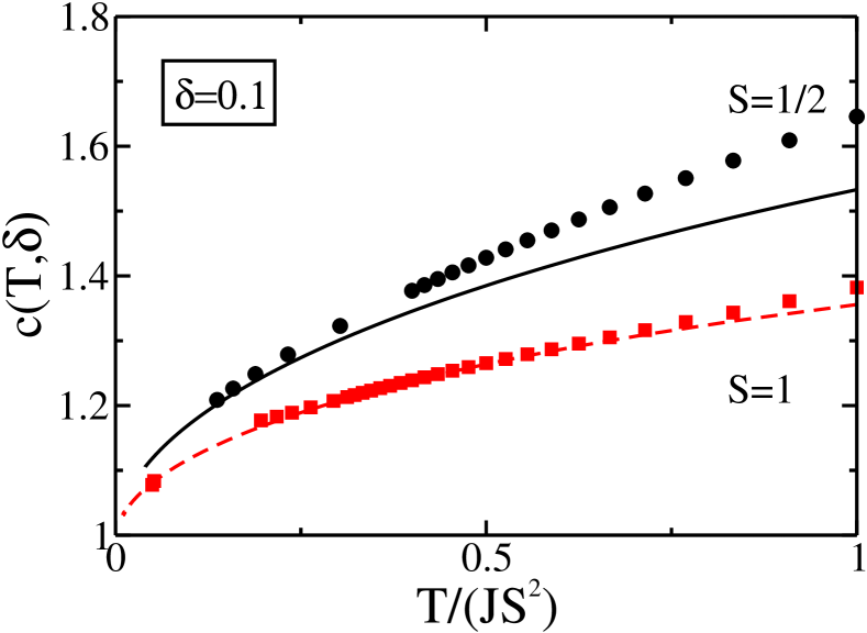
Figure 7: (Color online) Comparison of $c(T,\delta)$ for $S=1/2$ and $S=1$ as a function of temperature at $\delta=0.1$. The MSWT results (lines) are compared with TMRG data (circles and squares).

The function $c(T,\delta)$ (see Eq. (1)) describes the behavior of the correlation length as a function of dimerization and also gives corrections to the leading order $1/T$ temperature dependence. For a uniform 1D ferromagnet to lowest order in $T$ we have $c(T,\delta=0)=1$.Takahashi (1986) In order to go beyond this limit we have to investigate in detail the behavior of the SCF at large distances. For sufficiently low temperatures we may neglect contributions stemming from $n_{\textnormal{B}}(\zeta_{k}^{+})$ in Eqs. (5), (10), and (11). Expanding $\omega_{k}^{-}$ and $f_{k}(j,r,\delta)$ to lowest non-vanishing order and using a saddle point integration in Eqs. (10) and (11) we obtain in a large-$r$ expansion ($r\gg 1$)

$$\left<\mathbf{S}_{j}\cdot\mathbf{S}_{j+r}\right>\approx \frac{t_{\delta}}{4}\left(\frac{1}{\sqrt{v_{\delta}}}+\text{sgn}(r)\frac{(-1)^{j}(1-(-1)^{r})}{2}\delta\sqrt{t_{\delta}}\right)^{2}$$ (14)

$$\times\textnormal{e}^{-|r|/\xi_{\delta}},$$

with the correlation length

$$\xi_{\delta}=\frac{1}{2\sqrt{v_{\delta}t_{\delta}}}.$$ (15)

Here $v_{\delta}=-\mu_{\delta}/T$ is the negative reduced chemical potential reading

$$v_{\delta}=\frac{t_{\delta}}{4S^{2}}\left(1+\alpha\sqrt{t_{\delta}}+\frac{3}{4}\alpha^{2}t_{\delta}+\frac{\alpha^{3}}{2}t_{\delta}^{3/2}+\dots\right),$$ (16)

with $\alpha\equiv\zeta(\frac{1}{2})/(S\sqrt{\pi})$ where $\zeta(z)$ is Riemann’s zeta function. Eq. (14) explains why the SCF and the ACF both decay with the same correlation length. We note that for $\delta=0$ this expression agrees with the one obtained for the uniform case.Sirker and Bortz (2006)

	$\delta$ $a_{1}$ $a_{2}$ $a_{3}$ $a_{4}$
$S=\frac{1}{2}$	0 1.00000 1.16519 4.60822 9.66505 0.3 0.91000 1.11152 5.06398 11.1338 0.6 0.64000 0.93216 7.20035 18.8771 0.9 0.19000 0.50710 24.2538 116.701
$S=1$	0 1.00000 0.41195 0.07200 0.05339 0.3 0.91000 0.39298 0.07912 0.06151 0.6 0.64000 0.32956 0.11251 0.10428 0.9 0.19000 0.17956 0.37897 0.64469

Table 1: Coefficients of $c(T,\delta)$ given in Eq. (18) as extracted from Eq. (17) for $S=1/2$ and $S=1$. The coefficient $a_{1}$ is given by ($1-\delta^{2}$).

Figure 8: (Color online) (a) Spin correlation function $\left<\boldsymbol{S}_{j}\cdot\boldsymbol{S}_{j+r}\right>$ on a logarithmic scale for $S=1$, $T/J=0.1$ and $\delta=0.3$ obtained by TMRG compared with the analytical results from the asymptotic expansion, Eq. (14), and the short-range expression, Eq. (19), up to $r=4$. The solid line connects data obtained from a numerical solution of the MSWT, Eqs. (10) and (11), for integer $r$. (b) Same as above on a linear scale.

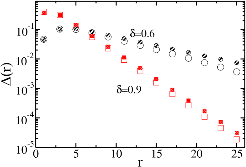
Figure 9: (Color online) Difference between the spin correlations on weak and strong bonds, see Eq. (13), for $S=1$, $T/J=0.1$, and two representative dimerization parameters. The filled symbols are data obtained from TMRG whereas the open symbols show results obtained by MSWT.

Inserting Eq. (16) into Eq. (15) and expanding for $t_{\delta}\ll 1$ we obtain the analytical expression

$$c(T,\delta)\approx(1-\delta^{2})\left(1-\frac{\alpha}{2}\sqrt{t_{\delta}}+\frac{5\alpha^{4}}{32}t_{\delta}^{2}-\frac{9\alpha^{5}}{64}t_{\delta}^{5/2}\right).$$ (17)

In Fig. 7, $c(T,\delta)$ for $S=1$ and various dimerizations is shown in comparison to numerical data from TMRG. We find excellent agreement between both methods. In Fig. 7, $c(T,\delta)$ is shown for $S=1/2$ and $S=1$ as a function of temperature for $\delta=0.1$. Note that $c(T,\delta)$ is much steeper for $S=1/2$, see Eq. (17). In Tab. 1 the coefficients $a_{1}$, $a_{2}$, $a_{3}$, and $a_{4}$ of the series

$$c(T,\delta)\approx a_{1}+a_{2}\sqrt{\frac{T}{J}}+a_{3}\left(\frac{T}{J}\right)^{2}+a_{4}\left(\frac{T}{J}\right)^{5/2}$$ (18)

are shown as extracted from Eq. (17). We remark that the higher order corrections $a_{3}$ and $a_{4}$ are much larger for $S=1/2$ than for $S=1$ and increase with increasing dimerization.

Apart from the large-$r$ expansion, an analytical expression for small distances can also be obtained from Eqs. (10) and (11). Again neglecting contributions stemming from $n_{\text{B}}(\zeta_{k}^{+})$ and expanding the dispersion as well as the function $f_{k}(j,r,\delta)$, Eq. (12), to second order in $k$ we find the short-distance expansion

$$\left<\boldsymbol{S}_{j}\cdot\boldsymbol{S}_{j+r}\right> \approx S\left\{S-\frac{t_{\delta}^{3/2}(\zeta(\frac{3}{2})-2\sqrt{\pi v_{\delta}}-\zeta(\frac{1}{2})v_{\delta})}{4\sqrt{\pi}}\right.$$ (19)

$$\left.\times\left[r^{2}+\delta\left((-1)^{r}-1\right)\left((-1)^{j}r-\frac{\delta}{2}\right)\right]\right\}.$$

In Fig. 8 the SCF is presented for $S=1$, $T/J=0.1$ and $\delta=0.3$ as a function of distance. Fig. 8(a) compares a numerical self-consistent solution of Eqs. (10) and (11) with the expansion for small distances $r$, Eq. (19), and the long distance asymptotics, Eq. (14). Furthermore, numerical TMRG data are shown. For $r\gg 1$ the exponential decay of the SCF, as derived from the MSWT is clearly visible. When applicable, we find good agreement between the analytical expressions for short and long distances and the results obtained by TMRG. The same quantities for the same parameters are shown in Fig. 8(b) on a linear scale. In Fig. 9 we compare the ACF for spin $S=1$ and two large values of the dimerization parameter, $\delta=0.6$ and $0.9$, as obtained from MSWT, with TMRG data. Although a high dimerization leads to a high effective temperature $t_{\delta}$ the agreement of the MSWT with the numerical data is still remarkably good.

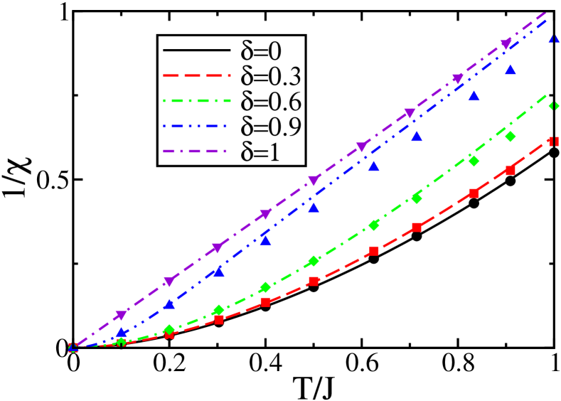
Figure 10: (Color online) Inverse susceptibility $1/\chi$ as a function of $T/J$ for $S=1$ and different values of $\delta$ as indicated. The lines show the results from MSWT, the symbols for $\delta<1$ TMRG data, and the symbols for $\delta=1$ the exact solution for decoupled dimers. An increasing dimerization suppresses $\chi$, and the decoupled dimers follow a Curie law $\chi\sim 1/T$.

Next, we calculate the zero field susceptibility per site

$$\chi=\frac{1}{3NT}\sum_{j,l}\left<\boldsymbol{S}_{j}\cdot\boldsymbol{S}_{l}\right>.$$ (20)

Applying the Dyson-Maleev transformation we find

$$\chi=\frac{S}{3T}+\frac{1}{6NT}\sum_{k}\left\{(n_{k}^{+})^{2}+(n_{k}^{-})^{2}\right\},$$ (21)

with

$$n_{k}^{\pm}\equiv n_{\text{B}}(\zeta_{k}^{-})\pm n_{\text{B}}(\zeta_{k}^{+}).$$

In order to obtain an analytical result for the susceptibility, we may interpolate the SCF in Eq. (20) between the short-range limit given in Eq. (19) and the asymptotic expression of Eq. (14). From this we obtain

$$\chi=\frac{2}{3}\frac{\xi_{\delta}S^{2}}{T} \left[1-\frac{3\zeta(\frac{1}{2})}{2\sqrt{\pi}S}\frac{1}{\sqrt{\xi_{\delta}}}-\frac{2\pi S\delta-3\zeta^{2}(\frac{1}{2})}{4\pi S^{2}}\frac{1}{\xi_{\delta}}+\dots\right],$$ (22)

where we have used that to lowest order the correlation length is given by $\xi_{\delta}=S/t_{\delta}$. In the limit of vanishing dimerization our result reduces to the result previously found by Takahashi for the uniform chain.Takahashi (1986); chi

In the opposite limit of full dimerization the susceptibility can easily be calculated exactly. In this case we have decoupled ferromagnetic dimers and the suceptibility follows a Curie law at low temperatures. Within MSWT we find from Eq. (21)

$$\chi(\delta=1)=\frac{S+2\{n^{2}_{\text{B}}(v_{1})+n^{2}_{\text{B}}(4JS+v_{1})\}}{3T}.$$ (23)

For $T/J\ll 1$ this expression reduces to

$$\chi\approx\frac{S(2S+1)}{3T},$$ (24)

which is the Curie law (per spin) for decoupled ferromagnetic dimers. In Fig. 10 the inverse susceptibility $1/\chi$ as obtained from MSWT is compared with TMRG data. The agreement is good for $t_{\delta}/S\leq 1$ and also the case of decoupled dimers is accurately captured by MSWT.

IV Dynamical spin structure factor

For the dimerized AF Heisenberg chain the dynamical spin structure factor (dynamic SSF) has been intensely studied by various methods.Uhrig and Schulz (1996); Poilblanc et al. (1997); Augier et al. (1997); Yu and Haas (2000) Here we will discuss the impact of a finite dimerization on the dynamic SSF of the FM Heisenberg chain. The dynamical properties of the uniform 1D ferromagnet within MSWT have been adressed by Takahashi.Takahashi (1990, 1993) In this case for a given value of $q$ the dynamic SSF exhibits a magnon peak from which the magnon dispersion can be obtained. In this approximation magnon-magnon interactions are not taken into account and the peaks are broadened due to thermal fluctuations only. The magnon peaks, which exhibit a Lorenzian lineshape at finite temperatures, thus reduce to $\delta$-functions at $T=0$. Moreover, there is a two-magnon continuum beyond which the dynamic SSF vanishes. New aspects to this picture have been added recentlyHerzog et al. (2011) when it was shown that an edge singularity occurs at the boundary of the two-magnon continuum caused by a diverging density of states.

Here we want to generalize this analysis to the dimerized FM chain. Within the standard approach of neutron scattering the differential cross-section is directly related to the dynamic SSF.Marshall and Lovesey (1971) The latter can be obtained by a Fourier transform of the two-point correlation function. It was shown in the context of X-ray scattering that further insight into the microscopic properties of physical systems may be achieved if the incident photon fulfills the Bragg condition such that the resulting state is given by a coherent superposition of the forward diffracted and the Bragg reflected wave.Schülke (1981, 1982, 2001) The structure factor can be written as a matrix in terms of the reciprocal lattice vectors in analogy to the dielectric matrix whose inverse defines the dynamic charge structure factor of a dielectric.Adler (1962); Wiser (1963); von der Linden and Horsch (1988)

In the same spirit we formulate the dynamic SSF of the dimerized FM chain as a $2\times 2$-matrix

$$\boldsymbol{S}(q,\omega)=\left(\begin{array}[]{cc}S(q,q,\omega)&S(q,q+\pi,\omega)\\ S(q+\pi,q,\omega)&S(q+\pi,q+\pi,\omega)\end{array}\right).$$

In order to obtain this matrix we calculate the Green’s function

$$G(j,r,\tau)\equiv-\left<\mathcal{T}\left[\boldsymbol{S}_{j}(0)\cdot\boldsymbol{S}_{j+r}(\tau)\right]\right>,$$ (25)

which within MSWT reads

$$G(j,r,\tau) =-\left<\mathcal{T}\left\{a^{\ }_{j}(0)a_{j+r}^{\dagger}(\tau)\right\}\right>$$ (26)

$$\times\left<\mathcal{T}\left\{a_{j}^{\dagger}(0)a^{\ }_{j+r}(\tau)\right\}\right>.$$

From this the matrix elements of the dynamic SSF can be obtained straightforwardly via

$$S(q,q^{\prime},\omega)=2n_{\text{B}}(-\omega)\text{Im}G^{\text{ret}}(q,q^{\prime},\omega),$$ (27)

where $G^{\text{ret}}(q,q^{\prime},\omega)$ is the retarded finite temperature Green’s function obtained from $G(j,r,\tau)$. For the diagonal elements we find $S(q,q,\omega)=S(q+\pi,q+\pi,\omega)$ with

$$S(q,q,\omega)= \frac{\pi}{N}n_{\text{B}}(-\omega)\sum_{\sigma,\sigma^{\prime}\in\{\pm\}}\sum_{k}\delta(\omega-\epsilon^{\sigma\sigma^{\prime}}_{q}(k))$$ (28)

$$\times\left\{1+\sigma\sigma^{\prime}\Phi(k,q+k)\right\}\mathcal{N}[\zeta_{k}^{\sigma},\zeta_{q+k}^{\sigma^{\prime}},\beta],$$

where we have defined

$$\Phi(k,k^{\prime})\equiv\frac{\cos k\cos k^{\prime}-\delta^{2}\sin k\sin k^{\prime}}{\sqrt{1-(1-\delta^{2})\sin^{2}k}\sqrt{1-(1-\delta^{2})\sin^{2}k^{\prime}}}.$$ (29)

and

$$\mathcal{N}[\zeta^{\sigma}_{k},\zeta^{\sigma^{\prime}}_{q+k},\beta]\equiv n_{\textnormal{B}}(\zeta_{k}^{\sigma})\{1+n_{\textnormal{B}}(\zeta_{q+k}^{\sigma^{\prime}})\}$$ (30)

$$\times\left(\textnormal{e}^{-\beta\epsilon_{q}^{\sigma\sigma^{\prime}}(k)}-1\right)\,,$$

with the two particle continuum $\epsilon_{q}^{\sigma\sigma^{\prime}}(k)\equiv\zeta_{k}^{\sigma}-\zeta_{q+k}^{\sigma^{\prime}}$. As in the case of the uniform 1D ferromagnet the dynamic SSF for the dimerized chain fulfills detailed balance.

Figure 11: (Color online) Diagonal elements of the dynamic spin structure factor $S(q,q,\omega)$ for a dimerized ferromagnetic chain and $S=1$, $T/J=0.1$: (a) $S(q,q,\omega)$ spectra for different momenta $q$ and $\delta=0.6$. The red dashed lines show the edge boundaries and the symbols show the peak positions projected onto the $(q,\omega)$-plane. (b) broadened spectra $I_{\Lambda}(q,q,\omega)$ for $q=4\pi/5$, $\delta=0.4$ and for different $\Lambda=0,0.001,0.01,$ and $0.1J$. Vertical lines in $\Lambda=0$ panel indicate positions of edge singularities.

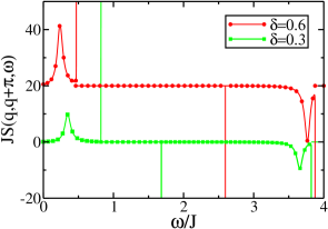
Figure 12: (Color online) Off-diagonal element of the dynamical spin structure factor matrix $S(q,q+\pi,\omega)$ for $q=\pi/5$, $S=1$, $T/J=0.1$, and $\delta$ as indicated. Note that the data for $\delta=0.6$ are shifted by 20 units along the ordinate for clarity of presentation. The vertical lines indicate positions of edge singularities (see text).

In this approximation the two magnon continuum determines the regions where $S(q,q,\omega)$ is nonzero. This can be seen in Fig. 11(a) where the diagonal element of the dynamic SSF for the dimerized chain is shown for $\delta=0.6$. The symbols reflect the peak positions projected onto the $(q,\omega)$-plane. They follow the reduced magnon dispersions $\zeta_{q}^{\pm}$. Since we are dealing with two separate magnon branches, an edge singularity occurs at each boundary of the two magnon continua due to the divergence of the respective density of states. The boundaries beyond which the dynamic SSF for the respective branch vanishes are given by the red dashed lines. For $\omega>0$ we find three boundaries out of the four possible combinations because for $\epsilon_{q}^{-+}$ the argument of the delta function in Eq. (28) never vanishes.

Experimentally, the energy resolution in a measurement is always finite. An important question to ask is therefore if the edge singularities can be resolved at all. We address this question by studying the dynamical SSF with a finite energy resolution $\Lambda$

$$I_{\Lambda}(q,q,\omega)=\frac{1}{2\Lambda}\int\limits_{\omega-\Lambda}^{\omega+\Lambda}d\omega_{0}\ S(q,q,\omega_{0}).$$

Results for this quantity are shown in Fig. 11(b) for $\delta=0.4$ and various resolutions. Being very close to a magnon peak, the lower edge singularity has a substantial spectral weight. Even with a relatively moderate energy resolution this edge singularity is therefore detectable. On the contrary, the two edge singularities at higher energies carry almost no spectral weight in the considered example making them experimentally irrelevant.

The off-diagonal elements of the dynamic SSF, $S(q,q+\pi,\omega)=S(q+\pi,q,\omega)$, are given by

$$S(q,q+\pi,\omega)= \frac{\pi}{N}n_{\text{B}}(-\omega)\sum_{\sigma,\sigma^{\prime}\in\{\pm\}}\sum_{k}\delta(\omega-\epsilon^{\sigma\sigma^{\prime}}_{q}(k))$$ (31)

$$\times\sigma\sigma^{\prime}\Psi(k,q+k)\mathcal{N}[\zeta_{k}^{\sigma},\zeta_{q+k}^{\sigma^{\prime}},\beta],$$

where we have defined

$$\Psi(k,k^{\prime})=\frac{2\delta\cos k\sin k^{\prime}}{\sqrt{1-(1-\delta^{2})\sin^{2}k}\sqrt{1-(1-\delta^{2})\sin^{2}k^{\prime}}}.$$ (32)

Examples for the off-diagonal element of the dynamic SSF matrix are shown in Fig. 12. As in the case of $S(q,q,\omega)$ the two-magnon continuum determines the region where $S(q,q+\pi,\omega)\neq 0$ with edge singularities at the boundaries. Moreover we find magnon peaks of different signs following the magnon dispersions.

V Static spin-structure factor

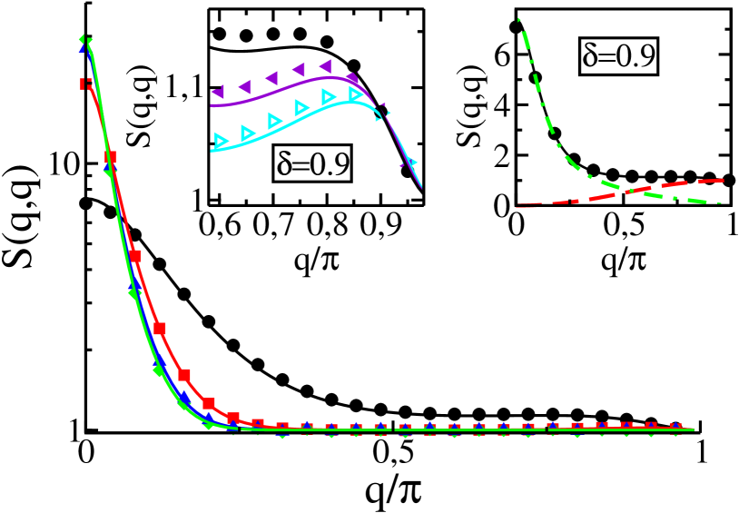
Figure 13: (Color online) Diagonal static spin structure factor for $S=1$, $T/J=0.1$. Symbols denote data from TMRG, lines results from MSWT. Main: Data for dimerizations $\delta=0$ (diamonds), $\delta=0.3$ (triangles), $\delta=0.6$ (squares), and $\delta=0.9$ (circles). Left inset: High-momentum peak for $\delta=0.9$ at $T/J=0.1$ (circles), $T/J=0.08$ (filled triangles), and $T/J=0.0625$ (open triangles). Right inset: Data for $\delta=0.9$ with contributions stemming from the lower and upper branch shown by dashed-dotted and dashed lines, respectively.

The static spin structure factor (static SSF) matrix can be easily obtained from the dynamic SSF via

$$S(q,q^{\prime})=\int\limits_{-\infty}^{\infty}\frac{d\omega}{2\pi}S(q,q^{\prime},\omega).$$ (33)

We first want to discuss the diagonal elements of this matrix. We divide $S(q,q)=S^{-}(q,q)+S^{+}(q,q)$ with $S^{-}(q,q)$ ($S^{+}(q,q)$) being the part which stems from the lower (upper) branch of the dispersion. These contributions are given by Eqs. (28) with $\sigma=\sigma^{\prime}$ and $\sigma\neq\sigma^{\prime}$ (see also Fig. 11). Performing the frequency integrals we find

$$S^{-}(q,q)=\frac{1}{2N} \sum_{\sigma\in\{\pm\}}\sum_{k}\left[1+\Phi(k,q+k)\right]n_{\text{B}}(\zeta^{\sigma}_{k})$$ (34)

$$\times\left[1+n_{\text{B}}(\zeta_{q+k}^{\sigma})\right],$$

and

$$S^{+}(q,q)=\frac{1}{2N} \sum_{\sigma\in\{\pm\}}\sum_{k}\left[1+\Phi(k,q+k)\right]n_{\text{B}}(\zeta^{\sigma}_{k})$$ (35)

$$\times\left[1+n_{\text{B}}(\zeta_{q+k}^{-\sigma})\right].$$

From this we have

$$S(q,q)=\frac{1}{2N}\sum_{k}\Biggl{\{}n_{k}^{+}n_{q+k}^{+}+n_{k}^{-}n_{q+k}^{-}\Phi(k,q+k)\Biggr{\}}+S.$$ (36)

Alternatively, the diagonal elements of the static SSF can be obtained directly from

$$S(q,q)=\frac{1}{N}\sum_{j,l}\left<\boldsymbol{S}_{j}\cdot\boldsymbol{S}_{l}\right>\text{e}^{iq(j-l)}.$$ (37)

However, within the latter approach the distinction of the contributions stemming from the lower and the upper branch of the dynamic SSF is less transparent.

In Fig. 13 the diagonal structure factor $S(q,q)$ is shown for various dimerizations at $T/J=0.1$ with $S=1$. The agreement between the MSWT results and the numerical TMRG data is good even for high dimerizations. An increasing dimerization leads to an increase of the linewidth of the central peak at $q=0$. At high dimerizations a shoulder in $S(q,q)$ appears that extends almost up to $q=\pi$. At low temperatures a second maximum develops near $q=\pi$ (see left inset of Fig. 13). For decreasing temperatures the peak shifts to higher momenta leading to a sharp maximum close to the boundary of the Brillouin zone for very low temperatures and high dimerizations.

For a dimerized FM chain with $\delta<1$ such a high momentum structure is expected due to the commensurate modulation of the exchange constant.rem (a) The naive expectation of a peak right at $\pi$ indicating the dimerization of correlation functions is, however, not fulfilled. Instead, we find a small peak with momentum shifted away from $q=\pi$. This can be readily understood by considering $S^{-}(q,q)$ and $S^{+}(q,q)$ separately as is done in the right inset of Fig. 13. $S^{-}(q,q)$ is peaked at $q=0$ and $S^{+}(q,q)$ reveals a maximum at $q=\pi$. However, at sufficiently high dimerizations the $S^{-}(q,q)$ contribution also yields a significant contribution for $q\geq\pi/2$. Therefore the two contributions add up to a peak which is shifted with respect to $q=\pi$.

One may also wonder why the dimerization does not show up more pronounced in the diagonal elements of the static spin structure factor matrix, i.e., why the peak at $q=0$ has much more weight than the high momentum peak even at strong dimerizations. To investigate this property, we insert Eq. (14) into Eq. (37) dividing the SCF into a uniform and an alternating part. Performing the sum over $r$ to lowest order we end up with

$$S(q,q)\approx\frac{1}{\xi_{\delta}}\left\{\frac{A}{q^{2}+\xi_{\delta}^{-2}}+\frac{B}{(q-\pi)^{2}+\xi^{-2}_{\delta}}\right\},$$ (38)

with

$$A=\frac{t_{\delta}}{4}\left(\frac{1}{v_{\delta}}+\delta^{2}t_{\delta}\right)$$

and

$$B=\frac{t_{\delta}^{2}\delta^{2}}{4}.$$

Thus, as expected, we find two Lorentzians at $q=0$ and $q=\pi$, respectively. However, the ratio

$$\frac{S(\pi,\pi)}{S(0,0)}=\frac{v_{\delta}t_{\delta}\delta^{2}}{1+v_{\delta}t_{\delta}\delta^{2}}$$ (39)

is small for effective temperatures $t_{\delta}\ll 1$. For large $t_{\delta}$, on the other hand, we have $\xi_{\delta}\ll 1$ and the two Lorentzians become very broad.

Finally, from the left inset of Fig. 13 we see that the peak position of the maximum at high momentum is temperature dependent. On the other hand, we find that for $t_{\delta}$ and $S$ fixed the peak position does not depend on $\delta$. To understand this puzzling feature we derive an analytical expression for the position of the high momentum peak. Keeping only contributions from $n_{\text{B}}(\zeta_{k}^{-})$ in Eq. (36), expanding $\Phi(q,k)$ around $q=\pi$ and $k=0$, and performing a saddle-point integration we can evaluate the remaining expression. Using Eq. (16) we find that the high-momentum peak is located at

$$q_{\text{max}}=\pi-\sqrt[4]{\frac{2}{S^{2}}}t_{\delta}^{3/4}+\frac{1}{2}\frac{t_{\delta}^{5/4}}{\sqrt[4]{8S^{6}}}+\dots$$ (40)

which explains why the peak position does not depend explicitly on $\delta$.

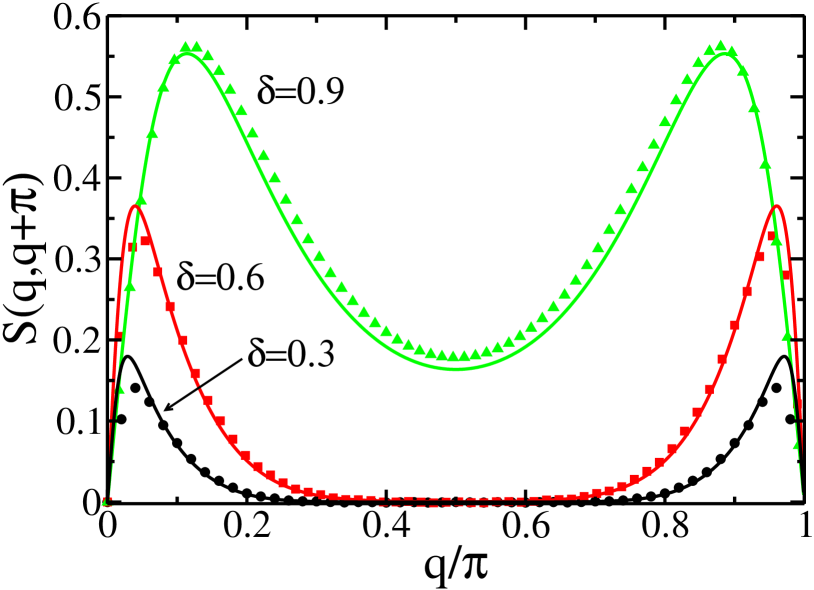
Figure 14: (Color online) Off-diagonal elements of the static spin structure factor matrix for $S=1$, $T/J=0.1$, and various dimerizations as a function of $q$. The symbols show numerical data obtained by TMRG, whereas the solid lines are results from MSWT, Eq. (41).

Next, we turn to the off-diagonal elements of the static SSF matrix. From integrating Eq. (31) over frequency we find

$$S(q,q+\pi)=\frac{1}{2N}\sum_{k}\Psi(k,q+k)n_{k}^{-}n_{q+k}^{-}.$$ (41)

The off-diagonal elements vanish in the undimerized case and are finite in the dimerized case. Thus they provide a rigorous criterion for dimerized spin correlation functions. In Fig. 14 this expression is shown for $S=1$, $T/J=0.1$, and various dimerizations. $S(q,q+\pi)$ is an odd function of momentum transfer $q$, and is a symmetric function with respect to $q=\pi/2$. It exhibits a two peak structure which is more pronounced the higher the dimerization is. In complete analogy to the high-momentum peak of $S(q,q)$ we can again determine the positions of the maxima of $S(q,q+\pi)$ and find

$$q_{\text{max}}=\frac{\pi}{2}\pm\left(\frac{1}{\xi_{\delta}}-\frac{\pi}{2}\right).$$ (42)

Hence, as in the previous case, the peak positions of $S(q,q+\pi)$ are determined by the spin quantum number $S$ and the reduced temperature $t_{\delta}$ only. In particluar we observe that the distance from the center (boundary) of the Brillouin zone of the low (high) momentum peak is given by the inverse correlation length $\xi_{\delta}^{-1}$.

To summarize, dimerization is signaled by the appearance of finite intensity in the off-diagonal spin structure factor. On the other hand, the conventional (diagonal) structure factor reflects the FM spin-Peierls dimerization mainly by quantitative changes, in particular by an increase of the linewidth of the $q=0$ peak. As a qualitative change, a high-momentum maximum at large dimerizations and low-temperatures develops in the diagonal structure factor, however, this structure always has a very small intensity.

VI Conclusions

We have shown that an alternation of the magnetic exchange can also occur in ferromagnetic spin chains. Possible mechanisms are a coupling to orbital fluctuations, as in YVO₃Ulrich et al. (2003); Sirker and Khaliullin (2003); Sirker et al. (2008), or to lattice degrees of freedom. In both cases the dimerization has to be thermally activated leading to a gain in magnetic energy $\sim-T^{3/2}\delta^{2}$. In an adiabatic approximation the loss in potential energy is $\sim K\delta^{2}$ where $K$ is an effective elastic constant. A dimerized phase due to coupling to the lattice is therefore only possible as a finite-temperature phase and only if $K$ is smaller than some threshold value.

As an analytical method to calculate the thermodynamic properties of a dimerized ferromagnetic Heisenberg chain we have used a modified spin-wave theory. By comparing with numerical data obtained by the transfer matrix renormalization group, we have shown —as a central result of this paper—that the modified spin-wave theory yields excellent results for a wide range of dimerization parameters and temperatures.

We found that both the spin and the dimer correlation functions decay exponentially at finite temperatures with the same correlation length $\xi_{\delta}=c(T,\delta)JS^{2}/T$. The correlation length $\xi_{\delta}$ decreases with increasing dimerization $\delta$. Next-leading corrections to the $1/T$ behavior have been calculated explicitly for spin $S=1/2$ and $S=1$ and even these corrections (of order 1) described by the coefficient $c(T,\delta)$ have been shown to be in excellent agreement with the numerical data. For dimerizations $\delta<1$ the magnetic susceptibility diverges as $\chi\sim(1-\delta^{2})/T^{2}$, i.e., the susceptibility at low temperatures is suppressed with increasing dimerization. For $\delta=1$ we have a system of decoupled dimers and $\chi\sim 1/T$.

Similarly to X-ray scattering experiments, where the incident photon is given by a coherent superposition of the forward diffracted and the Bragg reflected wave, we have formulated the dynamic spin stucture factor for neutron scattering experiments as a matrix. The diagonal elements correspond to the standard dynamic spin structure factor while the off-diagonal elements include a reciprocal lattice vector. The dimerization leads to two magnetic excitation branches which are clearly visible in the diagonal elements of the dynamic spin structure factor matrix. Within the spin-wave approximation used here, this quantity is zero outside the two-magnon continuum. At the boundary of the two-magnon continuum edge singularities are formed due to a diverging density of states. These singularities might become smooth once higher magnon excitations are included but we expect that a peak-structure remains along the two-magnon boundary. Experimentally, the edge singularities can only be resolved if they carry sufficient spectral weight. This is only the case if they occur close to a magnon peak. For the off-diagonal elements of the dynamic spin structure factor matrix we also find magnon peaks with different signs for the upper and lower magnon branch. The two-magnon continuum determines the region where the off-diagonal elements of the dynamic spin structure factor is nonzero with edge singularities occuring at the boundaries.

The diagonal elements of the static spin structure factor matrix exhibit $q=0$ peaks with Lorentzian lineshape. The linewidth of the latter increases with increasing dimerization. Furthermore, for strong dimerizations a high momentum peak is observed. We find that the position of the peak at high momenta depends solely on $S$ and the reduced temperature $t_{\delta}=T/(JS(1-\delta^{2}))$. The dimerization leads to a doubling of the unit cell which manifests itself by the appearance of a finite off-diagonal structure factor. The off-diagonal elements of the static spin structure factor matrix show a two-peak structure which becomes more pronounced the higher the dimerization is. The distance of the maxima with respect to the center and boundary of the Brillouin zone are given by the inverse correlation length.

To conclude, a spin-Peierls state can be realized in ferromagnetic spin chains but only at finite temperatures. Most promising candidates for this new state are, as we have argued, monatomic chains on surfaces where the effective elastic constants are expected to be rather small.