Theoretical description of two ultracold atoms in finite 3D optical lattices using realistic interatomic interaction potentials

Abstract

A theoretical approach is described for an exact numerical treatment of a pair of ultracold atoms interacting via a central potential that are trapped in a finite three-dimensional optical lattice. The coupling of center-of-mass and relative-motion coordinates is treated using an exact diagonalization (configuration-interaction) approach. The orthorhombic symmetry of an optical lattice with three different but orthogonal lattice vectors is explicitly considered as is the Fermionic or Bosonic symmetry in the case of indistinguishable particles.

I Introduction

The physics of ultracold quantum gases attracts a lot of interest since the experimental observation of Bose-Einstein condensation in dilute alkali-metal atom gases Anderson et al. (1995); Davis et al. (1995). Besides the exciting physics of ultracold gases by itself, a further important progress was the loading of the ultracold gas into an optical lattice formed with the aid of standing light waves Jaksch et al. (1998); Greiner et al. (2002); Köhl et al. (2005). The optical lattice resembles in some sense the periodicity of a crystal potential Meacher (1998); Bloch (2005); Lewenstein et al. (2007); Bloch et al. (2008), but is practically free of phonons. In contrast to real solids the lattice parameters are, in addition, easily tunable by a variation of the laser intensity, the relative orientation of the laser beams, or the wavelength. In the first case the lattice depth, in the other cases the lattice geometry can be manipulated.

Moreover, in the ultracold regime the effective long-range interaction between atoms is usually well characterized by a single parameter, the scattering length Weiner et al. (1999). This simplifies the investigation of atomic systems in the ultracold regime. The effective interaction can be either attractive or repulsive, depending on the type of atoms involved. While different kinds of chemical elements, their isotopes, or atoms in different electronic or spin states cover already a wide range of interaction strengths, an almost full tunability of the atom-atom interactions in ultracold gases is achieved using magnetic Feshbach resonances Loftus et al. (2002); Regal et al. (2003). Close to the resonance value of the magnetic field the scattering length diverges and the effective interaction varies in a wide range, in principle from being infinitely strongly repulsive to infinitely strongly attractive. This possibility of active control of the interparticle interaction makes ultracold atoms in optical lattices an ideal tool for, e. g., exploring the properties of many-body Hamiltonians describing particles in periodic potentials, like the Hubbard model Hubbard (1963); Jaksch et al. (1998). Examples are the experimental studies of a Bosonic Mott insulator Greiner et al. (2002), a Fermionic band insulator Köhl et al. (2005), or the simulation of antiferromagnetic spin chains in an optical lattice Simon et al. (2011).

A further important aspect of ultracold quantum gases in optical lattices is the in principle arbitrary filling that can be realized, while the filling is strongly constrained in usual solid-state systems by charge neutrality. Ultracold quantum gases thus allow studies far away from the often considered half-filling case. One interesting limit is the one of very sparsely populated lattices in which few-body quantum dynamics can be studied very accurately Kraemer et al. (2006). This initiated recently a number of corresponding theoretical studies Valiente et al. (2010a, b); Chatterjee et al. (2010). These investigations are often further motivated by the fact that the direct experimental control of many parameters together with the high degree of coherence that is not destroyed by phonons led to proposals to use ultracold quantum gases in optical lattices in quantum-information applications like quantum simulators or even quantum computers DeMille (2002); Jaksch and Zoller (2004); Lewenstein et al. (2007); Bloch et al. (2008); Simon et al. (2011); Schneider and Saenz (2011). For such applications a very precise knowledge about the microscopic interactions between quantum particles in an optical lattice is a prerequisite.

At the required level of accuracy a description of the atoms as simply being trapped in an array of harmonic potentials becomes inappropriate. For example, during a controlled quantum-gate operation it is usually necessary to bring two atoms from different sites into contact with each other. Atoms in different electronic states may be involved in such an operation, as those states may encode the two qubit states ($|0\rangle$ and $|1\rangle$). However, in such a case the center-of-mass (c.m.) and relative (rel.) motions of two atoms even in the same potential well do not separate, even not within the harmonic approximation Bolda et al. (2005); Grishkevich and Saenz (2007). This is due to the fact that different hyperfine states are usually accompanied by different polarizabilites. Thus the atoms in different states experience different trapping frequencies even within the harmonic approximation. Evidently, such a non-separability of c.m. and rel. motions always occurs for heteronuclear systems (different atomic species) with different masses and polarizabilites. Experimental evidence for the corresponding breakdown of the harmonic approximation for a heteronuclear system was given in Ospelkaus et al. (2006) and theoretically confirmed Deuretzbacher et al. (2008); Grishkevich and Saenz (2009). If the considered atoms are not tightly bound in the same potential well and thus if the multi-well structure of the optical lattice is important, there is evidently no separability of c.m. and rel. motion, even not for identical atoms.

Already the theoretical treatment of two atoms in an optical lattice is a formidable task, if realistic atom-atom interaction needs to be considered. While this interaction may often be described by a central force, the interaction potential stems from laborious quantum-chemistry calculations and is thus only numerically given. The transition to c.m. and rel. coordinates simplifies the problem dramatically, since the interatomic interaction affects only the rel. motion and in the case of an isotropic interaction even only the radial part of it. However, the above-mentioned non-separability demands finally to treat the full six-dimensional problem. Furthermore, the matrix elements describing the interaction with the trapping potential become more involved, since they do not separate in c.m. and rel. coordinates. Alternatively, the problem may be solved in (absolute) Cartesian coordinates. In this case the potential describing the optical lattice separates for both particles and, e. g., in the orthorhombic case even for the three Cartesian coordinates. However, in this case the particle interaction terms restore the non-separability of the six-dimensional problem, except for very special cases like the $r^{2n}$ potentials Armstrong et al. (2011) where $r$ is the radial coordinate of rel. motion and $n$ is an integer. In view of its universality with respect to the interparticle interaction the treatment in c.m. and rel. coordinates is favorable. Furthermore, as will be shown in detail below, the use of Taylor expansions of the optical-lattice potential allows for a reasonable efficiency.

In this work a numerical approach is presented for the theoretical treatment of two particles that interact via a central (isotropic) interaction potential and are trapped in a finite orthorhombic $\sin^{2}$- or $\cos^{2}$-type periodic potential. While the main motivation is the treatment of ultracold atoms and molecules in optical lattices, the code allows also to treat other particles and was, e. g., recently also employed in a study of electrons and excitons in quantum-dot molecules. The uncoupled Schrödinger equations for c.m. and rel. motion are solved by an expansion of the radial parts in $B$ splines and the angular parts in spherical harmonics. The coupling is then considered by means of configuration interaction (exact diagonalization). The orthorhombic D_2h symmetry is fully accounted for.

The approach was already successfully applied in a systematic investigation of the effects of anharmonicity and coupling of c.m. and rel. motion for two atoms in a single well of an optical lattice Grishkevich and Saenz (2009). Together with the experimental results in Ospelkaus et al. (2006) this allowed the conclusion that only the inclusion of the effects of anharmonicity and coupling (and thus deviations from a simple uncoupled harmonic model) lead to agreement with experiment. Furthermore, considering a triple-well potential the optimal Bose-Hubbard parameter were obtained and the range of validity of the Bose-Hubbard model was explored quantitatively Schneider et al. (2009). Such a study is of importance, as it provides a link to many-body physics and large lattices within the most popular model for the description of ultracold atoms in optical lattices Jaksch et al. (1998). It should be emphasized that in view of proposed quantum-information applications the physics of, e. g., few atoms in double-well potentials is, however, already of interest by itself Milburn et al. (1997); Anderlini et al. (2006); Fölling et al. (2007); Cheinet et al. (2008); Sebby-Strabley et al. (2006); Trotzky et al. (2008). The triple-well system was on the other hand, e. g., proposed to serve as a transistor, where the population of the middle well controls the tunneling of particles from the left to the right well Stickney et al. (2007).

The paper is organized in the following way. In Sec. II the system and its Hamiltonian is introduced. This includes the choice of coordinate system in Sec. II.1, the Taylor expansion of the optical-lattice potential in Sec. II.2, and the consequent expansion of its angular part in spherical harmonics in Sec. II.3. The obtained final form of the Hamiltonian and the alternative $\cos^{2}$ lattice are discussed in Secs. II.3.2 and II.3.3, respectively. Sec. III describes the exact diagonalization approach with the corresponding Schrödinger equations in Sec. III.1 and all matrix elements that have to be calculated in Sec. III.2. The implementation of symmetry into the approach is described in Sec. IV. In Sec. V computational details are given. This includes practical aspects of the interaction potential in Sec. V.1, basis-set considerations in Sec. V.2, an example calculation of rel. motion orbitals for a highly anisotropic trap potential including a convergence study in Sec. V.3, and practical issues of the final exact-diagonalization step in Sec. V.4. The paper closes with a brief summary and outlook in Sec. VI.

II Hamiltonian for two atoms in an optical lattice

II.1 System and coordinates

The Hamiltonian describing two interacting atoms with coordinate vectors $\vec{r}_{1}$, $\vec{r}_{2}$ that are trapped in a three-dimensional optical lattice is given by

$$\hat{\rm\mathcal{H}}(\vec{r}_{1},\vec{r}_{2})=\sum_{j=1}^{2}\hat{\rm\mathcal{H}}_{j}(\vec{r}_{j})+\hat{\rm\mathcal{U}}(\vec{r}_{1},\vec{r}_{2})$$ (1)

with

$$\hat{\rm\mathcal{H}}_{j}(\vec{r}_{j})=\hat{\rm\mathcal{T}}_{j}(\vec{r}_{j})+\hat{\rm\mathcal{V}}_{j}(\vec{r}_{j})$$ (2)

where $\hat{\rm\mathcal{T}}_{j}$ is the one-particle kinetic energy operator, $\hat{\rm\mathcal{V}}_{j}$ is the trapping potential of the optical lattice for particle $j$, and $\hat{\rm\mathcal{U}}$ is the atom-atom interaction potential. If the lattice is formed by three counterpropagating laser fields that are orthogonal to each other, the atoms experience the periodic potential

$$\hat{\rm\mathcal{V}}_{j}(\vec{r}_{j})=\sum\limits_{c={x,y,z}}V_{c}^{j}\>\sin^{2}(k_{c}c_{j})\,,$$ (3)

due to the dipole forces, if the laser frequencies are sufficiently far-detuned from resonant transitions. In Eq. (3) $V_{c}^{j}$ is the potential depth acting on particle $j$ along the direction $c$ ($=x,y,z$) and is equal to the product of the laser intensity $I_{c}$ and the polarizability of the particle $j$. Furthermore, $k_{c}=2\pi/\lambda_{c}$ is the wave vector and $\lambda_{c}$ is the wavelength of the laser that creates the lattice potential along the coordinate $c$.

A direct solution of the Schrödinger equation with the Hamiltonian given in the form of Eq. (1) is complicated, since $\hat{\rm\mathcal{U}}$ depends in general on all six coordinates describing the two-particle system, even if the atom-atom interaction is central, i. e., $\hat{\rm\mathcal{U}}(\vec{r}_{1},\vec{r}_{2})=\hat{\rm\mathcal{U}}(|\vec{r}_{1}-\vec{r}_{2}|)=:\hat{\rm u}(r)$ with $r=|\vec{r}_{1}-\vec{r}_{2}|$. For realistic interatomic interaction potentials, there is no separability and this leads to very demanding six-dimensional integrals. Therefore, it is more convenient to treat the two-particle problem in the c.m. and rel. coordinates, $\vec{R}$ and $\vec{r}$ respectively, defined as

$$\vec{r}=\vec{r}_{1}-\vec{r}_{2}\,,\quad\vec{R}=\mu_{1}\vec{r}_{1}+\mu_{2}\vec{r}_{2}\,$$ (4)

with the dimensionless parameters $\displaystyle\mu_{1}=m_{1}/(m_{1}+m_{2})$ and $\displaystyle\mu_{2}=m_{2}/(m_{1}+m_{2})$ where $m_{j}$ is the mass of the $j$th particle. The system of two atoms in a 3D space as well as the c.m.-rel. coordinate system is sketched in Fig. 1. The evident advantage of this choice of coordinates is the fact that the interaction potential acts only on the rel. coordinate $\vec{r}$ and thus on three instead of six dimensions. If spherical coordinates are adopted, a central interaction potential $\hat{\rm u}(r)$ depends even on the radial coordinate $r$ only.

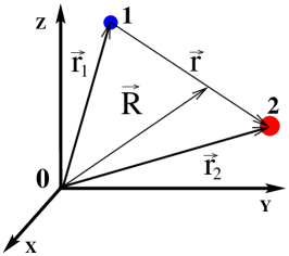
Figure 1: Two particles 1 and 2 in the absolute and c.m.-rel. Cartesian coordinate systems.

On the other hand, the formulation of the two-particle problem in the c.m. and rel. coordinates complicates the treatment of the trapping potential, because its original separability in the absolute Cartesian coordinates $\vec{r}_{j}$ is lost in the c.m.-rel. system. Only within the harmonic approximation for the trapping potential and for two identical atoms in the same internal state there is complete separability in c.m.-rel. coordinates Blume and Greene (2002). If the true atom-atom interaction is furthermore replaced by a $\delta$-function pseudopotential, the corresponding Schrödinger equation possesses an analytical solution for isotropic and some anisotropic harmonic traps Busch et al. (1998); Idziaszek and Calarco (2005). However, even within the harmonic approximation the separability is lost, if the two atoms experience different trapping potentials. This is the case, if a heteronuclear system or two identical atoms in different electronic states are considered. In the general case of a treatment beyond the harmonic approximation and, especially, if the atoms are spread over more than one potential well, there is evidently no separability at all.

In order to keep the flexibility with respect to the interparticle interaction and the advantage of its simple handling by using spherical c.m. and rel. coordinates, the optical-lattice potential has to be brought into a form that is convenient for its numerical treatment in those coordinates. This is done in two steps. First, a Taylor expansion of the sinusoidal trapping potential (3) is performed in Cartesian c.m. and rel. coordinates (Sec. II.2). The result is then transformed into spherical coordinates using an expansion in spherical harmonics (Sec. II.3).

II.2 Taylor expansion of the optical-lattice potential

The optical-lattice potential for both particles in Eq. (3) is given in the Cartesian c.m.-rel. coordinates $\vec{R}_{c}$ and $\vec{r}_{c}$ ($c=x,y,z$) as

$$\displaystyle\hat{\rm{V}}(\vec{R},\vec{r}\,) =\sum\limits_{i=1}^{2}\sum\limits_{c=x,y,z}V_{c}^{i}$$

$$\hskip 28.45274pt\times\sin^{2}(k_{c}[R_{c}+(-1)^{i-1}\mu_{\eta_{i}}r_{c}])$$ (5)

where the index $\displaystyle\eta_{i}=i+(-1)^{i-1}$ was introduced for compactness. Using the standard trigonometric relations the optical-lattice potential can be rewritten in the more suitable form

$$\hat{\rm V}(\vec{R},\vec{r}\,)=\frac{1}{2}\sum\limits_{i=1}^{2}\sum\limits_{c=x,y,z}V^{i}_{c}\left[1+(-1)^{\eta_{i}}\sin(2k_{c}R_{c})\right.{}\\ {}\left.\times\,\sin(2k_{c}r_{c}\mu_{\eta_{i}})-\cos(2k_{c}R_{c})\cos(2k_{c}r_{c}\mu_{\eta_{i}})\right]\,.$$ (6)

In order to achieve a maximal separation of the coordinates $\vec{R}$ and $\vec{r}$ the trigonometric functions in Eq. (6) are expanded in Taylor series around the origin of the c.m. and rel. coordinates,

$$\displaystyle\sin(2k_{c}R_{c})\sin(2k_{c}r_{c}\mu_{\eta_{s}})=\sum\limits_{j=0}^{\infty}\sum\limits_{i=0}^{\infty}\frac{(-1)^{i+j}}{(2i+1)!(2j+1)!}$$

$$\times\,(2k_{c})^{2i+1}(2k_{c}\mu_{\eta_{s}})^{2j+1}R_{c}^{2i+1}r_{c}^{2j+1}\,,$$ (7)

$$\cos(2k_{c}R_{c})\cos(2k_{c}r_{c}\mu_{\eta_{s}})=\sum\limits_{t=0}^{\infty}\sum\limits_{k=0}^{\infty}\frac{(-1)^{k+t}}{(2k)!(2t)!}$$

$$\times\,(2k_{c})^{2k}(2k_{c}\mu_{\eta_{s}})^{2t}R_{c}^{2k}r_{c}^{2t}\,.$$ (8)

In a practical numerical implementation, the infinite sum must be truncated. If, for example, the expansion is restricted up to the $\displaystyle(2n)$th degree (with the order $n=1,2,3,...$), the infinite summations in Eqs. (7) and (8) are changed, since the indices fulfill

$$2i+1+2j+1\leq 2n\quad\text{with}$$

$$i\leq n-1-j\quad\text{and}\quad j\leq n-1\,,\vskip 3.0pt plus 1.0pt minus 1.0pt$$

$$2k+2t\leq 2n\quad\text{with}$$

$$k\leq n-t\quad\text{and}\quad t\leq n\,.$$ (9)

Hence, the optical-lattice potential can be approximated by a Taylor expansion of degree $\displaystyle(2n)$ as

$$\hat{\rm V}(\vec{R},\vec{r})\approx\frac{1}{2}\sum\limits_{s=1}^{2}\sum\limits_{c=x,y,z}V^{s}_{c}\Biggl{[}1+(-1)^{\eta_{s}}\sum\limits_{j=0}^{n-1}{}\\ {}\times\,\sum\limits_{i=0}^{n-1-j}\mathbb{C}_{ijcs}^{\text{sin}}R_{c}^{2i+1}r_{c}^{2j+1}-\,\sum\limits_{t=0}^{n}\sum\limits_{k=0}^{n-t}\mathbb{C}_{tkcs}^{\text{cos}}R_{c}^{2k}r_{c}^{2t}\Biggr{]}$$ (10)

where the coefficients

$$\mathbb{C}_{tkcs}^{\text{cos}}=\frac{(-1)^{k+t}}{(2k)!(2t)!}(2k_{c})^{2(k+t)}\mu_{\eta_{s}}^{2t}\,,$$ (11)

$$\mathbb{C}_{ijcs}^{\text{sin}}=\frac{(-1)^{i+j}}{(2i+1)!(2j+1)!}(2k_{c})^{2(i+j+1)}\mu_{\eta_{s}}^{2j+1}$$ (12)

are introduced for compactness.

Using Eq. (10) it is possible to split the optical-lattice potential according to

$$\hat{\rm V}(\vec{R},\vec{r})=\hat{\rm v}_{\rm c.m.}(\vec{R})+\hat{\rm v}_{\rm rel.}(\vec{r})+\hat{\rm W}(\vec{R},\vec{r})$$ (13)

into $\hat{\rm v}_{\rm c.m.}$ and $\hat{\rm v}_{\rm rel.}$ that contain all terms depending solely on the c.m. coordinate and the rel. coordinate, respectively. The coupling terms between c.m. and rel. motion are now contained in $\hat{\rm W}$. The three components of $\hat{\rm{V}}$ are

$$\hat{\rm v}_{\rm c.m.}(\vec{R})=-\frac{1}{2}\sum\limits_{s=1}^{2}\sum\limits_{c=x,y,z}V^{s}_{c}\sum\limits_{k=1}^{n}\mathbb{C}_{0kcs}^{\text{cos}}R_{c}^{2k}$$ (14)

$$\hat{\rm v}_{\rm rel.}(\vec{r})=-\frac{1}{2}\sum\limits_{s=1}^{2}\sum\limits_{c=x,y,z}V^{s}_{c}\sum\limits_{t=1}^{n}\mathbb{C}_{t0cs}^{\text{cos}}r_{c}^{2t}$$ (15)

$$\hat{\rm W}(\vec{R},\vec{r})=\frac{1}{2}\sum\limits_{s=1}^{2}\sum\limits_{c=x,y,z}V^{s}_{c}\Biggl{[}(-1)^{\eta_{s}}{}\\ {}\times\,\sum\limits_{j=0}^{n-1}\sum\limits_{i=0}^{n-1-j}\mathbb{C}_{ijcs}^{\text{sin}}R_{c}^{2i+1}r_{c}^{2j+1}-\sum\limits_{t=1}^{n}\sum\limits_{k=1}^{n-t}\mathbb{C}_{tkcs}^{\text{cos}}R_{c}^{2k}r_{c}^{2t}\Biggr{]}\,.$$ (16)

Note that the sum $\sum\limits_{k=1}^{0}$ that occurs for $n=1$ in the second term of Eq. (16) does not indicate an inverse summation but its absence, i.e., no sum at all.

As a result of the Taylor expansion the Hamiltonian (1) is transformed into the more convenient form

$$\hat{\rm H}(\vec{R},\vec{r}\,)=\hat{\rm h}_{\rm c.m.}(\vec{R}\,)+\hat{\rm h}_{\rm rel.}(\vec{r}\,)+\hat{\rm W}(\vec{R},\vec{r}\,)$$ (17)

with

$$\displaystyle\hat{\rm h}_{\rm c.m.}(\vec{R}\,)=\hat{\rm t}_{\rm c.m.}(\vec{R}\,)+\hat{\rm v}_{\rm c.m.}(\vec{R}\,),$$ (18)

$$\displaystyle\hat{\rm h}_{\rm rel.}(\vec{r}\,)=\hat{\rm t}_{\rm rel.}(\vec{r}\,)+\hat{\rm v}_{\rm rel.}(\vec{r}\,)+\hat{\rm u}(r)$$ (19)

where we introduced $\hat{\rm t}_{\rm rel.}$ and $\hat{\rm t}_{\rm c.m.}$ for the kinetic-energy operators of the c.m. and the rel. motion, respectively. It is worth emphasizing that in the present formulation only the truly non-separable terms (represented by products of the c.m. and rel. coordinates) are left in the coupling term $\hat{\rm W}$. All separable terms of the optical lattice potential are included into the c.m. and rel. Hamiltonians $\hat{\rm h}_{\rm c.m.}$ and $\hat{\rm h}_{\rm rel.}$, respectively.

In fact, there is a specific case in which the optical-lattice potential in Eq. (6) can be brought into the form of Eq. (13) and thus the Hamiltonian (17) can be obtained without performing the Taylor expansion. This is the case for two identical particles that are both in the same state, if they are deposited in a cubic lattice with equal intensities and $k$ vectors along each of the spatial directions Bolda et al. (2005). If all these conditions are satisfied, then Eq. (6) can be written as

$$\displaystyle\hat{\rm v}_{\rm c.m.}(\vec{R})=2V_{0}\sum\limits_{c=x,y,z}\sin^{2}\left(kR_{c}\right)\,,$$ (20)

$$\displaystyle\hat{\rm v}_{\rm rel.}(\vec{r})=2V_{0}\sum\limits_{c=x,y,z}\sin^{2}\left(\frac{kr_{c}}{2}\right)\,,$$ (21)

$$\displaystyle\hat{\rm W}(\vec{R},\vec{r})=-4V_{0}\sum\limits_{c=x,y,z}\sin^{2}(kR_{c})\sin^{2}\left(\frac{kr_{c}}{2}\right)\,.$$ (22)

Noteworthy, the sum of the $\sin^{2}$-shaped lattice potentials for the two individual particles transforms into $\sin^{2}$-shaped potentials for both the c.m. and rel. motion, though the one of the c.m. motion possesses a different periodicity. In fact, this is also true in the here considered general case of a heteronuclear atom pair in an orthorhombic lattice. This is easily seen by extending the Taylor expansions in Eqs. (14) to (16) which gives

$$\lim_{n\rightarrow\infty}\hat{\rm v}_{\rm c.m.}(\vec{R})=\sum\limits_{s=1}^{2}\sum\limits_{c=x,y,z}V^{s}_{c}\sin^{2}(k_{c}R_{c})\,,$$ (23)

$$\lim_{n\rightarrow\infty}\hat{\rm v}_{\rm rel.}(\vec{r})=\sum\limits_{s=1}^{2}\sum\limits_{c=x,y,z}V^{s}_{c}\sin^{2}(k_{c}r_{c}\mu_{\eta_{s}})\,,$$ (24)

$$\lim_{n\rightarrow\infty}\hat{\rm W}(\vec{R},\vec{r})=\frac{1}{2}\sum\limits_{s=1}^{2}\sum\limits_{c=x,y,z}V^{s}_{c}\Biggl{[}(-1)^{\eta_{s}}{}\\ {}\sin(2k_{c}R_{c})\sin(2k_{c}r_{c}\mu_{\eta_{s}}){}\\ {}-\,\sum\limits_{t=1}^{n}\sum\limits_{k=1}^{n-t}\mathbb{C}_{tkcs}^{\text{cos}}R_{c}^{2k}r_{c}^{2t}\Biggr{]}\,.$$ (25)

Since an analytical solution for the $\sin^{2}$-like lattice and non-interacting particles exists Kohn (1959), those uncoupled known solutions of the Schrödinger equations with the Hamiltonians in Eqs. (23) and (24) could be used as a basis for solving the coupled problem. However, due to the presence of the central interaction potential a transformation to the spherical coordinate system is advantageous, since $\hat{\rm\mathcal{U}}(\vec{r})=\hat{\rm\mathcal{U}}(\sqrt{x^{2}+y^{2}+z^{2}})$ does normally not allow for a simple solution in Cartesian coordinates. However, this change of coordinates is inconvenient, since the mentioned analytical solutions of the $\sin^{2}$ potential do not split into simple products of the radial and angular parts. Since $\hat{\rm\mathcal{U}}$ can in principle have any possible functional form, it is more convenient to transform the optical-lattice potential into a form that is suitable for a calculation in spherical coordinates. This is done in the following subsection by an expansion in spherical harmonics.

II.3 Expansion of the optical-lattice potential in spherical harmonics

II.3.1 Auxiliary functions $\mathbb{Y}_{lmt}^{c}$ and $\tilde{\mathbb{Y}}_{lmt}^{c}$

In order to express the optical-lattices potentials $\hat{\rm v}_{\rm c.m.}$, $\hat{\rm v}_{\rm rel.}$, and $\hat{\rm W}$ in Eqs. (14), (15), and (16), respectively, in terms of the spherical harmonics $Y_{l}^{m}$, the corresponding polynomials in the Cartesian coordinates $\vec{r}_{c}^{\,t}$ and $\vec{R}_{c}^{t}$ have to be rewritten as radial part times an angular function, i. e., as $r_{c}^{t}\,F_{t}^{c}(\theta,\phi)$ and $R_{c}^{t}\,F_{t}^{c}(\theta,\phi)$, respectively. Every function of the angles $\phi$ and $\theta$ and thus $F_{t}^{c}$ can be expanded in spherical harmonics according to

$$F_{t}^{c}(\theta,\phi)=\sum\limits_{l=0}^{\infty}\sum\limits_{m=-l}^{l}\mathbb{Y}_{lmt}^{c}Y_{l}^{m}(\theta,\phi)$$ (26)

where the projection coefficients $\mathbb{Y}^{c}_{lmt}$ are given as

$$\displaystyle\mathbb{Y}_{lmt}^{c}=(-1)^{m}A_{l-m}\int_{\Omega}d\Omega\,F_{t}^{c}(\theta,\phi){P_{l}^{-m}}(\theta)e^{-{\rm i}m\phi}\,.$$ (27)

In Eq. (27) ${\rm i}$ stands for the imaginary unit, $\displaystyle P_{l}^{m}(\theta)$ are the associated Legendre polynomials and $\displaystyle A_{l-m}$ is a constant prefactor which is defined by

$$A_{lm}=\sqrt{\frac{2l+1}{4\pi}\frac{(l-m)!}{(l+m)!}}\,.$$ (28)

Finally, the integral over the angular arguments is $\int_{\Omega}d\Omega=\int\limits_{0}^{\pi}d\theta\int\limits_{0}^{2\pi}d\phi\sin(\theta)$. Due to their different properties, it is useful to distinguish two types of the expansion coefficients $\mathbb{Y}_{lmt}^{c}$, those with even values of $t$ and those with odd $t$. The latter ones are in the following denoted as $\tilde{\mathbb{Y}}_{lmt}^{c}$. According to Eqs. (14) and (15) only even powers of the Cartesian c.m. and rel. coordinates occur in the Taylor expansions of $\hat{\rm v}_{\rm c.m.}$ and $\hat{\rm v}_{\rm rel.}$ and thus only $\mathbb{Y}_{lmt}^{c}$ has to be evaluated in those cases. However, the coupling term $\hat{\rm W}$ contains additionally odd powers of $R_{c}$ and $r_{c}$ and thus requires also the calculation of $\tilde{\mathbb{Y}}_{lmt}^{c}$.

First, the calculation of the even-order coefficients $\mathbb{Y}_{lmt}^{x}$, $\mathbb{Y}_{lmt}^{y}$, and $\mathbb{Y}_{lmt}^{z}$ will be considered. They contain the functions $F_{t}^{c}(\theta,\,\phi)$ that are equal to $\cos^{2t}(\phi)\sin^{2t}(\theta)$ ($c=x$), $\sin^{2t}(\phi)\sin^{2t}(\theta)$ ($c=y$), and $\cos^{2t}(\theta)$ ($c=z$). Consider the integral for $\displaystyle\mathbb{Y}_{lmt}^{x}$. The derivation of $\displaystyle\mathbb{Y}_{lmt}^{x}$ is simplified by applying the Euler formula for $\displaystyle\cos^{2t}(\phi)$ and making use of Eq. (1.111) in Ref. Gradshteyn and Ryzhik (2007). The introduction of the new integration variable $\xi=\cos{(\theta)}$ transforms the integration limits in (27) from $[0,\pi]$ of $\theta$ to $[-1,1]$ for $\xi$. Clearly, the integral is non-zero only, if the integrand is symmetric in the $[-1,1]$ interval. At this point it is important to note that the associated Legendre function $\displaystyle P_{l}^{m}$ is even, if the $l+|m|$ sum is even, and odd otherwise. Since the summation index $k$ in Eq. (1.111) from Ref. Gradshteyn and Ryzhik (2007) is an integer that lies in the interval $\displaystyle 0\leq k\leq 2t$, the relation $\displaystyle-2t\leq m\leq 2t$ is valid. Hence, the $m$ index is always even. Therefore, the integral is non-zero only for even values of $l$. Additionally, there are, of course, the natural restrictions on the $l$ and $m$ coefficients, i. e., $\displaystyle l\geq 0$ and $\displaystyle|m|\leq l$. Another important fact is that the functions $\displaystyle P_{l>2t}^{|m|\leq l,|m|\leq 2t}(\xi)$ are oscillatory in the interval $[-1,1]$ and the symmetry of the integrand causes the contribution of negative and positive parts to cancel out, leading to a vanishing integral. Hence, one more restriction on $l$ is $\displaystyle l\leq 2t$. Additionally, Eq. (7.132.1) for the integral over the associated Legendre function together with Eqs. (8.339.2), (8.339.3) and (8.331.1) (all from Ref. Gradshteyn and Ryzhik (2007)) were used in the calculations.

Summarizing all the steps mentioned above and collecting the indices that do not give trivial zero contributions, the analytical form of $\displaystyle\mathbb{Y}_{lmt}^{x}$ can be given as

$$\mathbb{Y}_{lmt}^{x}=(-1)^{\frac{l+m}{2}}2^{-\frac{m}{2}-t+2}A_{l-m}\,\pi\,{2t\choose t+\frac{m}{2}}\\ \displaystyle\times\,\frac{(t-\frac{m}{2})!(t+\frac{m}{2})!(l-m-1)!!}{(t-\frac{l}{2})!(\frac{l}{2}+\frac{m}{2})!(2t+l+1)!!}\,,\\ l,m\text{ even,}\;-2t\leq m\leq 2t,\,\,|m|\leq l,\,\,l\leq 2t\,.$$ (29)

The derivation of the $\mathbb{Y}_{lmt}^{y}$ coefficient is similar to the one for $\mathbb{Y}_{lmt}^{x}$ and results in

$$\mathbb{Y}_{lmt}^{y}=(-1)^{\frac{m}{2}}\mathbb{Y}_{lmt}^{x}$$ (30)

with the same constraints for the indices as for $\mathbb{Y}_{lmt}^{x}$. In order to derive the $\displaystyle\mathbb{Y}_{lmt}^{z}$ coefficients, Eqs. (7.231.1) and (8.752.2) from Ref. Gradshteyn and Ryzhik (2007) were additionally used. This gives

$$\displaystyle\mathbb{Y}_{lmt}^{z}=A_{l0}\,(-1)^{\frac{l}{2}}\pi\delta_{m,0}\frac{2^{\frac{l}{2}+2}(2t-1)!!}{(l+2t+1)!!}\prod\limits_{i=0}^{l/2-1}(-t+i)\,,$$

$$l\text{ even,}\,\,l\leq 2t\,,$$ (31)

where $\delta_{i,j}$ is Kronecker’s delta.

Finally, the odd-order coefficients $\tilde{\mathbb{Y}}_{lmj}^{x}$, $\tilde{\mathbb{Y}}_{lmj}^{y}$, and $\tilde{\mathbb{Y}}_{lmj}^{z}$ have to be calculated efficiently. They contain the $F_{t}^{c}(\theta\,,\phi)$ functions that are equal to $\cos^{2j+1}(\phi)\sin^{2j+1}(\theta)$, $\sin^{2j+1}(\phi)\sin^{2j+1}(\theta)$, and $\cos^{2j+1}(\theta)$, respectively. The $\displaystyle\tilde{\mathbb{Y}}_{lmt}^{c}$ coefficients can also be calculated analytically. Consider, for example, the integral for $\tilde{\mathbb{Y}}_{lmj}^{x}$. Application of the Euler formula for the $\displaystyle\cos^{2j+1}(\phi)$ term and use of Eqs. (1.111) and (7.231.2) from Ref. Gradshteyn and Ryzhik (2007) leads to

$$\tilde{\mathbb{Y}}_{lmj}^{x}=(-1)^{\frac{l+m}{2}}\displaystyle 2^{\frac{3-2j-m}{2}}A_{l-m}{2j+1\choose j+\displaystyle\frac{m+1}{2}}{}\\ {}\times\,\pi\,\frac{\left(\frac{2j+1-m}{2}\right)!\left(\frac{2j+1+m}{2}\right)!(l-m-1)!!}{\left(\frac{2j+1-l}{2}\right)!\left(\frac{m+l}{2}\right)!(2j+l+2)!!}\,,{}\\ {}l,m\text{ are odd,}\,\,-2j-1\leq m\leq 2j+1,\,\,l\leq 2j+1\,.$$ (32)

The derivation of $\tilde{\mathbb{Y}}_{lmj}^{y}$ is also similar to the one of $\tilde{\mathbb{Y}}_{lmj}^{x}$ and results in

$$\displaystyle\tilde{\mathbb{Y}}_{lmj}^{y}={\rm i}\,\displaystyle(-1)^{\frac{m-3}{2}}\tilde{\mathbb{Y}}_{lmj}^{x}\,$$ (33)

with the same constraints on the indices as for $\tilde{\mathbb{Y}}_{lmj}^{x}$. Finally, $\tilde{\mathbb{Y}}_{lmj}^{z}$ is given by

$$\tilde{\mathbb{Y}}_{lmj}^{z}=A_{l0}4\pi\delta_{m,0}(-2)^{\frac{l-1}{2}}\frac{(2j+1)!!}{(2j+l+2)!!}\prod\limits_{i=0}^{\frac{l-3}{2}}(-j+i)$$ (34)

II.3.2 Final form of the Hamiltonian

The final expression for the optical-lattice potential is obtained by inserting $F_{t}^{c}(\theta,\phi)$ as defined in Eq. (26) for the angular part of the polynomials of $\vec{R}$ and $\vec{r}$ occurring in Eqs. (14), (15), and (16). For the three terms

$$\hat{\rm v}_{\rm c.m.}(R,\Theta,\Phi)=-\frac{1}{2}\sum\limits_{s=1}^{2}\sum\limits_{c=x,y,z}V^{s}_{c}\sum\limits_{k=1}^{n}\mathbb{C}_{0kcs}^{\text{cos}}\,R^{2k}{}\\ {}\times\,\sum\limits_{L=0,\{2\}}^{2k}\sum\limits_{M=-L,\{2\}}^{L}\mathbb{Y}_{LMk}^{c}Y_{L}^{M}(\Theta,\Phi)\,,$$ (35)

$$\hat{\rm v}_{\rm rel.}(r,\theta,\phi)=-\frac{1}{2}\sum\limits_{s=1}^{2}\sum\limits_{c=x,y,z}V^{s}_{c}\sum\limits_{t=1}^{n}\mathbb{C}_{t0cs}^{\text{cos}}\,r^{2t}{}\\ {}\times\,\sum\limits_{l=0,\{2\}}^{2t}\sum\limits_{m=-l,\{2\}}^{l}\mathbb{Y}_{lmt}^{c}Y_{l}^{m}(\theta,\phi)\,,$$ (36)

and

$$\hat{\rm W}(R,\Theta,\Phi,r,\theta,\phi)=\frac{1}{2}\sum\limits_{s=1}^{2}\sum\limits_{c=x,y,z}V^{s}_{c}{}\\ {}\times\,\left((-1)^{\eta_{s}}\sum\limits_{j=0}^{n-1}\sum\limits_{i=0}^{n-1-j}\mathbb{C}_{ijcs}^{\text{sin}}R^{2i+1}r^{2j+1}\right.{}\\ {}\times\,\sum\limits_{l=1,\{2\}}^{2j+1}\left[\tilde{\mathbb{Y}}_{l0j}^{c}Y_{l}^{0}(\theta,\phi)+\sum\limits_{m=-l,\{2\}}^{l}\tilde{\mathbb{Y}}_{lmj}^{c}Y_{l}^{m}(\theta,\phi)\right]{}\\ {}\times\,\sum\limits_{L=1,\{2\}}^{2i+1}\left[\tilde{\mathbb{Y}}_{L0i}^{c}Y_{L}^{0}(\Theta,\Phi)+\sum\limits_{M=-L,\{2\}}^{L}\tilde{\mathbb{Y}}_{LMi}^{c}Y_{L}^{M}(\Theta,\Phi)\right]{}\\ {}-\,\sum\limits_{t=1}^{n}\sum\limits_{k=1}^{n-t}\mathbb{C}_{tkcs}^{\text{cos}}R^{2k}r^{2t}\sum\limits_{l=0,\{2\}}^{2t}\sum\limits_{m=-l,\{2\}}^{l}\mathbb{Y}_{lmt}^{c}Y_{l}^{m}(\theta,\phi){}\\ {}\times\,\left.\sum\limits_{L=0,\{2\}}^{2k}\sum\limits_{M=-L,\{2\}}^{L}\mathbb{Y}_{LMk}^{c}Y_{L}^{M}(\Theta,\Phi)\right)$$ (37)

is found where, e. g., $\sum\limits_{l=0,\{2\}}^{2t}$ stands for $\sum\limits_{l=0,2,4,\dots}^{2t}$. In Eq. (37) $\tilde{\mathbb{Y}}_{l0j}^{x}=\tilde{\mathbb{Y}}_{l0j}^{y}=0$ and $\tilde{\mathbb{Y}}_{lmj}^{z}=0$ for $m\neq 0$ is implied.

As a result of adopting spherical c.m. and rel. coordinates the Hamiltonian

$$\displaystyle\hat{\rm H}(r,\theta,\phi,R,\Theta,\Phi) =\hat{\rm h}_{\rm rel.}(r,\theta,\phi)+\hat{\rm h}_{\rm c.m.}(R,\Theta,\Phi)$$

$$\quad+\hat{\rm W}(r,\theta,\phi,R,\Theta,\Phi)$$ (38)

is obtained with

$$\displaystyle\hat{\rm h}_{\rm c.m.}(R,\Theta,\Phi)=-\frac{1}{2{\rm M}}\left[\frac{\partial^{2}}{\partial R^{2}}\right. \left.+\frac{2}{R}\frac{\partial}{\partial R}-\frac{{{\bf\hat{I}}^{2}_{\rm c.m.}}}{R^{2}}\right]$$

$$\hskip 5.69046pt+\hat{\rm v}_{\rm c.m.}(R,\Theta,\Phi)$$ (39)

and

$$\displaystyle\hat{\rm h}_{\rm rel.}(r,\theta,\phi)=-\frac{1}{2\mu}\left[\frac{\partial^{2}}{\partial r^{2}}\right. \left.+\frac{2}{r}\frac{\partial}{\partial r}-\frac{{{\bf\hat{I}}^{2}_{\rm rel.}}}{r^{2}}\right]+\hat{\rm u}(r)$$

$$\hskip 5.69046pt+\hat{\rm v}_{\rm rel.}(r,\theta,\phi)\,.$$ (40)

In these equations $\hat{\rm\bf I}_{\rm c.m.}$ and $\hat{\rm\bf I}_{\rm rel.}$ are the operators of angular momentum, $\mu=m_{1}m_{2}/(m_{1}+m_{2})$ is the reduced mass, and ${\rm M}=m_{1}+m_{2}$ is the total mass of the two particles.

The key achievement is that now all terms in the Hamiltonian are at most a sum over products of functions that depend only on a single coordinate, i. e., $f_{1}(R)f_{2}(\Theta)f_{3}(\Phi)g_{1}(r)g_{2}(\theta)g_{3}(\phi)$. As a result all required integrals are at most products of one-dimensional integrals.

II.3.3 Finite and $\cos^{2}$ lattices

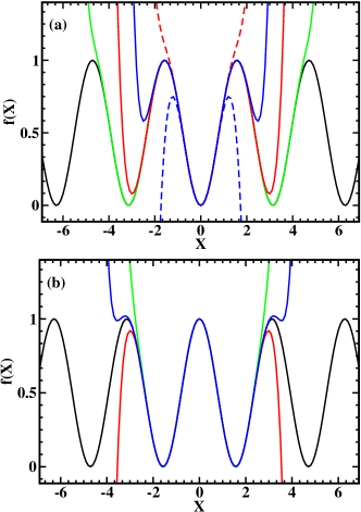
Figure 2: (a) The $\sin^{2}(x)$ function (black solid) together with the 2nd- (blue dashes), 3rd- (red dashes), 5th- (blue solid), 7th- (red solid) and 11th-order (green solid) expansion of the Taylor series. (b) The $\cos^{2}(x)$ function (black) together with the 6th- (green), 7th- (red) and 8th-order (blue) expansion of the Taylor series.

For practical reasons, the infinite Taylor expansion of the $\sin^{2}$ potential has to be truncated in a calculation. In such a situation convergence of the results with respect to the expansion length is usually aimed for. However, in the present case some caution has to be applied in such a study and the interpretation of its outcome Grishkevich and Saenz (2009). The problem is due to the fact that the Taylor expansion is performed around the origin. Hence the $\sin^{2}$ lattice is best described close to the origin, while the deviations increase with increasing distance from it. This is illustrated in Fig. 2(a) in which the $\sin^{2}$ lattice (along one coordinate) is compared to Taylor expansions of different order. While the 2nd-order expansion works already very well at and close to the origin, even the barrier height of the central well is not correctly described. On the other hand, the 3rd-order expansion that includes polynomials up to 6th order and may thus be called sextic potential agrees very well with the central well of the $\sin^{2}$ potential. The sextic potential is thus a very good choice for the investigation of the effects of anharmonicity on (tightly) bound states in a single site of an optical lattice Grishkevich and Saenz (2009). While increasing the order of the expansion by considering, e. g., the 5th- or 7th-order expansion improves the agreement with the $\sin^{2}$ potential further away from the origin, a problem occurs. The resulting potential possesses three wells, but the outer ones have a depth that differs from the correct one, as is also illustrated in Fig. 2(a). As a consequence, non-physical resonances may occur due to tunneling. Hence, a simple convergence study in which the Taylor expansion is expanded order by order is problematic. In fact, an even more severe problem is observed for all even-order expansions like the already discussed 2nd-order one. Those expansions tend to $-\infty$ for $x$ going to either $-\infty$ or $+\infty$ (or even in both cases as for the shown 2nd-order expansion). As a consequence, an infinite number of unphysical negative-energy states occur.

In conclusion, the present approach that is based on a Taylor expansion of the optical-lattice potential is especially suitable for describing finite optical lattices. With a judicious choice of the expansion of the $\sin^{2}$ potential the physics of single- triple-, or higher multiple-well potentials can be well described. For example, the $11$th-order expansion also shown in Fig. 2(a) provides a very good description of the physics in a triple-well potential Schneider et al. (2009). Clearly, even an expansion like the 5th-order one may be useful, if an asymmetric potential with different depths of the wells should be considered. Furthermore, with a sufficiently large number of wells even the physics of a complete optical lattice can be described in which the continuum states (or transitions to them) are involved. In that case convergence with respect to the number of wells (and not with respect to the expansion length) has to be achieved, since the true continuum is replaced by a correspondingly discretized spectrum. In fact, it may also be reminded that in most experiments involving ultracold atoms in optical lattices there is an additional confining potential and thus the whole (relevant) spectrum can be discrete.

An evident limitation of the $\sin^{2}$ lattice and its Taylor expansion discussed so far is that only finite lattices with an odd number of wells can easily be described. Clearly, in many situations also finite lattices with an even number of potential wells are of interest. The most prominent example is certainly the double-well potential that is also of special interest for quantum-information studies. The physics of few atoms in (one-dimensional) double-well potentials was recently studied, e. g., in Zöllner et al. (2008). The most straightforward extension of the present approach towards such potentials is by considering a Taylor expansion of the $\cos^{2}$ (or $\pi/2$-shifted $\sin^{2}$) potential

$$\hat{\rm{V}}^{\cos}(\vec{R},\vec{r})=\sum\limits_{s=1}^{2}\sum\limits_{c=x,y,z}V_{c}^{s}\sin^{2}(k_{c}c_{s}+\frac{\pi}{2})\,.$$ (41)

Using trigonometric relations the optical-lattice potential can be written in the more suitable form

$$\hat{\rm V}^{\cos}(\vec{R},\vec{r})=\frac{1}{2}\sum\limits_{s=1}^{2}\sum\limits_{c=x,y,z}V^{s}_{c}[1+(-1)^{s}\sin(2k_{c}R_{c}){}\\ {}\times\,\sin(2k_{c}r_{c}\mu_{\eta_{s}})+\,\cos(2k_{c}R_{c})\cos(2k_{c}r_{c}\mu_{\eta_{s}})]\,.$$ (42)

After derivations similar to the case of the $\sin^{2}$ potential the splitting of the optical lattice into the c.m. and rel. motion in the Cartesian frame yields

$$\displaystyle\hat{\rm v}_{0}^{\cos} =\sum\limits_{s=1}^{2}\sum\limits_{c=x,y,z}V^{s}_{c}$$ (43)

$$\hat{\rm v}_{\rm c.m.}^{\cos}(\vec{R}) =\frac{1}{2}\sum\limits_{s=1}^{2}\sum\limits_{c=x,y,z}V^{s}_{c}\sum\limits_{k=1}^{n}\mathbb{C}_{0kcs}^{\text{cos}}R_{c}^{2k}$$ (44)

$$\hat{\rm v}_{\rm rel.}^{\cos}(\vec{r}) =\frac{1}{2}\sum\limits_{s=1}^{2}\sum\limits_{c=x,y,z}V^{s}_{c}\sum\limits_{t=1}^{n}\mathbb{C}_{t0cs}^{\text{cos}}r_{c}^{2t}$$ (45)

$$\hat{\rm W}^{\cos}(\vec{R},\vec{r}) =\frac{1}{2}\sum\limits_{s=1}^{2}\sum\limits_{c=x,y,z}V^{s}_{c}\Biggl{[}(-1)^{s}\sum\limits_{j=0}^{n-1}$$ (46)

$$\times\,\sum\limits_{i=0}^{n-1-j}\mathbb{C}_{ijcs}^{\text{sin}}R_{c}^{2i+1}r_{c}^{2j+1}+\sum\limits_{t=1}^{n}\sum\limits_{k=1}^{n-t}\mathbb{C}_{tkcs}^{\text{cos}}R_{c}^{2k}r_{c}^{2t}\Biggr{]}$$

where the constant term $\hat{\rm v}_{0}^{\cos}$ appears that was zero for the $\sin^{2}$ case. Equations (43)-(46) are almost analogous to Eqs. (14)-(16) for the $\sin^{2}$-like potential. In Fig. 2(b) the $\cos^{2}$ lattice (along one coordinate) is shown together with Taylor expansions of different order. In this case, an even-order expansion should be used to avoid unphysical negative energy states. For example, while the 6th-order expansion provides a rather good representation of two neighbor wells in an optical lattice, the 7th-order expansion leads to negative energy states and does in fact even not represent the outer potential barriers properly. The 8th-order expansion is again rather good, but leads already to small artificial side minima.

Since the adopted expansions are independent for the three orthogonal directions $x$, $y$, and $z$, the present approach is capable of describing two particles in any combination of different lattices along those three directions. While, e. g., in Schneider et al. (2009) a true triple well was described using the 11th-order expansion of $\sin^{2}$ in one and a harmonic (1st-order) expansion in the two other directions, alternatively an array of $3\times 3\times 3$ lattice sites could be described equally well.

III Exact diagonalization

III.1 Schrödinger equations

After having formulated the optical lattice potential in a suitable form, the solution of the eigenvalue problem is described in the following. The Schrödinger equation with the Hamiltonian of (38)

$$\hat{\rm H}\,|\Psi_{i}\rangle=\mathcal{E}_{i}\,|\Psi_{i}\rangle\,,$$ (47)

is solved by expanding $\Psi$ in terms of configurations,

$$\Psi_{i}(\vec{R},\vec{r}\,)=\sum_{\kappa}\,C_{i,\kappa}\,\Phi_{\kappa}(\vec{R},\vec{r}\,)\,.$$ (48)

The configurations

$$\Phi_{\kappa}(\vec{R},\vec{r})=\varphi_{i_{\kappa}}(\vec{r}\,)\,\psi_{j_{\kappa}}(\vec{R}\,)$$ (49)

are products of the eigenfunctions of the Hamiltonians of rel. and c.m. motions, respectively, i. e., $\varphi$ and $\psi$ are solutions of

$$\hat{\rm h}_{\rm rel.}\,|\varphi_{i}\rangle=\epsilon_{i}^{\rm rel.}\,|\varphi_{i}\rangle\,$$ (50)

and

$$\hat{\rm h}_{\rm c.m.}\,|\psi_{j}\rangle=\epsilon_{j}^{\rm c.m.}\,|\psi_{j}\rangle.$$ (51)

Finally, the wavefunctions of rel. and c.m. motion that we denote as orbitals (in formal analogy to the one-particle solutions in electronic-structure calculations) are expressed in basis functions $\tilde{\varphi}$ and $\tilde{\psi}$ that are products of $B$ splines and spherical harmonics $Y_{l}^{m}$ for describing the radial and the angular parts, respectively,

$$\varphi_{i}(\vec{r}) =\sum\limits_{\mathbf{a}}\tilde{c}^{\rm rel.}_{i,\mathbf{a}}\,\tilde{\varphi}_{\mathbf{a}}$$ (52)

$$=\sum\limits_{\alpha=1}^{N_{r}}\sum\limits_{l=0}^{N_{l}}\sum\limits_{m=-l}^{l}\tilde{c}^{\rm rel.}_{i,\alpha lm}\,r^{-1}\,B_{\alpha}(r)Y_{l}^{m}(\theta,\phi)$$ (53)

and

$$\psi_{j}(\vec{R}) =\sum\limits_{\mathbf{b}}\tilde{c}^{\rm c.m.}_{j,\mathbf{b}}\,\tilde{\psi}_{\mathbf{b}}$$ (54)

$$=\sum\limits_{\beta=1}^{N_{R}}\sum\limits_{L=0}^{N_{L}}\sum\limits_{M=-L}^{L}\tilde{c}^{\rm c.m.}_{j,\beta LM}\,R^{-1}\,B_{\beta}(R)Y_{L}^{M}(\Theta,\Phi)\,.$$ (55)

In Eqs. (52) and (54), we introduced the compact indices $\mathbf{a}\equiv\alpha,l,m$ and $\mathbf{b}\equiv\beta,L,M$.

A specific basis set is characterized by the upper limits of angular momentum $N_{l}$ and $N_{L}$ in the spherical-harmonic expansions and the numbers $N_{r}$ and $N_{R}$ of $B$ splines used in the expansions in Eqs. (53) and (55) as well as their order $k_{\rm rel.}$ (and $k_{\rm c.m.}$) and knot sequences de Boor (1978); Bachau et al. (2001). The knot sequences define the ranges of $r$ and $R$ in which the wave functions are calculated, the so-called box, though it is, in fact, often a sphere as in the present case. If the box is chosen sufficiently large for a given finite trapping potential, all wavefunctions will have decayed before reaching the box boundaries. Otherwise, an artificial discretization occurs, if a zero-boundary condition at the wall of the box is enforced by removing the last $B$ spline. In this case an investigation of the convergence of the results with respect to the box size has to be performed.

The insertion of the expansions for $\varphi$ in (53) and $\psi$ in (55) into the Schrödinger equations (50) and (51), respectively, followed by a multiplication with either $\tilde{\varphi}_{i}^{*}$ or $\tilde{\psi}_{j}^{*}$ (from left) and integration over $\vec{r}$ or $\vec{R}$ leads to generalized matrix eigenvalue problems of the type

$$\mathbf{h}\mathbf{\tilde{c}}_{i}=\epsilon_{i}\,\mathbf{s}\mathbf{\tilde{c}}_{i}\,.$$ (56)

Their solutions provide the energies $\epsilon_{i}^{\rm rel.}$ (and $\epsilon_{j}^{\rm c.m.}$) as well as the coefficients $\tilde{c}^{\rm rel.}_{i,\mathbf{a}}$ (and $\tilde{c}^{\rm c.m.}_{j,\mathbf{b}}$). The latter define the rel. and c.m. orbitals $\varphi$ and $\psi$ according to Eqs. (52) and (54), respectively. Generalized eigenvalue equations occur due to the non-orthogonality of the $B$ splines. Furthermore, the explicit consideration of the factors $r^{-1}$ and $R^{-1}$ transforms the radial part of the Schrödinger equations into effective one-dimensional ones by removing the $\partial/\partial R$ and $\partial/\partial r$ terms in Eqs. (39) and (40). As a consequence, the diagonalizations provide in fact the solutions $r\varphi$ and $R\psi$ from which $\varphi$ and $\psi$ can, of course, easily be obtained. Since $r\varphi$ and $R\psi$ vanish for $r\rightarrow 0$ and $R\rightarrow 0$, respectively, this additional boundary condition is implemented by removing the first $B$ spline. Together with the corresponding boundary condition at the outer box boundaries, the summations in Eqs. (53) and (55) change into $\sum_{\alpha=2}^{N_{r}-1}$ and $\sum_{\beta=2}^{N_{r}-1}$, respectively. In fact, the actual implementation of the code is flexible with respect to different choices of the boundary conditions at the origin of rel. and c.m. motions, but in the following only the standard use based on the reduced summation limits is considered explicitly for reasons of better readability.

Once the eigenvectors $\varphi$ and $\psi$ are obtained, a set of configurations $\Phi$ is built according to Eq. (49). Again, insertion of the expansion for $\Psi$ in Eq. (48) into the Schrödinger equation (47), multiplication with $\Phi_{k}^{*}$ (from left), and integration over $\vec{r}$ and $\vec{R}$ yields the matrix eigenvalue equation

$$\mathbf{H}\mathbf{C}_{i}=\mathcal{E}_{i}\,\mathbf{C}_{i}\,.$$ (57)

Due to the orthonormality of the orbitals $\varphi$ and $\psi$ also the configurations $\Phi$ are orthonormal. Therefore, the overlap matrix is equal to the identity and Eq. (57) is an ordinary eigenvalue problem.

III.2 Matrix elements

In order to set up the matrix eigenvalue problems in Eqs. (56) and (57), the corresponding matrices

$$h_{\mathbf{a},\mathbf{a}^{\prime}}^{\rm rel.}=\langle\tilde{\varphi}_{\mathbf{a}}|\hat{\rm h}_{\rm rel.}|\tilde{\varphi}_{\mathbf{a}^{\prime}}\rangle\,, s_{\mathbf{a},\mathbf{a}^{\prime}}^{\rm rel.}=\langle\tilde{\varphi}_{\mathbf{a}}|\tilde{\varphi}_{\mathbf{a}^{\prime}}\rangle\,,$$ (58)

$$h_{\mathbf{b},\mathbf{b}^{\prime}}^{\rm c.m.}=\langle\tilde{\psi}_{\mathbf{b}}|\hat{\rm h}_{\rm c.m.}|\tilde{\psi}_{\mathbf{b}^{\prime}}\rangle\,, s_{\mathbf{b},\mathbf{b}^{\prime}}^{\rm c.m.}=\langle\tilde{\psi}_{\mathbf{b}}|\tilde{\psi}_{\mathbf{b}^{\prime}}\rangle$$ (59)

and

$$H_{\kappa,\kappa^{\prime}}=\langle\Phi_{\kappa}|\hat{\rm H}|\Phi_{\kappa^{\prime}}\rangle$$ (60)

have to be set up. As already mentioned, the overlap matrix elements between configurations are trivial,

$$S_{\kappa,\kappa^{\prime}}=\langle\Phi_{\kappa}|\Phi_{\kappa^{\prime}}\rangle{}\\ {}=\langle\varphi_{i_{\kappa}}\psi_{j_{\kappa}}|\varphi_{i_{\kappa^{\prime}}}\psi_{j_{\kappa^{\prime}}}\rangle=\delta_{i_{\kappa{\vphantom{{}^{\prime}}}},i_{\kappa^{\prime}}}\,\delta_{j_{\kappa\vphantom{{}^{\prime}}},j_{\kappa^{\prime}}}=\delta_{\kappa,\kappa^{\prime}}\,.$$ (61)

For convenience, the integrals over $B$ splines and their derivatives are denoted as

$$\mathbb{B}_{\partial^{\mu}\alpha\,\partial^{\nu}\alpha^{\prime}}^{\lambda}=\int\limits_{0}^{\infty}\,dr\,r^{\lambda}\frac{\partial^{\mu}B_{\alpha}(r)}{\partial r^{\mu}}\frac{\partial^{\nu}B_{\alpha^{\prime}}(r)}{\partial r^{\nu}}\,.$$ (62)

Furthermore, the index $\lambda$ and the orders of the derivatives $\mu$ (or $\nu$) are omitted for $\mu=0$ ($\nu=0$). For example, one has $\mathbb{B}_{\alpha\alpha^{\prime}}\equiv\mathbb{B}_{\partial^{0}\alpha\partial^{0}\alpha^{\prime}}^{0}$. Additionally, it is reminded that the character $\alpha$ is reserved for rel. motion matrix elements and $\beta$ for c.m. elements. Hence, the corresponding notation for the c.m. integral over $B$ splines analogous to Eq. (62) is

$$\mathbb{B}_{\partial^{\mu}\beta\,\partial^{\nu}\beta^{\prime}}^{\lambda}=\int\limits_{0}^{\infty}\,dR\,R^{\lambda}\frac{\partial^{\mu}B_{\beta}(R)}{\partial R^{\mu}}\frac{\partial^{\nu}B_{\beta^{\prime}}(R)}{\partial R^{\nu}}\,.$$ (63)

Since $B$ splines are polynomials, the integrals $\mathbb{B}$ can be calculated exactly by means of Gauss-Legendre quadrature. Due to the compactness (finite local support) of the $B$ splines the integration limits are in fact finite. If the two involved $B$ splines do not possess a common interval where both of them are non-zero, the integral vanishes. Therefore, only a very limited number of integrals has to be calculated and the resulting overlap and Hamiltonian matrices are sparse. In the following, all integrals that occur in the calculation are discussed individually.

III.2.1 Overlap

The overlap matrices between the basis functions $\tilde{\varphi}$ and $\tilde{\psi}$ are not equal to the identity matrix, but

$$s_{\mathbf{a},\mathbf{a^{\prime}}}^{\rm rel.}=\mathbb{B}_{\alpha\alpha^{\prime}}\displaystyle\int_{\Omega}\,d\Omega\,{Y_{l}^{m}}^{*}(\theta,\phi)Y_{l^{\prime}}^{m^{\prime}}(\theta,\phi)=\mathbb{B}_{\alpha\alpha^{\prime}}\delta_{ll^{\prime}}\delta_{mm^{\prime}}$$ (64)

and, similarly,

$$s_{\mathbf{b},\mathbf{b^{\prime}}}^{\rm c.m.}=\mathbb{B}_{\beta\beta^{\prime}}\delta_{LL^{\prime}}\delta_{MM^{\prime}}\,.$$ (65)

III.2.2 Kinetic energy

Since the basis functions are a product of a radial $B$ spline and a spherical harmonic, the action of the kinetic-energy operator on them is straightforwardly calculated. Using $\displaystyle{{\bf\hat{I}}^{2}_{\rm rel.}}Y_{l}^{m}(\theta,\phi)=l(l+1)Y_{l}^{m}(\theta,\phi)$ and $\displaystyle{{\bf\hat{I}}^{2}_{\rm c.m.}}Y_{L}^{M}(\Theta,\Phi)=L(L+1)Y_{L}^{M}(\Theta,\Phi)$, one finds

$$t_{\mathbf{a},\mathbf{a^{\prime}}}^{\rm rel.}=-\frac{1}{2\mu}\mathbb{B}_{\partial^{2}\alpha\,\alpha^{\prime}}\,\delta_{ll^{\prime}}\delta_{mm^{\prime}}+\frac{1}{2\mu}l(l+1)\,\mathbb{B}^{-2}_{\alpha\alpha^{\prime}}\,\delta_{ll^{\prime}}\delta_{mm^{\prime}}{}\\ ={}\frac{1}{2\mu}\left(\mathbb{B}_{\partial^{1}\alpha\,\partial^{1}\alpha^{\prime}}+l(l+1)\,\mathbb{B}^{-2}_{\alpha\alpha^{\prime}}\right)\delta_{ll^{\prime}}\delta_{mm^{\prime}}$$ (66)

for the rel. motion and analogously

$$t_{\mathbf{b},\mathbf{b^{\prime}}}^{\rm c.m.}=\frac{1}{2{\rm M}}\left(\mathbb{B}_{\partial^{1}\beta\,\partial^{1}\beta^{\prime}}+L(L+1)\,\mathbb{B}^{-2}_{\beta\beta^{\prime}}\right)\,\delta_{LL^{\prime}}\delta_{MM^{\prime}}$$ (67)

for the c.m. motion. Note, the second equality in Eq. (66) as well as Eq. (67) have to be (slightly) modified, if non-zero boundary conditions are applied at the origin and the box boundary.

III.2.3 Interparticle interaction

The matrix elements of the interparticle interaction potential are

$$u_{\mathbf{a},\mathbf{a^{\prime}}}=\delta_{ll^{\prime}}\delta_{mm^{\prime}}\,\int\limits_{0}^{\infty}\,dr\,\,u(r)B_{\alpha}(r)\,B_{\alpha^{\prime}}(r)\,.$$ (68)

The compactness of the $B$ splines turns the semi-indefinite integral into a definite one that has to be calculated only within a small spatial interval in which $B_{\alpha}$ and $B_{\alpha^{\prime}}$ (and, of course, $u(r)$) are simultaneously non-zero. In contrast to the case of the $\mathbb{B}$ integrals Gauss quadrature is in this case only exact, if $u(r)$ can be expressed in terms of a finite polynomial expansion. In practice, the quadrature converges quite well even with a relative small number of terms. This is again partly due to the fact that it is sufficient, if a polynomial expansion works well piecewise, i. e., only within small spatial intervals.

III.2.4 Separable part of the trapping potential

Using the property $\displaystyle{Y_{l_{t}}^{m_{t}}}^{*}(\theta,\phi)=(-1)^{m_{t}}{Y_{l_{t}}^{-m_{t}}}(\theta,\phi)$ the product of two spherical harmonics can be expressed as a sum of products between a spherical harmonic and the 3j-Wigner symbols,

$$Y_{l}^{m}(\theta,\phi)\,Y_{l_{t}}^{m_{t}}(\theta,\phi)={}\\ {}\sum\limits_{l_{t},m_{t}}\mathbb{A}^{0}_{l_{t}\,l\,l_{t}}\begin{pmatrix}l_{t}&l&l_{t}\\ m_{t}&m&m_{t}\end{pmatrix}\begin{pmatrix}l_{t}&l&l_{t}\\ 0&0&0\end{pmatrix}{Y_{l_{t}}^{m_{t}}}^{*}(\theta,\phi)\,.$$ (69)

Here, the coefficient

$$\mathbb{A}^{a}_{b\,c\,d}=(-1)^{a}\sqrt{\frac{(2b+1)(2c+1)(2d+1)}{4\pi}}\,$$ (70)

was introduced for compactness. The Gaunt coefficient may be obtained as Rasch and Yu (2003); Pinchon and Hoggan (2007)

$$\int_{\Omega}\,d\Omega\,Y_{l}^{m}(\theta,\phi)Y_{l_{t}}^{m_{t}}(\theta,\phi){Y_{l^{\prime}}^{m^{\prime}}}^{*}(\theta,\phi){}\\ {}=\sum\limits_{l_{t},m_{t}}\mathbb{A}^{m_{t}}_{l_{t}\,l\,l_{t}}\begin{pmatrix}l_{t}&l&l_{t}\\ m_{t}&m&m_{t}\end{pmatrix}\begin{pmatrix}l_{t}&l&l_{t}\\ 0&0&0\end{pmatrix}{}\\ {}\times\,\underbrace{\displaystyle\int_{\Omega}\,d\Omega\,{Y_{l_{t}}^{-m_{t}}}(\theta,\phi){Y_{l^{\prime}}^{m^{\prime}}}^{*}(\theta,\phi)}_{\displaystyle\delta_{l_{t}l^{\prime}}\,\delta_{-m_{t}m^{\prime}}}{}\\ {}=\mathbb{A}^{m^{\prime}}_{l_{t}\,l\,l^{\prime}}\begin{pmatrix}l_{t}&l&l^{\prime}\\ m_{t}&m&-m^{\prime}\end{pmatrix}\begin{pmatrix}l_{t}&l&l^{\prime}\\ 0&0&0\end{pmatrix}\,.$$ (71)

Making use of Eq. (71), the angular parts for the matrix elements of the trapping potential can be calculated straightforwardly. For the separable (uncoupled) parts

$$v_{\mathbf{a},\mathbf{a^{\prime}}}^{\rm rel.}=-\frac{1}{2}\sum\limits_{s=1}^{2}\sum\limits_{c=x,y,z}V^{s}_{c}\sum\limits_{t=1}^{n}\mathbb{C}_{t0cs}^{\text{cos}}\,\mathbb{B}^{2t}_{\alpha\,\alpha^{\prime}}\sum\limits_{{l_{t}}=0,\{2\}}^{2t}{}\\ {}\times\,\sum\limits_{{m_{t}}=-{l_{t}},\{2\}}^{{l_{t}}}\mathbb{Y}_{l_{t}{m_{t}}t}^{c}\mathbb{A}^{m^{\prime}}_{l_{t}\,l\,l^{\prime}}{}\begin{pmatrix}l_{t}&l&l^{\prime}\\ m_{t}&m&-m^{\prime}\end{pmatrix}\begin{pmatrix}l_{t}&l&l^{\prime}\\ 0&0&0\end{pmatrix}$$ (72)

and

$$V_{\mathbf{b},\mathbf{b^{\prime}}}^{\rm c.m.}=-\frac{1}{2}\sum\limits_{s=1}^{2}\sum\limits_{c=x,y,z}V^{s}_{c}\sum\limits_{k=1}^{n}\mathbb{C}_{0kcs}^{\text{cos}}\,\mathbb{B}^{2k}_{\beta\,\beta^{\prime}}{}\\ {}\times\,\sum\limits_{{L_{k}}=0,\{2\}}^{2k}\sum\limits_{{M_{k}}=-{L_{k}},\{2\}}^{{L_{k}}}\mathbb{Y}_{L_{k}{M_{k}}k}^{c}\mathbb{A}^{M^{\prime}}_{L_{k}\,L\,L^{\prime}}{}\\ {}\times\,\begin{pmatrix}L_{k}&L&L^{\prime}\\ M_{k}&M&-M^{\prime}\end{pmatrix}\begin{pmatrix}L_{k}&L&L^{\prime}\\ 0&0&0\end{pmatrix}\,.$$ (73)

are found for the rel. and c.m. matrix elements, respectively. With the aid of Eqs. (64), (66), (68), and (72) the rel. overlap and Hamiltonian matrices in Eqs. (58) are obtained. Insertion into Eq. (56) and subsequent diagonalization yields the uncoupled eigenenergies and eigenfunctions of the rel. motion, as discussed above. Analogously, Eqs. (65), (67), and (73) provide the overlap and Hamiltonian matrices in Eqs. (59), thus the eigenenergies and eigenfunctions of the uncoupled c.m. motion can be found.

III.2.5 Matrix elements of the coupled Hamiltonian

Finally, for obtaining the coupled solutions the Hamiltonian matrix elements $H_{\kappa,\kappa^{\prime}}$ in Eq. (60) have to be calculated. Remind, the total Hamiltonian $\hat{\rm H}$ was written as a sum of the uncoupled Hamiltonians of rel. and c.m. motion, $\hat{\rm h}_{\rm rel.},\hat{\rm h}_{\rm c.m.}$, and the coupling term $\hat{\rm W}$ (38). Since the configurations are build with the eigenfunctions $\varphi$ and $\psi$ of the uncoupled Hamiltonians, only the simple diagonal contribution

$$\displaystyle\langle\Phi_{\kappa}|\hat{\rm h}_{\rm c.m.} +\hat{\rm h}_{\rm rel.}|\Phi_{\kappa^{\prime}}\rangle{}$$

$$=\langle\varphi_{i_{\kappa}}\psi_{j_{\kappa}}|\hat{\rm h}_{\rm c.m.}+\hat{\rm h}_{\rm rel.}|\varphi_{i_{\kappa^{\prime}}}\psi_{j_{\kappa^{\prime}}}\rangle{}$$

$$=(\epsilon_{i_{\kappa}}^{\rm rel.}+\epsilon_{j_{\kappa}}^{\rm c.m.})\,\delta_{i_{\kappa\vphantom{{}^{\prime}}},i_{\kappa^{\prime}}}\,\delta_{j_{\kappa\vphantom{{}^{\prime}}},j_{\kappa^{\prime}}}$$ (74)

is obtained from $\hat{\rm h}_{\rm rel.}$ and $\hat{\rm h}_{\rm c.m.}$.

The remaining task is thus the calculation of the matrix elements that couple rel. and c.m. motions, i. e., the ones of $\hat{\rm W}$. They are given as

$$W_{\kappa,\kappa^{\prime}}=\frac{1}{2}\sum\limits_{s=1}^{2}\sum\limits_{c=x,y,z}V^{s}_{c}\Biggl{\{}(-1)^{\eta_{s}}\sum\limits_{j=0}^{n-1}(-1)^{j}\frac{(2k_{c}\mu_{\eta_{s}})^{2j+1}}{(2j+1)!}\sum\limits_{\alpha=2}^{N_{r}-1}\sum\limits_{l=0}^{N_{l}}\sum\limits_{m=-l}^{l}\tilde{c}_{p_{\kappa},\mathbf{a}}^{\rm rel.}\sum\limits_{\alpha^{\prime}=2}^{N_{r}-1}\sum\limits_{l^{\prime}=0}^{N_{l}}\sum\limits_{m^{\prime}=-l}^{l}\tilde{c}_{p_{\kappa^{\prime}},\mathbf{a}^{\prime}}^{\rm rel.}\,\mathbb{B}^{2j+1}_{\alpha\,\alpha^{\prime}}\\ \displaystyle\times\,\sum\limits_{l_{j}=1,\{2\}}^{2j+1}\Biggl{[}\Biggl{(}\tilde{\mathbb{Y}}_{l_{j}0j}^{c}\begin{pmatrix}l_{j}&l&l^{\prime}\\ 0&m&m^{\prime}\end{pmatrix}+\,\sum\limits_{m_{j}=-l_{j},\{2\}}^{l_{j}}\tilde{\mathbb{Y}}_{l_{j}m_{j}j}^{c}\begin{pmatrix}l_{j}&l&l^{\prime}\\ m_{j}&m&-m^{\prime}\end{pmatrix}\Biggr{)}\mathbb{A}^{m^{\prime}}_{l_{j}ll^{\prime}}\begin{pmatrix}l_{j}&l&l^{\prime}\\ 0&0&0\end{pmatrix}\Biggr{]}{}\\ {}\displaystyle\times\,\sum\limits_{i=0}^{n-1-j}(-1)^{i}\frac{(2k_{c})^{2i+1}}{(2i+1)!}\sum\limits_{\beta=2}^{N_{R}-1}\sum\limits_{L=0}^{N_{L}}\sum\limits_{M=-L}^{L}\tilde{c}_{q_{\kappa},\mathbf{b}}^{\rm c.m.}\sum\limits_{\beta^{\prime}=2}^{N_{R}-1}\sum\limits_{L^{\prime}=0}^{N_{L}}\sum\limits_{M^{\prime}=-L^{\prime}}^{L^{\prime}}\tilde{c}_{q_{\kappa^{\prime}},\mathbf{b}^{\prime}}^{\rm c.m.}\,\mathbb{B}^{2i+1}_{\beta\,\beta^{\prime}}{}\\ {}\displaystyle\times\,\sum\limits_{L_{i}=1,\{2\}}^{2i+1}\Biggl{[}\Biggl{(}\tilde{\mathbb{Y}}_{L_{i}0i}^{c}\begin{pmatrix}L_{i}&L&L^{\prime}\\ 0&M&M^{\prime}\end{pmatrix}+\sum\limits_{M_{i}=-L_{i},\{2\}}^{L_{i}}\tilde{\mathbb{Y}}_{L_{i}M_{i}i}^{c}\begin{pmatrix}L_{i}&L&L^{\prime}\\ M_{i}&M&-M^{\prime}\end{pmatrix}\Biggr{)}\mathbb{A}^{M^{\prime}}_{L_{i}LL^{\prime}}\begin{pmatrix}L_{i}&L&L^{\prime}\\ 0&0&0\end{pmatrix}\Biggr{]}{}\\ {}\displaystyle-\,\sum\limits_{t=1}^{n}(-1)^{t}\frac{(2k_{c}\mu_{\eta_{s}})^{2t}}{(2t)!}\sum\limits_{\alpha=2}^{N_{r}-1}\sum\limits_{l=0}^{N_{l}}\sum\limits_{m=-l}^{l}\tilde{c}_{p_{\kappa},\mathbf{a}}^{\rm rel.}\sum\limits_{\alpha^{\prime}=2}^{N_{r}-1}\sum\limits_{l^{\prime}=0}^{N_{l}}\sum\limits_{m^{\prime}=-l}^{l}\tilde{c}_{p_{\kappa^{\prime}},\mathbf{a}^{\prime}}^{\rm rel.}\,\mathbb{B}^{2t}_{\alpha\,\alpha^{\prime}}{}\\ {}\displaystyle\times\,\sum\limits_{l_{t}=0,\{2\}}^{2t}\sum\limits_{m_{t}=-l_{t},\{2\}}^{l_{t}}\mathbb{Y}_{l_{t}m_{t}t}^{c}\mathbb{A}^{m^{\prime}}_{l_{t}ll^{\prime}}\begin{pmatrix}l_{t}&l&l^{\prime}\\ m_{t}&m&-m^{\prime}\end{pmatrix}\begin{pmatrix}l_{t}&l&l^{\prime}\\ 0&0&0\end{pmatrix}\sum\limits_{k=1}^{n-t}(-1)^{k}\frac{(2k_{c})^{2k}}{(2k)!}\sum\limits_{\beta=2}^{N_{R}-1}\sum\limits_{L=0}^{N_{L}}\sum\limits_{M=-L}^{L}\tilde{c}_{q_{\kappa},\mathbf{b}}^{\rm c.m.}{}\\ {}\displaystyle\times\,\sum\limits_{\beta^{\prime}=2}^{N_{R}-1}\sum\limits_{L^{\prime}=0}^{N_{L}}\sum\limits_{M^{\prime}=-L^{\prime}}^{L^{\prime}}\tilde{c}_{q_{\kappa^{\prime}},\mathbf{b}^{\prime}}^{\rm c.m.}\,\mathbb{B}^{2k}_{\beta\,\beta^{\prime}}\sum\limits_{L_{k}=0,\{2\}}^{2k}\sum\limits_{M_{k}=-L_{k},\{2\}}^{L_{k}}\mathbb{Y}_{L_{k}M_{k}k}^{c}\mathbb{A}^{M^{\prime}}_{L_{k}LL^{\prime}}\begin{pmatrix}L_{k}&L&L^{\prime}\\ M_{k}&M&-M^{\prime}\end{pmatrix}\begin{pmatrix}L_{k}&L&L^{\prime}\\ 0&0&0\end{pmatrix}\Biggr{\}}\,.$$ (75)

Despite the fact that Eq. (75) is somewhat lengthy it is convenient and practical for computational purposes. While in the computer implementation the summations are ordered in such a fashion that the numerical efforts are minimized, the order given in Eq. (75) is more transparent.

IV Symmetry of the system

The Hamiltonian of two atoms interacting via a central potential and trapped in $\sin^{2}$-like or $\cos^{2}$-like potentials that are oriented along three orthogonal directions is invariant under the symmetry operations of the point group D_2h. Since the optical-lattice potential is chosen along the three Cartesian axes $x$, $y$, and $z$, the single particle Hamiltonians in Eq. (2) $\displaystyle\hat{\rm\mathcal{H}}_{j}(x,y,z)=\hat{\rm\mathcal{H}}_{j}(-x,-y,-z)=\hat{\rm\mathcal{H}}_{j}(-x,y,z)=\hat{\rm\mathcal{H}}_{j}(x,-y,z)=\hat{\rm\mathcal{H}}_{j}(x,y,-z)=\hat{\rm\mathcal{H}}_{j}(-x,-y,z)=\hat{\rm\mathcal{H}}_{j}(x,-y,-z)=\hat{\rm\mathcal{H}}_{j}(-x,y,-z)$ are equivalent. This is a consequence of the symmetry elements of the orthorhombic D_2h group that contains besides the identity operation $E$ and the inversion symmetry i also three twofold rotations (by the angle $\pi$) $C_{2}(x)$, $C_{2}(y)$, and $C_{2}(z)$ as well as the three mirror planes $\sigma(xy)$, $\sigma(xz)$, and $\sigma(yz)$. The symmetry elements are illustrated in Fig. 3.

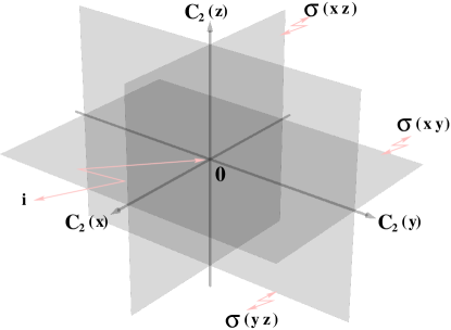
Figure 3: The symmetry elements of the two particles interacting by a central potential in a $\sin^{2}$-like trap. The list is complete with the identity element E added.

The symmetry group D_2h has eight irreducible representations (see Table 1): $A_{g}$, $B_{1g}$, $B_{2g}$, $B_{3g}$, $A_{u}$, $B_{1u}$, $B_{2u}$, $B_{3u}$. Clearly, the explicit use of symmetry is advantageous, since it reduces the numerical efforts dramatically as the different irreducible representations can be treated independently of each other. This reduces the dimensions of the matrices that have to be diagonalized by approximately a factor of $8\times 8=64$. Furthermore, many integrals vanish for symmetry reasons and have thus not to be calculated at all.

Table 1: Character table of the D_2h point group

D2h	$E$	$C_{2}(z)$	$C_{2}(y)$	$C_{2}(x)$	i	$\sigma(xy)$	$\sigma(xz)$	$\sigma(yz)$
$A_{g}$	1	1	1	1	1	1	1	1
$B_{1g}$	1	1	-1	-1	1	1	-1	-1
$B_{2g}$	1	-1	1	-1	1	-1	1	-1
$B_{3g}$	1	-1	-1	1	1	-1	-1	1
$A_{u}$	1	1	1	1	-1	-1	-1	-1
$B_{1u}$	1	1	-1	-1	-1	-1	1	1
$B_{2u}$	1	-1	1	-1	-1	1	-1	1
$B_{3u}$	1	-1	-1	1	-1	1	1	-1

In fact, the D_2h symmetry is a consequence of the considered shape of the potential and thus the symmetry of the single-particle Hamiltonians in absolute Cartesian coordinates, $\hat{\rm\mathcal{H}}_{j}$ in Eq. (2). Since the atom-atom interaction $\hat{\rm u}$ is invariant under all operations in D_2h, the total Hamiltonian $\hat{\rm\mathcal{H}}$ in Eq. (1) belongs also to the D_2h group. As may be less transparent on a first glance, but can be shown from a complete symmetry analysis, also the rel. and c.m. Hamiltonians $\hat{\rm h}_{\rm rel.}(\vec{r})$ and $\hat{\rm h}_{\rm c.m.}(\vec{R})$ possess the same symmetry as the total Hamiltonian. Therefore, it is sufficient to examine the symmetry properties, e. g., for the rel. part only. The c.m. part has the same properties and the ones of the total Hamiltonian can then be deduced from the properties of the direct tensor products.

Table 2: Results of the D_2h group operations on the absolute and spherical coordinates, and the corresponding transformations of spherical harmonics. Given are the values of $a,\,b,\,c$ that are multipliers for the $x,\,y,\,z$ coordinates, respectively, and $\theta^{\prime},\,\phi^{\prime}$ that are shifts of the spherical coordinates $\theta,\,\phi$, respectively.

symmetry	Absolute	Spherical	$Y_{l}^{m}$
	$(a\,x,b\,y,c\,z)$	($\theta^{\prime}+\theta$, $\phi^{\prime}+\phi$)	$Y_{l}^{m}(\theta^{\prime}+\theta,\phi^{\prime}+\phi)$
E	$(1,1,1)$	($0+\theta,0+\phi$)	$Y_{l}^{m}(\theta,\phi)$
$C_{2}(z)$	$(-1,-1,1)$	$(0+\theta,\pi+\phi)$	$(-1)^{m}\,Y_{l}^{m}(\theta,\phi)$
$C_{2}(y)$	$(-1,1,-1)$	$(\pi-\theta,\pi-\phi)$	$(-1)^{l+m}\,Y_{l}^{-m}(\theta,\phi)$
$C_{2}(x)$	$(1,-1,-1)$	$(\pi-\theta,2\pi-\phi)$	$(-1)^{l}\,Y_{l}^{-m}(\theta,\phi)$
i	$(-1,-1,-1)$	($\pi-\theta,\pi+\phi$)	$(-1)^{l}\,Y_{l}^{m}(\theta,\phi)$
$\sigma(xy)$	$(1,1,-1)$	$(\pi-\theta,0+\phi)$	$(-1)^{l+m}\,Y_{l}^{m}(\theta,\phi)$
$\sigma(xz)$	$(1,-1,1)$	$(0+\theta,2\pi-\phi)$	$(-1)^{m}\,Y_{l}^{-m}(\theta,\phi)$
$\sigma(yz)$	$(-1,1,1)$	($0+\theta,\pi-\phi$)	$Y_{l}^{-m}(\theta,\phi)$

In order to use the symmetry when solving the eigenvalue problems of the uncoupled rel. and c.m. motions, symmetry-adapted basis functions have to be obtained. Since all basis functions adopted in this work are centered at the origin and are products of a radial part times a spherical harmonic, (53) and (55), the symmetry operations affect only the angular part. Therefore, linear combinations of the spherical harmonics have to be found that transform like the irreducible representations of the D_2h group. The problem of determining symmetry-adapted basis functions from the complete set of spherical harmonics has a long history, starting with the introduction of cubic harmonics for the cubic point group von der Lage and Bethe (1947). Since it appears, however, to be not that trivial to find the orthorhombic harmonics in easily accessible form, they are given explicitly together with a brief derivation. First, the action of the symmetry elements of D_2h on the spherical harmonics has to be considered. The result is shown in Table 2 that provides also the intermediate steps, the result of applying the symmetry operations on the Cartesian and the spherical coordinates. The most important result is that all symmetry operations of D_2h leave $l$ unchanged, i. e., only $Y_{l}^{m}$ with identical values of $l$ are transformed into each other. As a consequence, the symmetry-adapted basis functions are superpositions of spherical harmonics with a fixed value of $l$.

In view of the eight irreducible representations of D_2h (see Table 1) one needs to find the required eight sets of orthonormal linear combinations of spherical harmonics. In the present case, this is easily achieved using the standard projector technique, i. e., by applying the projector

$$\hat{\rm P}_{i}=\frac{1}{h}\sum_{k=1}^{h}\>\chi_{i}(\hat{\rm O}_{k})^{*}\,\hat{\rm O}_{k}$$ (76)

of the irreducible representation $i$ onto a spherical harmonic $Y_{l}^{m}$. In Eq. (76) it is used that all irreducible representations in D_2h are non-degenerate. Furthermore, $h$ is the total number of symmetry operations (eight for D_2h), $\hat{\rm O}_{k}$ the operator corresponding to symmetry element $k$, and $\chi_{i}(\hat{\rm O}_{k})$ the character of symmetry element $k$ for the irreducible representation $i$. While all characters are listed in Table 1, the results of the symmetry operations on $Y_{l}^{m}$ are given in the last column of Table 2. For example, the application of $\hat{\rm P}_{B_{3u}}$ gives

$$\hat{\rm P}_{B_{3u}}\,Y_{l}^{m}=\frac{1}{8}\>\left[\,1-(-1)^{m}-(-1)^{l}+(-1)^{l+m}\,\right]\>Y_{l}^{m}{}\\ {}\>+\>\left[\,(-1)^{l}-(-1)^{l+m}+(-1)^{m}-1\,\right]\>Y_{l}^{-m}\,.$$ (77)

Clearly, only the combination of odd values of $l$ and $m$ yields in this case a non-zero result and thus a symmetry-adapted basis function,

$$\hat{\rm P}_{B_{3u}}\,Y_{l}^{m}=\frac{1}{2}\>\left(\,Y_{l}^{m}-Y_{l}^{-m}\,\right)\qquad l,m\quad{\rm odd}\,.$$ (78)

The use of these symmetry-adapted basis functions (superposition of spherical harmonics instead of a single one and restriction on $l$ and $m$) modifies the wave functions of the rel. motion in Eq. (53) into

$$\varphi_{i}^{A_{g}} = \sum\limits_{\alpha=1}^{N_{r}}\sum\limits_{l=0,\{2\}}^{N_{l}}\sum\limits_{m=0,\{2\}}^{l}\tilde{c}_{i,\alpha lm}^{A_{g}}\,r^{-1}\,B_{\alpha}(r)\mathscr{Y}_{lm}^{+}$$ (79)

$$\varphi_{i}^{B_{1g}} = \sum\limits_{\alpha=1}^{N_{r}}\sum\limits_{l=2,\{2\}}^{N_{l}}\sum\limits_{m=2,\{2\}}^{l}\tilde{c}_{i,\alpha lm}^{B_{1g}}\,r^{-1}\,B_{\alpha}(r)\mathscr{Y}_{lm}^{+}$$ (80)

$$\varphi_{i}^{B_{2g}} = \sum\limits_{\alpha=1}^{N_{r}}\sum\limits_{l=2,\{2\}}^{N_{l}}\sum\limits_{m=1,\{2\}}^{l}\tilde{c}_{i,\alpha lm}^{B_{2g}}\,r^{-1}\,B_{\alpha}(r)\mathscr{Y}_{lm}^{-}$$ (81)

$$\varphi_{i}^{B_{3g}} = \sum\limits_{\alpha=1}^{N_{r}}\sum\limits_{l=2,\{2\}}^{N_{l}}\sum\limits_{m=1,\{2\}}^{l}\tilde{c}_{i,\alpha lm}^{B_{3g}}\,r^{-1}\,B_{\alpha}(r)\mathscr{Y}_{lm}^{+}$$ (82)

$$\varphi_{i}^{A_{u}} = \sum\limits_{\alpha=1}^{N_{r}}\sum\limits_{l=3,\{2\}}^{N_{l}}\sum\limits_{m=2,\{2\}}^{l}\tilde{c}_{i,\alpha lm}^{A_{u}}\,r^{-1}\,B_{\alpha}(r)\mathscr{Y}_{lm}^{-}$$ (83)

$$\varphi_{i}^{B_{1u}} = \sum\limits_{\alpha=1}^{N_{r}}\sum\limits_{l=1,\{2\}}^{N_{l}}\sum\limits_{m=0,\{2\}}^{l}\tilde{c}_{i,\alpha lm}^{B_{1u}}\,r^{-1}\,B_{\alpha}(r)\mathscr{Y}_{lm}^{+}$$ (84)

$$\varphi_{i}^{B_{2u}} = \sum\limits_{\alpha=1}^{N_{r}}\sum\limits_{l=1,\{2\}}^{N_{l}}\sum\limits_{m=1,\{2\}}^{l}\tilde{c}_{i,\alpha lm}^{B_{2u}}\,r^{-1}\,B_{\alpha}(r)\mathscr{Y}_{lm}^{+}$$ (85)

$$\varphi_{i}^{B_{3u}} = \sum\limits_{\alpha=1}^{N_{r}}\sum\limits_{l=1,\{2\}}^{N_{l}}\sum\limits_{m=1,\{2\}}^{l}\tilde{c}_{i,\alpha lm}^{B_{3u}}\,r^{-1}\,B_{\alpha}(r)\mathscr{Y}_{lm}^{-}$$ (86)

where

$$\mathscr{Y}_{l0}^{+} = \mathscr{Y}_{l0}^{-}=Y_{l}^{0}(\theta,\phi)\,,$$ (87)

$$\mathscr{Y}_{lm}^{\pm} = Y_{l}^{m}(\theta,\phi)\pm Y_{l}^{-m}(\theta,\phi)\quad(m\neq 0)$$ (88)

is introduced for compactness and a summation index $l=i,\{2\}$ means $l=i,i+2,\dots$ Moreover, for the coefficients $\tilde{c}$ the superscripts rel. are omitted for better readability. Clearly, the consideration of symmetry-adapted basis functions for the c.m. motion leads to a completely analogous modification of Eq. (55).

Table 3: Product table of the D_2h point group

$\otimes$	$A_{g}$	$B_{1g}$	$B_{2g}$	$B_{3g}$	$A_{u}$	$B_{1u}$	$B_{2u}$	$B_{3u}$
$A_{g}$	$A_{g}$	$B_{1g}$	$B_{2g}$	$B_{3g}$	$A_{u}$	$B_{1u}$	$B_{2u}$	$B_{3u}$
$B_{1g}$	$B_{1g}$	$A_{g}$	$B_{3g}$	$B_{2g}$	$B_{1u}$	$A_{u}$	$B_{3u}$	$B_{2u}$
$B_{2g}$	$B_{2g}$	$B_{3g}$	$A_{g}$	$B_{1g}$	$B_{2u}$	$B_{3u}$	$A_{u}$	$B_{1u}$
$B_{3g}$	$B_{3g}$	$B_{2g}$	$B_{1g}$	$A_{g}$	$B_{3u}$	$B_{2u}$	$B_{1u}$	$A_{u}$
$A_{u}$	$A_{u}$	$B_{1u}$	$B_{2u}$	$B_{3u}$	$A_{g}$	$B_{1g}$	$B_{2g}$	$B_{3g}$
$B_{1u}$	$B_{1u}$	$A_{u}$	$B_{3u}$	$B_{2u}$	$B_{1g}$	$A_{g}$	$B_{3g}$	$B_{2g}$
$B_{2u}$	$B_{2u}$	$B_{3u}$	$A_{u}$	$B_{1u}$	$B_{2g}$	$B_{3g}$	$A_{g}$	$B_{1g}$
$B_{3u}$	$B_{3u}$	$B_{2u}$	$B_{1u}$	$A_{u}$	$B_{3g}$	$B_{2g}$	$B_{1g}$	$A_{g}$

Since the D_2h point group contains only non-degenerate irreducible representations, its product table (showing the result of a direct tensor product between a pair of irreducible representations and given in Tab. 3) is straightforwardly obtained and every product corresponds uniquely to one irreducible representation. For example, a configuration $\Phi_{\kappa}=\varphi_{i_{\kappa}}^{B_{3g}}\,\psi_{j_{\kappa}}^{B_{2g}}$ transforms as $B_{1g}$. Clearly, symmetry-adapted configurations are straightforwardly constructed from the symmetry-adapted rel. and c.m. orbitals.

In the case of indistinguishable atoms, the quantum statistics has to be considered. For Fermionic atoms, the total wavefunction must change sign under particle exchange, while it must remain the same for Bosons. Particle exchange does not influence the c.m. coordinate (i. e., $\vec{R}\rightarrow\vec{R}$ or, equivalently, $\Phi\rightarrow\Phi,\,\Theta\rightarrow\Theta$), but the rel. coordinate (i. e., $\vec{r}\rightarrow-\vec{r}$ or $\phi\rightarrow\pi+\phi,\,\theta\rightarrow\pi-\theta$). Since particle exchange corresponds to the symmetry operation of inversion (i) for the coordinate, all gerade basis functions ($\varphi_{A_{g}}$, $\varphi_{B_{1g}}$, $\varphi_{B_{2g}}$, and $\varphi_{B_{3g}}$) are allowed for identical Bosons, the ungerade functions ($\varphi_{A_{u}}$, $\varphi_{B_{1u}}$, $\varphi_{B_{2u}}$, and $\varphi_{B_{3u}}$) for identical Fermions. The quantum statistics for indistinguishable atoms is thus easily taken into account and reduces the number of possible orbital combinations by factor 2. The straightforward (almost automatic) implementation of the quantum statistics that leads even to a direct reduction of the computational demands is a further advantage of the present approach.

V Computational details

The theoretical approach presented in this work provides an efficient way to treat two interacting atoms in an orthorhombic optical lattice. The use of c.m. and rel. coordinates and the expansion of the basis functions in $B$ splines for the radial part and spherical harmonics for the angular parts is especially useful for considering realistic interatomic (molecular) interaction potentials. Furthermore, the Bosonic or Fermionic nature of the atoms is easily accounted for. However, in the case of strongly anisotropic lattice potentials the advantage of the use of spherical harmonics that all involved integrals can be efficiently and analytically calculated is partly compensated by their slow convergence. Similarly, the adopted exact diagonalization approach for incorporating the coupling of c.m. and rel. motion has the advantage of being exact, if converged, but is known to be slowly convergent. For many experimentally relevant parameters the calculations are, therefore, still very demanding and thus an efficient implementation of all involved computational steps was mandatory. The adequate choice of the basis-set parameters adapted to the considered problem can improve the efficiency drastically. Thus it is worthwhile to at least briefly discuss some technical aspects of both the implementation and the choice of basis sets.

V.1 Interatomic interaction potential

In the present approach the interatomic interaction enters the calculation only in the determination of the rel. orbitals. In the so far considered case of isotropic interaction potentials the potential influences only the calculation of the radial integral (68). Clearly, an extension to orientation-dependent interaction potentials (like dipole-dipole interaction) is possible by expanding the angular part of the interaction potential in spherical harmonics. Then the resulting angular integrals can still be solved analytically. Since the radial integral (68) is calculated using quadrature, even a usually only numerically given Born-Oppenheimer potential curve can be used in order to achieve a realistic description of the interatomic interaction. Clearly, any type of potential can be easily used. Only the implementation of the $\delta$-function pseudopotential required some care due to its numerically ill-behaved nature.

In the ultracold regime the scattering process is extremely sensitive to all details of the complete interatomic potential curve. In fact, for most experimentally relevant alkali atoms, it is impossible to calculate the potential curves with sufficient precision. In the zero-energy limit the scattering process is fully described by the scattering length $a_{\rm sc}$ Weiner et al. (1999). Depending on the considered atoms, their isotopes, and electronic states $a_{\rm sc}$ can have very different values for different systems, ranging from $a_{\rm sc}\gg 0$ (strongly repulsive) via $a_{\rm sc}\approx 0$ (almost non-interacting) to $a_{\rm sc}\ll 0$ (strongly attractive). An important aspect of ultracold atomic gases is the fact that many atom pairs possess magnetic Feshbach resonances, i. e., with a magnetic field the colliding atoms can be brought into resonance with a molecular bound state. As a consequence, the scattering length becomes experimentally tunable Loftus et al. (2002); Regal and Jin (2003). This method was also successfully used to tune the interatomic interaction between atoms in the optical lattices, see, e. g., Köhl et al. (2005); Stöferle et al. (2006); Ospelkaus et al. (2006).

However, the correct theoretical treatment of a magnetic Feshbach resonance requires the solution of a multichannel problem that is numerically demanding due to the different length scales involved. Within an optical lattice the influence of the confining potential on the multichannel problem has also to be properly considered (see Schneider et al. (2011) and references therein). To perform such a study within the present algorithm appears prohibitively difficult, at least with the computer resources at our disposal. On the other hand, the variation of the interaction strength (characterized in the trap-free situation and at the zero-energy limit by $a_{\rm sc}$) can be mimicked within single-channel models. In this case, some parameter in the rel. motion Hamiltonian is varied in such a fashion that resonant behavior occurs. Whenever the manipulation leads to a shift of a very weakly bound state into the dissociation continuum, resonant behavior (divergence of $a_{\rm sc}$) is observed. Examples for such artificially obtained single-channel resonances include the variation of van der Waals coefficients Ribeiro et al. (2004), the reduced mass Grishkevich and Saenz (2007), the inner-wall of the molecular interaction potential Grishkevich and Saenz (2009), or the local modification of the Born-Oppenheimer curve at intermediate distances Grishkevich et al. (2010). A comparison of these different procedures and the full multi-channel treatment is provided in Grishkevich et al. (2010). As is shown in Schneider et al. (2009) a better and in fact almost perfect model for a multi-channel Feshbach resonance can be obtained with a two-channel model which appears more realistic with respect to a possible implementation within the present approach than the full multi-channel Hamiltonian.

V.2 Basis-set considerations

Due to the choice of spherical c.m. and rel. coordinates all integrals could be reduced to products of one-dimensional integrals that can be solved very accurately and efficiently. In fact, the angular integrations are performed analytically. Moreover, the Gaussian quadrature provides exact results for all radial integrals except the ones of the interatomic interaction. However, even the latter ones can be calculated to high precision using Gaussian quadrature. The compactness of the $B$ splines leads to sparseness of the Hamiltonian matrices, since only few integrals involve two non-zero $B$ splines. The compactness and thus the resulting band structure of the one-particle Hamiltonian matrices (of c.m. and rel. motion) is controlled by the order $k_{\rm rel.}$ and $k_{\rm c.m.}$ of the $B$ splines. A higher order leads to a broader band structure, but it offers also a higher flexibility of the basis functions, since it corresponds to a polynomial of higher order. Thus less $B$ splines are needed for a comparable result, if a higher order is adopted. Usually, the orders of $k_{\rm rel.}$ ($k_{\rm c.m.}$) of 8 or 9 turn out to be the best compromise with respect to basis-set size and sparseness, but also with respect to numerical stability in view of the finite precision in which floating-point numbers are stored in the computer.

The two other parameters defining the radial $B$-spline basis are the number of $B$ splines and their knot sequence. Clearly, the computational efforts (number of integrals that have to be calculated and size of the matrices that have to be diagonalized) depend crucially on the number of $B$ splines. Since more $B$ splines are required for describing highly oscillatory wavefunctions, it is most efficient to use non-uniform knot sequences in which the $B$-spline density is higher in the highly oscillatory regions of (radial) space.

In the context of ultracold collisions the energetically low-lying c.m. orbitals $\psi(\vec{R}\,)$ are the ones that usually are of main interest. Since they possess only a small number of nodes (none in the lowest state), the demands on the $B$-spline basis are not too high. For the simplest case of a single-well lattice potential $N_{R}=50$ to $N_{R}=100$ $B$ splines (or even less) were found to be sufficient to obtain convergence for the ground and lowest-lying excited states of the c.m. motion Grishkevich and Saenz (2009). Also the lowest-lying states in a more structured trap potential like the triple-well potential considered in Schneider et al. (2009) were satisfactorily treated with 70 $B$ splines. A linear knot sequence is usually adequate in this case.

The description of the rel. orbitals $\varphi(\vec{r}\,)$ is more demanding, since one is usually not interested in the lowest-lying, deeply bound molecular states, but in the most weakly bound states or the low-lying dissociative ones. The Born-Oppenheimer potentials of alkali-metal atom dimers support often a large number of bound states Grishkevich and Saenz (2007). The very long-ranged, weakly bound states consist, therefore, of a highly oscillatory inner part (covering the molecular regime and providing the orthogonality to all lower lying bound states) and a rather smooth long-range part. Hence, it is advantageous to distribute a majority of $B$ splines in the molecular range of the potential while they are a sparser distributed in the outer part. The distribution of the B splines is given by the knot sequence $\{r_{i}\}$, $i=1,2,\dots$ specifying a continuous chain of segments on which the $B$-spline functions are defined. The choice of a combined linear and geometrical knot sequence Vanne and Saenz (2004) for describing the short and long-range parts, respectively, has proven to be very efficient also in the present context Grishkevich and Saenz (2009). The linear distribution of the knot sequence is given by

$$r_{i+k_{\rm rel.}}=\rho_{\rm min.}+i\,s,\quad i=1,2,...,N_{r}^{\rm lin.}-k_{\rm rel.}$$ (89)

where $N_{r}^{\rm lin.}$ and $\rho_{\rm min.}$ are the number of $B$ splines in the linear interval and the origin of the linear interval, respectively. Furthermore, $s$ is the linear step size, i.e., the distance between neighboring knots given as

$$s=\frac{\rho_{\rm lin.}-\rho_{\rm min.}}{N_{r}^{\rm lin.}-k_{\rm rel.}+1}\,.$$ (90)

Owing to the steep inner-wall of the molecular potential the wave function $\varphi_{i}(r)$ vanishes well before $r=0$. Therefore, $\rho_{\rm min.}$ is usually taken non-zero in order to save on the number of $B$ splines. The exact value of $\rho_{\rm min.}$ depends on the potential of the considered electronic state. Note, $k_{r}$ points must be placed at both ends of the box in accordance with the definition of $B$ splines on the knot sequence (e.g., $r_{1}=r_{2}=...=r_{k_{\rm rel.}}=\rho_{\rm min.}$). The linear step $s$ is taken as the scale factor for the geometric progression to ensure the smooth distribution of $B$ splines at the border of the linear and geometric zones. In the geometrical knot sequence the separation of the knot points increases (according to a geometric series) with increasing distance. It is given by

$$r_{i+N_{r}^{\rm lin.}}=\rho_{\rm lin.}+s\,q^{i-1},\quad i=1,...,N_{r}^{\rm geo.}$$ (91)

where $N_{r}^{\rm geo.}$ is the number of $B$ splines in the geometric interval and $q$ is the common ratio for the geometric progression defined as

$$q=\left(\frac{\rho_{\rm box.}-\rho_{\rm lin.}}{s}\right)^{\displaystyle\frac{1}{N_{r}^{\rm geo.}-1}}\,.$$ (92)

The last parameter is the maximum value of angular momentum $l_{\rm max}$ used and thus the number of angular basis functions. Clearly, a more spherical-like lattice potential needs less angular momenta for representing the orbitals. The worst case is a highly anisotropic lattice geometry, since the spherical-harmonic basis converges extremely slowly in such a case. While a small value of $l_{\rm max}$ of 1 or 2 was sufficient to obtain converged orbitals for an isotropic (cubic) single-well potential in Grishkevich and Saenz (2009) in which among others also the experiment in Ospelkaus et al. (2006) was successfully modeled and thus realistic parameters were adopted. On the other hand, the much more anisotropic triple-well potential considered in Schneider et al. (2009) required $l_{\rm max}=32$ for converged orbitals.

V.3 Example of a very anisotropic trap

Since a highly anisotropic lattice geometry provides a great challenge to our approach, it is important to demonstrate that even such a problem can be handled satisfactorily. Another motivation is the present interest in ultracold atomic systems of reduced dimensionality. Using strong confinement along one or two orthogonal directions, quasi one- or two-dimensional structures can nowadays be produced in the lab. Such systems show remarkable quantum properties not encountered in three dimensions. A major experimental breakthrough was the realization of Tonk-Girardeau gases of Bosons with strongly repulsive interaction Girardeau (1960); Paredes et al. (2004). Being placed in 1D and repelling each other Bosons are hindered from occupying the same position in space. This mimics the Pauli exclusion principle for Fermions, causing the Bosonic particles to exhibit Fermionic properties. Another peculiar property of reduced dimensionality systems is the occurrence of confinement-induced resonances that were recently experimentally observed Haller et al. (2010); Fröhlich et al. (2011). Confinement-induced 1D Feshbach resonances reachable by tuning the 1D coupling constant via 3D Feshbach scattering resonances occur for both Bose gases Olshanii (1998) and spin-aligned Fermi gases Granger and Blume (2004). Near a confinement-induced resonances, the effective 1D interaction is very strong, leading to strong short-range correlations, breakdown of effective field theories, and emergence of a highly correlated ground state. Although confinement-induced resonances were originally predicted to occur already when only the rel. motion is considered Olshanii (1998); Petrov et al. (2000); Bergeman et al. (2003), it was recently shown and furthermore verified using the here presented numerical approach that the ones observed in Haller et al. (2010) are in fact caused by the coupling of the c.m. and rel. degrees of freedom Sala et al. (2011).

A typical system to study effects of low dimensionality is two atoms confined in a quasi 1D cigar-shaped harmonic trap. We adopt this two-body setup to probe the quality of the present computational method in an extreme case of the strong anisotropic confinement. As was already mentioned, if the interparticle interaction between atoms is modeled by the $\delta$-function pseudopotential the problem can be solved analytically. Therefore, the numerical results can be compared with the predictions of the pseudopotential model. One-dimensional external confinement is prepared by setting a strong harmonic frequency in either of two spatial directions, e. g., $\omega_{x}=\omega_{y}\gg\omega_{z}$ where $\omega_{i}$ stands for the harmonic oscillator frequency along the spatial direction $i$. It is worthwhile to note that the analytical solution is only known for this special case of the single anisotropy Liang and Zhang (2008). This emphasizes the need for numerical approaches to calculate spectra in totally anisotropic confinement where $\omega_{x}\neq\omega_{y}\gg\omega_{z}$.

The Hamiltonian of two identical particles in our harmonic trap separates in rel. and c.m. motion. The c.m. spectrum reduces to the one of a simple harmonic oscillator. This simplifies the problem to calculate the rel. spectrum. Hence, it is sufficient to solve numerically Eq. (50) only. In the following two Bosonic ⁷Li atoms are considered that are placed in the prolate trap with $\omega_{x}=\omega_{y}=10\,\omega_{z}$ and interacting via the potential of the $a^{3}\Sigma_{g}^{+}$ electronic triplet state. This electronic state has the advantage of supporting a small number of bound states. Therefore, a smaller number of $B$ splines is required to reproduce the $\varphi_{i}(\vec{r})$ functions. The numerical data for the Born-Oppenheimer potential curve are adopted from Grishkevich and Saenz (2007). In order to achieve converged results for the first few states $l_{\rm max}=30$, a box size of approximately $\rho_{\rm box}\approx 5\times 10^{4}a_{0}$, where $a_{0}$ is the Bohr radius, and $N_{r}=100$ $B$ splines of the order $k_{\rm rel.}=8$ were used. Half of the $B$ splines ($N_{r}^{\rm lin.}=50$) are distributed linearly according to Eq. (89) over the small interatomic distance of $\rho_{\rm lin.}=15\,a_{0}$ to reproduce the highly oscillatory structure of $\varphi_{i}(r)$ in this region. Furthermore, for our calculations we can safely choose $\rho_{\rm min.}=2\,a_{0}$. The remaining $B$ splines ($N_{r}^{\rm geo.}=50$) are distributed in an ascending geometric progression according to Eq. (91) over the residual interval. Finally, different values of the interaction strength are obtained using a single-channel approach by a smooth variation of the inner wall of the molecular interaction potential Grishkevich et al. (2010). Figure 4 shows the calculated spectrum of the rel. Hamiltonian together with the analytical prediction of the pseudopotential approximation. The spectral curves are plotted as functions of $d_{x}/a_{\rm sc}$, where $d_{x}=\sqrt{\hbar/(\mu\,\omega_{x})}$ is the harmonic oscillator length in transversal direction.

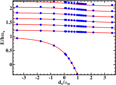
Figure 4: Energy spectrum of two Bosonic atoms confined in a harmonic trap of anisotropy ${\omega_{x}}/{\omega_{z}}=10$. The numerical calculation (blue dots) is compared to the analytical prediction of the pseudopotential approximation (red lines).

As is evident from Fig. 4, the first four trap states and the bound state match perfectly with the analytical prediction of the pseudopotential model. However, high lying states show deviations.

In order to explain the increasing mismatch found for higher lying states and to give an impression of the convergence behavior of the present approach, energy spectra for different values of the angular momentum are calculated. For the calculations $d_{x}/a_{\rm sc}=1.46$ is chosen. Close to this value a confinement-induced resonance should occur Olshanii (1998) motivating this choice. The results of the calculations are shown in Fig. 5. As is seen from this figure, at $l_{\rm max}=30$ the slopes of the energy curves are approximately zero, especially for the first four trap states. This indicates that convergence is achieved with respect to $l_{\rm max}$. Figure 5 clearly demonstrates that the high lying states require larger values of the angular momentum for convergence. This can now as well be concluded from Fig. 4.

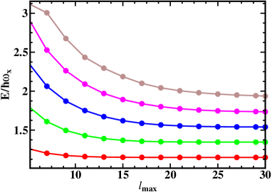
Figure 5: The energy of the first five trap states for different values of $l_{\rm max}$ in the strongly repulsive regime for $d_{x}/a_{\rm sc}=1.46$. The deeper lying bound state is not shown here, because it is already converged for $l_{\rm max}=5$. (To guide the eye, the discrete points of the numerical calculation are connected by continuous lines.)

While convergence can be extended to higher energies or higher anisotropies by increasing $l_{\rm max}$, the computational efforts increase adding new angular momenta. However, as the precision is only limited by hardware capacities, this example demonstrates the applicability of the approach even for extreme setups.

V.4 Exact diagonalization (configuration interaction)

The demands of the exact diagonalization also known as configuration interaction (CI) depend evidently again on the physical system under consideration. While the atom-atom interaction is very efficiently handled even for strongly interacting atoms and basically contained in the rel. orbitals, the CI takes care of the c.m. and rel. coupling. Thus its convergence depends on the strength of this coupling. Correspondingly, convergence is much faster for weakly coupled systems. If all configurations that can be built with the c.m. and rel. orbitals are included, full CI is achieved. While being well defined, full CI scales very inconveniently with the number of orbitals. Therefore, it is in practice in most cases more advantageous to include only a limited number of the possible configurations. For example, the inclusion of the orbitals of very high energy does usually not lead to a noticeable improvement of the low lying states. Therefore, an energy cut-off may be introduced in the orbital selection. If the interest is mainly on those states that are weakly bound or dissociative, but close to the dissociation threshold, the deeply bound molecular states can be omitted from the CI configurations Grishkevich and Saenz (2009). Note, however, that a good representation of those states in the calculation of the rel. orbitals is nevertheless important, since otherwise the rel. orbitals of the weakly bound states are not well described and this can in practice not be compensated by the CI calculation. In the worst case the calculation of the rel. orbitals provides too few bound states and then the nodal structure of the weakly bound states is evidently wrong.

Although the coupled Hamiltonian matrices are usually much larger than the uncoupled ones and are therefore harder to diagonalize, there are two points easing the treatment of the coupled ones. First, the eigenvalue problem to be solved in the CI step is a standard one (meaning that the the basis is orthonormal), while generalized ones occur in the orbital calculations. Second, in many cases only a relatively small number of CI states is required. Therefore, it is possible to use Lanzcos or Davidson type diagonalization routines that (iteratively) provide a small number of eigenstates within a specific energy interval. Here we adopted the Davidson-based diagonalization routine JADAMILU Bollhöfer and Notay (2007) that is especially designed for the efficient diagonalization of large sparse matrices.

Finally, it should be noted that the choice of expressing all wavefunctions in rel. and c.m. coordinates is advantageous for computational reasons, but often not very helpful in the interpretation of the results. Especially in the case of multi-well potentials the obtained wavefunctions and densities are often very complicated. Therefore, a further code was implemented that allows the application of the inverse coordinate transform from c.m.-rel. coordinates to the absolute ones according to $\displaystyle\vec{r}_{1}=\vec{R}+\mu_{2}\vec{r}$ and $\displaystyle\vec{r}_{2}=\vec{R}-\mu_{1}\vec{r}$ to the wavefunctions, especially to $\Psi(\vec{R},\vec{r})$ which allowed a much easier physical interpretation, e. g., in Grishkevich and Saenz (2009).

VI Summary and outlook

An approach that allows the full numerical description of two ultracold atoms in a finite orthorhombic 3D optical lattice is presented. The coupling between center-of-mass and relative motion coordinates is incorporated in a configuration-interaction manner and hence the full 6D problem is solved. An important feature is the use of realistic interatomic interaction potentials adopting, e. g., numerically provided Born-Oppenheimer curves. The use of spherical harmonics together with $B$ splines as basis functions and the expansion of the trap in terms of spherical harmonics leads to an analytical form of the matrix elements, except those of the interparticle interaction, if the interaction potential is defined only numerically. The sparseness of the Hamiltonian matrices due to the use of the compact radial $B$-spline basis is considered explicitly. This makes the method computationally efficient. Additionally, the lattice symmetry and a possible indistinguishability of the atoms (Bosonic or Fermionic statistics) is considered explicitly. This simplifies the calculations and helps to interpret the solutions.

The here presented approach has already proven its applicability by considering the influence of the anharmonicity in a single site of an optical lattice in Grishkevich and Saenz (2009) where a corresponding experiment Ospelkaus et al. (2006) could be reproduced and analyzed. The validity range of the Bose-Hubbard model together with an improved determination of the Bose-Hubbard parameters was investigated considering a triple-well potential in Schneider et al. (2009).

The implemented approach was formulated in a rather general way in order to allow extensions in various directions. Since the optical-lattice potential is (via the Taylor expansion) expressed as a superposition of polynomials, it is rather straightforward to consider other than pure $\sin^{2}$ or $\cos^{2}$ potentials, as long as they can be represented with (a reasonable number of) polynomials. This includes tilted lattices and superlattices. Care has, however, to be taken that the orthorhombic symmetry is either preserved, or new symmetry rules have to be implemented.

Substitution of the numerical interatomic potential by, e. g., the Coulomb potential allows to describe either two electrons or an exciton in quantum-dot atoms or molecules. It is furthermore planned to implement non-isotropic interatomic potentials like dipole-dipole interactions as they are of interest for Cr or Rydberg atoms and for heteronuclear diatomic molecules. Finally, an extension of the approach in the direction of time-dependent problems (with time dependent lattice or interatomic interaction potentials) is currently under way.

References

- Anderson et al. (1995) M. H. Anderson, J. R. Ensher, M. R. Matthews, C. E. Wieman, and E. A. Cornell, Science 269, 198 (1995).
- Davis et al. (1995) K. B. Davis, M. O. Mewes, M. R. Andrews, N. J. van Druten, D. S. Durfee, D. M. Kurn, and W. Ketterle, Phys. Rev. Lett. 75, 3969 (1995).
- Jaksch et al. (1998) D. Jaksch, C. Bruder, J. I. Cirac, C. W. Gardiner, and P. Zoller, Phys. Rev. Lett. 81, 3108 (1998).
- Greiner et al. (2002) M. Greiner, O. Mandel, T. Esslinger, T. Hänsch, and I. Bloch, Nature 415, 39 (2002).
- Köhl et al. (2005) M. Köhl, H. Moritz, T. Stöferle, K. Günter, and T. Esslinger, Phys. Rev. Lett. 94, 080403 (2005).
- Meacher (1998) D. R. Meacher, Contemp. Phys. 39, 329 (1998).
- Bloch (2005) I. Bloch, Nat. Phys. 1, 23 (2005).
- Lewenstein et al. (2007) M. Lewenstein, A. Sanpera, V. Ahufinger, B. Damski, A. Sen, and U. Sen, Adv. Phys. 56, 243 (2007).
- Bloch et al. (2008) I. Bloch, J. Dalibard, and W. Zwerger, Rev. Mod. Phys. 80, 885 (2008).
- Weiner et al. (1999) J. Weiner, V. S. Bagnato, S. Zilio, and P. S. Julienne, Rev. Mod. Phys. 71, 1 (1999).
- Loftus et al. (2002) T. Loftus, C. A. Regal, C. Ticknor, J. L. Bohn, and D. S. Jin, Phys. Rev. Lett. 88, 173201 (2002).
- Regal et al. (2003) C. A. Regal, C. Ticknor, J. L. Bohn, and D. S. Jin, Nature 424, 47 (2003).
- Hubbard (1963) J. Hubbard, Proc. R. Soc. A 276, 238 (1963).
- Simon et al. (2011) J. Simon, W. S. Bakr, R. Ma, M. E. Tai, P. M. Preiss, and M. Greiner, Nature 472, 307 (2011).
- Kraemer et al. (2006) T. Kraemer, M. Mark, P. Waldburger, J. G. Danzl, C. Chin, B. Engeser, A. D. Lange, K. Pilch, A. Jaakkola, H.-C. Nägerl, et al., Nature 440, 315 (2006).
- Valiente et al. (2010a) M. Valiente, D. Petrosyan, and A. Saenz, Phys. Rev. A 81, 011601 (2010a).
- Valiente et al. (2010b) M. Valiente, M. Küster, and A. Saenz, Europhys. Lett. 92, 10001 (2010b).
- Chatterjee et al. (2010) B. Chatterjee, I. Brouzos, S. Zöllner, and P. Schmelcher, Phys. Rev. A 82, 043619 (2010).
- DeMille (2002) D. DeMille, Phys. Rev. Lett. 88, 067901 (2002).
- Jaksch and Zoller (2004) D. Jaksch and P. Zoller, Adv. Phys. 315, 52 (2004).
- Schneider and Saenz (2011) P.-I. Schneider and A. Saenz, Quantum computation with ultracold atoms in a driven optical lattice (2011), arXiv:1103.4950.
- Bolda et al. (2005) E. L. Bolda, E. Tiesinga, and P. S. Julienne, Phys. Rev. A 71, 033404 (2005).
- Grishkevich and Saenz (2007) S. Grishkevich and A. Saenz, Phys. Rev. A 76, 022704 (2007).
- Ospelkaus et al. (2006) C. Ospelkaus, S. Ospelkaus, L. Humbert, P. Ernst, K. Sengstock, and K. Bongs, Phys. Rev. Lett. 97, 120402 (2006).
- Deuretzbacher et al. (2008) F. Deuretzbacher, K. Plassmeier, D. Pfannkuche, F. Werner, C. Ospelkaus, S. Ospelkaus, K. Sengstock, and K. Bongs, Phys. Rev. A 77, 032726 (2008).
- Grishkevich and Saenz (2009) S. Grishkevich and A. Saenz, Phys. Rev. A 80, 013403 (2009).
- Armstrong et al. (2011) J. R. Armstrong, N. T. Zinner, D. V. Fedorov, and A. S. Jensen, J. Phys. B 44, 055303 (2011).
- Schneider et al. (2009) P.-I. Schneider, S. Grishkevich, and A. Saenz, Phys. Rev. A 80, 013404 (2009).
- Milburn et al. (1997) G. J. Milburn, J. Corney, E. M. Wright, and D. F. Walls, Phys. Rev. A 55, 4318 (1997).
- Anderlini et al. (2006) M. Anderlini, J. Sebby-Strabley, J. Kruse, J. V. Porto, and W. D. Phillips, J. Phys. B 39, S199 (2006).
- Fölling et al. (2007) S. Fölling, S. Trotzky, P. Cheinet, M. Feld, R. Saers, A. Widera, T. Müller, and I. Bloch, Nature 448, 1029 (2007).
- Cheinet et al. (2008) P. Cheinet, S. Trotzky, M. Feld, U. Schnorrberger, M. Moreno-Cardoner, S. Fölling, and I. Bloch, Phys. Rev. Lett. 101, 090404 (2008).
- Sebby-Strabley et al. (2006) J. Sebby-Strabley, M. Anderlini, P. S. Jessen, and J. V. Porto, Phys. Rev. A 73, 033605 (2006).
- Trotzky et al. (2008) S. Trotzky, P. Cheinet, S. Fölling, M. Feld, U. Schnorrberger, A. M. Rey, A. Polkovnikov, E. A. Demler, M. Lukin, and I. Bloch, Science 319, 295 (2008).
- Stickney et al. (2007) J. A. Stickney, D. Z. Anderson, and A. A. Zozulya, Phys. Rev. A 75, 013608 (2007).
- Blume and Greene (2002) D. Blume and C. H. Greene, Phys. Rev. A 65, 043613 (2002).
- Busch et al. (1998) T. Busch, B.-G. Englert, K. Rzazewski, and M. Wilkens, Found. Phys. 28, 549 (1998).
- Idziaszek and Calarco (2005) Z. Idziaszek and T. Calarco, Phys. Rev. A 71, 050701(R) (2005).
- Kohn (1959) W. Kohn, Phys. Rev. 115, 809 (1959).
- Gradshteyn and Ryzhik (2007) I. Gradshteyn and I. Ryzhik, Table of Integrals, Series, and Products (Academic Press, 2007).
- Zöllner et al. (2008) S. Zöllner, H.-D. Meyer, and P. Schmelcher, Phys. Rev. A 78, 013621 (2008).
- de Boor (1978) C. de Boor, A Practical Guide to Splines (Springer, New York, 1978).
- Bachau et al. (2001) H. Bachau, E. Cormier, P. Decleva, J. E. Hansen, and F. Martín, Rep. Prog. Phys. 64, 1815 (2001).
- Rasch and Yu (2003) J. Rasch and A. C. H. Yu, SIAM J. Sci. Comput. 25, 1416 (2003).
- Pinchon and Hoggan (2007) D. Pinchon and P. E. Hoggan, Int. J. Quant. Chem. 107, 2186 (2007).
- von der Lage and Bethe (1947) F. C. von der Lage and H. A. Bethe, Phys. Rev. 71, 612 (1947).
- Regal and Jin (2003) C. A. Regal and D. S. Jin, Phys. Rev. Lett. 90, 230404 (2003).
- Stöferle et al. (2006) T. Stöferle, H. Moritz, K. Günter, M. Köhl, and T. Esslinger, Phys. Rev. Lett. 96, 030401 (2006).
- Schneider et al. (2011) P.-I. Schneider, Y. V. Vanne, and A. Saenz, Phys. Rev. A 83, 030701 (2011).
- Ribeiro et al. (2004) E. Ribeiro, A. Zanelatto, and R. Napolitano, Chem. Phys. Lett. 390, 89 (2004).
- Grishkevich et al. (2010) S. Grishkevich, P.-I. Schneider, Y. V. Vanne, and A. Saenz, Phys. Rev. A 81, 022719 (2010).
- Vanne and Saenz (2004) Y. V. Vanne and A. Saenz, J. Phys. B 37, 4101 (2004).
- Girardeau (1960) M. Girardeau, J. Math. Phys. 1, 516 (1960).
- Paredes et al. (2004) B. Paredes, A. Widera, V. Murg, O. Mandel, S. Fölling, I. Cirac, G. V. Shlyapnikov, T. W. Hänsch, and I. Bloch, Nature 429, 277 (2004).
- Haller et al. (2010) E. Haller, M. J. Mark, R. Hart, J. G. Danzl, L. Reichsöllner, V. Melezhik, P. Schmelcher, and H.-C. Nägerl, Phys. Rev. Lett. 104, 153203 (2010).
- Fröhlich et al. (2011) B. Fröhlich, M. Feld, E. Vogt, M. Koschorreck, W. Zwerger, and M. Köhl, Phys. Rev. Lett. 106, 105301 (2011).
- Olshanii (1998) M. Olshanii, Phys. Rev. Lett. 81, 938 (1998).
- Granger and Blume (2004) B. E. Granger and D. Blume, Phys. Rev. Lett. 92, 133202 (2004).
- Petrov et al. (2000) D. S. Petrov, M. Holzmann, and G. V. Shlyapnikov, Phys. Rev. Lett. 84, 2551 (2000).
- Bergeman et al. (2003) T. Bergeman, M. G. Moore, and M. Olshanii, Phys. Rev. Lett. 91, 163201 (2003).
- Sala et al. (2011) S. Sala, P.-I. Scheider, and A. Saenz, Confinement-induced resonances revisited (2011), arXiv:1104.1561.
- Liang and Zhang (2008) J.-J. Liang and C. Zhang, Phys. Scr. 77, 025302 (2008).
- Bollhöfer and Notay (2007) M. Bollhöfer and Y. Notay, Comp. Phys. Comm. 177, 951 (2007).