Decoherence Suppression by Cavity Optomechanical Cooling

Abstract

We consider a cavity optomechanical cooling configuration consisting of a mechanical resonator (denoted as resonator $b$) and an electromagnetic resonator (denoted as resonator $a$), which are coupled in such a way that the effective resonance frequency of resonator $a$ depends linearly on the displacement of resonator $b$. We study whether back-reaction effects in such a configuration can be efficiently employed for suppression of decoherence. To that end, we consider the case where the mechanical resonator is prepared in a superposition of two coherent states and evaluate the rate of decoherence. We find that no significant suppression of decoherence is achievable when resonator $a$ is assumed to have a linear response. On the other hand, when resonator $a$ exhibits Kerr nonlinearity and/or nonlinear damping the decoherence rate can be made much smaller than the equilibrium value provided that the parameters that characterize these nonlinearities can be tuned close to some specified optimum values.

I Introduction

The quest for quantum effects in nanomechanical devices has motivated an intense research effort in recent years Blencowe_159 ; Schwab_36 ; OConnell_697 . Experimental demonstration of quantum superposition in a nanomechanical resonator may provide an important insight into the problem of quantum to classical transition Penrose_581 ; Diosi_1165 ; Legget_R415 ; Leggett_857 ; Bose_4175 ; Bose_3204 ; Kleckner_095020 . However, in many cases the lifetime of such superposition states is too short for experimental observation since the coupling between a nanomechanical resonator and its environment typically results in rapid decoherence Zurek_0306072 ; Zurek_715 . As a case study, consider a superposition of two coherent states $\left|\alpha_{1}\right\rangle$ and $\left|\alpha_{2}\right\rangle$ of a mechanical resonator having an angular resonance frequency $\omega_{b}$ and damping rate $\gamma_{b}$. The decoherence rate of such a superposition state is given in the high temperature limit $k_{\mathrm{B}}T\gg\hbar\omega_{b}$ by Caldeira_587 ; Joos_223 ; Unruh_1071 ; Zurek_36

$$\frac{1}{\tau_{\varphi}}=4\gamma_{b}\left|\delta_{\alpha}\right|^{2}\frac{k_{\mathrm{B}}T}{\hbar\omega_{b}}\;,$$ (1)

where $\delta_{\alpha}=\alpha_{2}-\alpha_{1}$.

While Eq. (1) was derived by assuming linear response, it is well known that nonlinear response can be exploited for reduction of thermal fluctuations. One example is the technique of noise squeezing that can be employed for reducing thermal fluctuations in one of the quadratures of a mechanical resonator Rugar_699 ; Almog_078103 . Another example, which is the focus of this chapter, is the technique of optomechanical cavity cooling. This technique Braginsky_2002 ; Martin_125339 ; Wilson-Rae_075507 ; Clerk_238 ; Blencowe_236 ; Wineland_0606180 ; Marquardt_093902 ; Kimble_et_al_01 , which was first proposed as a way to enhance the detection sensitivity of gravity waves Braginsky&Manukin_67 ; Braginsky_et_al_70 , can be employed for significantly reducing the energy fluctuations of a mechanical resonator well below the equilibrium value Hohberger-Metzger_1002 ; Gigan_67 ; Arcizet_71 ; Kleckner_75 ; Corbitt_et_al_06 ; Corbitt_150802 ; Schliesser_243905 ; Harris_013107 ; Naik_193 ; Schliesser_et_al_08 ; Genes_et_al_08 ; Kippenberg&Vahala_08 ; Teufel_et_al_10 ; Teufel_1103_2144 . Cooling is achieved by coupling the mechanical resonator (denoted as resonator $b$) to an electromagnetic resonator (denoted as resonator $a$) in such a way that the effective resonance frequency of resonator $a$ becomes linearly dependent on the displacement of resonator $b$. When the parameters of the system are optimally chosen the fluctuations of resonator $b$ around steady state can be significantly reduced well below the equilibrium value by externally driving resonator $a$ with a monochromatic pump tone. In this region back-reaction due to the retarded response of the driven resonator $a$ to fluctuations of resonator $b$ acts as a negative feedback, providing thus additional damping which results in effective cooling down of resonator $b$. The success of these experiments raises the question whether similar back-reaction effects can also be efficiently employed for suppression of decoherence below the equilibrium value.

Here we study this problem by generalizing Eq. (1) for the case where cavity cooling is applied. Nonlinearity in resonator $a$ is taken into account to lowest nonvanishing order. The equations of motion of the system are obtained using the Gardiner and Collett input-output theory Gardiner_3761 ; Yurke_5054 . By linearizing these equations we derive the susceptibility matrixes of the system, which allow calculating the response of both resonators to input noise. This, in turn, allows evaluating both, the spectral density of fluctuations and the decoherence rate $1/\tau_{\varphi}$ of resonator $b$. In both cases we examine the cooling efficiency by defining an appropriate effective temperature and by calculating it for an optimum choice of the system’s parameters. We find that only modest suppression of decoherence is possible using cavity cooling unless the system is driven into the region of nonlinear oscillations.

II The Model

The model consists of two resonators, labeled as $a$ and $b$ respectively, which are coupled to each other by a term $\hbar\Omega N_{a}\left(A_{b}+A_{b}^{{\dagger}}\right)$ in the Hamiltonian. Here $A_{a}$, $A_{a}^{{\dagger}}$  and $N_{a}=A_{a}^{{\dagger}}A_{a}$ ($A_{b}$, $A_{b}^{{\dagger}}$ and $N_{b}=A_{b}^{{\dagger}}A_{b}$) are respectively annihilation, creation and number operators of resonator $a$ ($b$). The first resonator is coupled to 3 semi-infinite transmission lines. The first, denoted as $a1$, is a feedline, which is linearly coupled to resonator $a$ with a coupling constant $T_{a1}$, and which is employed to deliver the input and output signals; the second, denoted as $a2$, is linearly coupled to resonator $a$ with a coupling constant $T_{a2}$, and it is used to model linear dissipation, whereas the third one, denoted as $a3$, is nonlinearly coupled to resonator $a$ with a coupling constant $T_{a3}$, and is employed to model nonlinear dissipation. Linear dissipation of resonator $b$ is modeled using semi-infinite transmission line, which is denoted as $b$ and which is linearly coupled to resonator $b$ with a coupling constant $T_{b}$. Kerr-like nonlinearity of the driven resonator $a$ is taken into account to lowest order by including the term $\left(\hbar/2\right)K_{a}A_{a}^{\dagger}A_{a}^{\dagger}A_{a}A_{a}$ in the Hamiltonian of the system, which is given by

$$\mathcal{H} =\hbar\omega_{a}N_{a}+\frac{\hbar}{2}K_{a}A_{a}^{\dagger}A_{a}^{\dagger}A_{a}A_{a}+\hbar\omega_{b}N_{b}$$

$$+\hbar\Omega N_{a}\left(A_{b}+A_{b}^{{\dagger}}\right)$$

$$+\hbar\int\mathrm{d}\omega\;a_{a1}^{\dagger}\left(\omega\right)a_{a1}\left(\omega\right)\omega$$

$$+\hbar\int\mathrm{d}\omega\;\left[T_{a1}A_{a}^{\dagger}a_{a1}\left(\omega\right)+T_{a1}^{\ast}a_{a1}^{\dagger}\left(\omega\right)A_{a}\right]$$

$$+\hbar\int\mathrm{d}\omega\;a_{a2}^{\dagger}\left(\omega\right)a_{a2}\left(\omega\right)\omega$$

$$+\hbar\int\mathrm{d}\omega\;\left[T_{a2}A_{a}^{\dagger}a_{a2}\left(\omega\right)+T_{a2}^{\ast}a_{a2}^{\dagger}\left(\omega\right)A_{a}\right]$$

$$+\hbar\int\mathrm{d}\omega\;a_{a3}^{\dagger}\left(\omega\right)a_{a3}\left(\omega\right)\omega$$

$$+\hbar\int\mathrm{d}\omega\;\left[T_{a3}A_{a}^{\dagger}A_{a}^{\dagger}a_{a3}\left(\omega\right)+T_{a3}^{\ast}a_{a3}^{\dagger}\left(\omega\right)A_{a}A_{a}\right]$$

$$+\hbar\int\mathrm{d}\omega\;a_{b}^{\dagger}\left(\omega\right)a_{b}\left(\omega\right)\omega$$

$$+\hbar\int\mathrm{d}\omega\;\left[T_{b}A_{b}^{\dagger}a_{b}\left(\omega\right)+T_{b}^{\ast}a_{b}^{\dagger}\left(\omega\right)A_{b}\right]\;.$$

(2)

II.1 Equations of Motion

The Heisenberg equations of motion are generated according to

$$i\hbar\frac{\mathrm{d}O}{\mathrm{d}t}=\left[O,\mathcal{H}\right]\;,$$ (3)

where $O$ is an operator. Using the commutation relations

$$\left[A_{a},A_{a}^{\dagger}\right] =\left[A_{b},A_{b}^{\dagger}\right]=1\;,$$ (4)

$$\left[A_{a},N_{a}\right] =A_{a}\;,$$ (5)

$$\left[A_{b},N_{b}\right] =A_{b}\;,$$ (6)

$$\left[A_{a},A_{a}^{\dagger}A_{a}^{\dagger}A_{a}A_{a}\right] =2N_{a}A_{a}\;,$$ (7)

one has

$$\frac{\mathrm{d}A_{a}}{\mathrm{d}t} =-i\omega_{a}A_{a}-iK_{a}N_{a}A_{a}-i\Omega A_{a}\left(A_{b}+A_{b}^{{\dagger}}\right)$$

$$-i\int\mathrm{d}\omega\;T_{a1}a_{a1}\left(\omega\right)-i\int\mathrm{d}\omega\;T_{a2}a_{a2}\left(\omega\right)$$

$$-2i\int\mathrm{d}\omega\;T_{a3}A_{a}^{\dagger}a_{a3}\left(\omega\right)\;,$$

(8)

and

$$\frac{\mathrm{d}A_{b}}{\mathrm{d}t}=-i\omega_{b}A_{b}-i\Omega N_{a}-i\int\mathrm{d}\omega\;T_{b}a_{b}\left(\omega\right)\;.$$ (9)

Using the bath modes commutation relations

$$\left[a_{a1}\left(\omega\right),a_{a1}^{\dagger}\left(\omega^{\prime}\right)\right] =\delta\left(\omega-\omega^{\prime}\right)\;,$$ (10)

$$\left[a_{a1}\left(\omega\right),a_{a1}\left(\omega^{\prime}\right)\right] =0\;,$$ (11)

one obtains

$$\frac{\mathrm{d}a_{a1}\left(\omega\right)}{\mathrm{d}t}=-i\omega a_{a1}\left(\omega\right)-iT_{a1}^{\ast}A_{a}\;.$$ (12)

Using initial condition $a_{a1}\left(\omega,t_{0}\right)$ one finds by integration that

$$a_{a1}\left(\omega,t\right) =a_{a1}\left(\omega,t_{0}\right)e^{i\omega\left(t_{0}-t\right)}$$

$$-iT_{a1}^{\ast}\int_{t_{0}}^{t}\mathrm{d}t^{\prime}\;A_{a}\left(t^{\prime}\right)e^{i\omega\left(t^{\prime}-t\right)}\;.$$

(13)

Next we integrate Eq. (13) over $\omega$. The coupling coefficient $T_{a1}$, which is assumed to be $\omega$ independent, is expressed as

$$T_{a1}=\sqrt{\frac{\gamma_{a1}}{\pi}}e^{i\phi_{a1}}\;,$$ (14)

where $\gamma_{a1}$ is positive and $\phi_{a1}$ is real. Using the following relations

$$\int\mathrm{d}\omega\;e^{i\omega\left(t^{\prime}-t\right)}=2\pi\delta\left(t-t^{\prime}\right)\;,$$ (15)

$$\int_{t_{0}}^{t}\mathrm{d}t^{\prime}\;\delta\left(t-t^{\prime}\right)f\left(t^{\prime}\right)=\frac{1}{2}\mathrm{sgn}\left(t-t_{0}\right)f\left(t\right)\ ,$$ (16)

where $\mathrm{sgn}(x)$ is the sign function

$$\mathrm{sgn}(x)=\left\{\begin{array}[c]{cc}+1&\mathrm{if}\ x>0\\ -1&\mathrm{if}\ x<0.\end{array}\right.\ ,$$ (17)

one finds that

$$\frac{1}{\sqrt{2\pi}}\int\mathrm{d}\omega\;a_{a1}\left(\omega,t\right)=a_{a1}^{\mathrm{in}}\left(t\right)-i\sqrt{\frac{\gamma_{a1}}{2}}e^{-i\phi_{a1}}A_{a}\left(t\right)\;,\;$$ (18)

where

$$a_{a1}^{\mathrm{in}}\left(t\right)=\frac{1}{\sqrt{2\pi}}\int\mathrm{d}\omega\;a_{a1}\left(\omega,t_{0}\right)e^{i\omega\left(t_{0}-t\right)}\;.$$ (19)

Using similar definitions the above results are generalized for the other semi-infinite transmission lines that are linearly coupled (labeled as $a2$ and $b$). For the transmission line $a3$, which is nonlinearly coupled, the coupling coefficient $T_{a3}$, which is also assumed to be $\omega$ independent, is expressed as

$$T_{a3}=\sqrt{\frac{\gamma_{a3}}{2\pi}}e^{i\phi_{a3}}\;,$$ (20)

and the following holds

$$\frac{1}{\sqrt{2\pi}}\int\mathrm{d}\omega\;a_{a3}\left(\omega,t\right)=a_{a3}^{\mathrm{in}}\left(t\right)-i\frac{\sqrt{\gamma_{a3}}}{2}e^{-i\phi_{a3}}A_{a}\left(t\right)A_{a}\left(t\right)\;.$$ (21)

Substituting these results into Eqs. (8) and (9) yields

$$\frac{\mathrm{d}A_{a}}{\mathrm{d}t} =-\left[i\omega_{a}+\gamma_{a}+\left(iK_{a}+\gamma_{a3}\right)N_{a}\right]A_{a}$$

$$-i\Omega A_{a}\left(A_{b}+A_{b}^{{\dagger}}\right)$$

$$-i\sqrt{2\gamma_{a1}}e^{i\phi_{a1}}a_{a1}^{\mathrm{in}}\left(t\right)-i\sqrt{2\gamma_{a2}}e^{i\phi_{a2}}a_{a2}^{\mathrm{in}}\left(t\right)$$

$$-2i\sqrt{\gamma_{a3}}e^{i\phi_{a3}}A_{a}^{\dagger}a_{a3}^{\mathrm{in}}\left(t\right)\;,$$

(22)

and

$$\frac{\mathrm{d}A_{b}}{\mathrm{d}t} =-\left(i\omega_{b}+\gamma_{b}\right)A_{b}-i\Omega N_{a}$$

$$-i\sqrt{2\gamma_{b}}e^{i\phi_{b}}a_{b}^{\mathrm{in}}\left(t\right)\;,$$

(23)

where

$$\gamma_{a}=\gamma_{a1}+\gamma_{a2}\;.$$ (24)

II.2 Rotating Frame

Consider the case where a coherent tone at angular frequency $\omega_{\mathrm{p}}$ and a constant complex amplitude $b_{\mathrm{p}}$ is injected into the feedline. The operators of the driven resonator and its thermal baths are expressed in a frame rotating at frequency $\omega_{\mathrm{p}}$ as

$$a_{a1}^{\mathrm{in}} =b_{\mathrm{p}}e^{-i\omega_{\mathrm{p}}t}+c_{a1}^{\mathrm{in}}e^{-i\omega_{\mathrm{p}}t}\;,$$ (25)

$$a_{a2}^{\mathrm{in}} =c_{a2}^{\mathrm{in}}e^{-i\omega_{\mathrm{p}}t}\;,$$ (26)

$$a_{a3}^{\mathrm{in}} =c_{a3}^{\mathrm{in}}e^{-i\omega_{\mathrm{p}}t}\;,$$ (27)

$$A_{a} =C_{a}e^{-i\omega_{\mathrm{p}}t}\;,$$ (28)

Using this notation Eqs. (22) and (23) can be rewritten as

$$\frac{\mathrm{d}C_{a}}{\mathrm{d}t}+\Theta_{a}=F_{a}\;,$$ (29)

$$\frac{\mathrm{d}A_{b}}{\mathrm{d}t}+\Theta_{b}=F_{b}\;,$$ (30)

where

$$\Theta_{a} =\Theta_{a}\left(C_{a},C_{a}^{{\dagger}},A_{b},A_{b}^{{\dagger}}\right)$$

$$=\left\{i\left[\Delta_{a}+\Omega\left(A_{b}+A_{b}^{{\dagger}}\right)\right]+\gamma_{a}+\left(iK_{a}+\gamma_{a3}\right)N_{a}\right\}C_{a}$$

$$+i\sqrt{2\gamma_{a1}}e^{i\phi_{a1}}b_{\mathrm{p}}\;,$$

$$\Delta_{a}=\omega_{a}-\omega_{\mathrm{p}}\;,$$ (32)

$$F_{a} =-i\sqrt{2\gamma_{a1}}e^{i\phi_{a1}}c_{a1}^{\mathrm{in}}-i\sqrt{2\gamma_{a2}}e^{i\phi_{a2}}c_{a2}^{\mathrm{in}}$$

$$-2i\sqrt{\gamma_{a3}}e^{i\left(\phi_{a3}+\omega_{\mathrm{p}}t\right)}C_{a}^{{\dagger}}c_{a3}^{\mathrm{in}}\;,$$

(33)

$$\Theta_{b} =\Theta_{b}\left(C_{a},C_{a}^{{\dagger}},A_{b},A_{b}^{{\dagger}}\right)$$

$$=\left(i\omega_{b}+\gamma_{b}\right)A_{b}+i\Omega N_{a}\;$$

and

$$F_{b}=-i\sqrt{2\gamma_{b}}e^{i\phi_{b}}a_{b}^{\mathrm{in}}\left(t\right)\;.$$ (35)

III Linearization

Expressing the solution as

$$C_{a} =B_{a}+c_{a}\;,$$ (36a)

$$A_{b} =B_{b}+c_{b}\;,$$ (36b)

where both $$B_{a} B_{b} c_{a} c_{b}$$ and are complex numbers, and considering both and as small one has to lowest order

$$\Theta_{a}\left(C_{a},C_{a}^{{\dagger}},C_{b},C_{b}^{{\dagger}}\right) =\Theta_{a}\left(B_{a},B_{a}^{\ast},B_{b},B_{b}^{\ast}\right)$$

$$+W_{1}c_{a}+W_{2}c_{a}^{{\dagger}}+W_{3}c_{b}+W_{4}c_{b}^{{\dagger}}\;,$$

(37a)

$$\Theta_{b}\left(C_{a},C_{a}^{{\dagger}},C_{b},C_{b}^{{\dagger}}\right) =\Theta_{b}\left(B_{a},B_{a}^{\ast},B_{b},B_{b}^{\ast}\right)$$

$$+W_{5}c_{a}+W_{6}c_{a}^{{\dagger}}+W_{7}c_{b}+W_{8}c_{b}^{{\dagger}}\;,$$

(38a)

where

$$W_{1} =i\Delta_{a}^{\mathrm{eff}}+\gamma_{a}+2\left(iK_{a}+\gamma_{a3}\right)\left|B_{a}\right|^{2}\;,$$ (39a)

$$W_{2} =\left(iK_{a}+\gamma_{a3}\right)B_{a}^{2}\;,$$ (39b)

$$W_{3} =W_{4}=i\Omega B_{a}\;,$$ (39c)

$$W_{5} =i\Omega B_{a}^{\ast}\;,$$ (39d)

$$W_{6} =i\Omega B_{a}\;,$$ (39e)

$$W_{7} =i\omega_{b}+\gamma_{b}\;,$$ (39f)

$$W_{8} =0\;,$$ (39g)

and where

$$\Delta_{a}^{\mathrm{eff}}=\Delta_{a}+\Omega\left(B_{b}+B_{b}^{\ast}\right)\;.$$ (40)

III.1 Mean Field Solution

Mean field solutions are found by solving

$$\Theta_{a}\left(B_{a},B_{a}^{\ast},B_{b},B_{b}^{\ast}\right) =0\;,$$ (41a)

$$\Theta_{b}\left(B_{a},B_{a}^{\ast},B_{b},B_{b}^{\ast}\right) =0\;,$$ (41b)

that is

$$\left[i\Delta_{a}^{\mathrm{eff}}+\gamma_{a}+\left(iK_{a}+\gamma_{a3}\right)\left|B_{a}\right|^{2}\right]B_{a}$$

$$+i\sqrt{2\gamma_{a1}}e^{i\phi_{a1}}b_{\mathrm{p}}=0\;$$

and

$$\left(i\omega_{b}+\gamma_{b}\right)B_{b}+i\Omega\left|B_{a}\right|^{2}=0\;.$$ (43)

Extracting $B_{b}$ from Eq. (43) and substituting it in Eq. (LABEL:Theta_a=0) yields

$$\left\{i\Delta_{a}+\gamma_{a}+\left(iK_{a}^{\mathrm{eff}}+\gamma_{a3}\right)\left|B_{a}\right|^{2}\right\}B_{a}$$

$$+i\sqrt{2\gamma_{a1}}e^{i\phi_{a1}}b_{\mathrm{p}}=0\;,$$

where $K_{a}^{\mathrm{eff}}$, which is given by

$$K_{a}^{\mathrm{eff}}=K_{a}-\frac{2\Omega^{2}\omega_{b}}{\omega_{b}^{2}+\gamma_{b}^{2}}\;,$$ (45)

is the effective Kerr constant. Taking the module squared of Eq. (LABEL:Eq._for_B_a) leads to

$$\left[\left(\Delta_{a}+K_{a}^{\mathrm{eff}}E_{a}\right)^{2}+\left(\gamma_{a}+\gamma_{a3}E_{a}\right)^{2}\right]E_{a}=2\gamma_{a1}\left|b_{\mathrm{p}}\right|^{2}\;,$$ (46)

where

$$E_{a}=\left|B_{a}\right|^{2}\;.$$ (47)

Finding $E_{a}$ by solving Eq. (46) allows calculating $B_{a}$ according to Eq. (LABEL:Eq._for_B_a) and $B_{b}$ according to Eq. (43).

III.2 Onset of Bistability Point

In general, for any fixed value of the driving amplitude $b_{\mathrm{p}}$, Eq. (LABEL:Eq._for_B_a) can be expressed as a relation between $E_{a}$ and $\Delta_{a}$. When $b_{\mathrm{p}}$ is sufficiently large the response of the system becomes bistable, that is $E_{a}$ becomes a multi-valued function of $\Delta_{a}$ in some range near the resonance frequency. The onset of bistability point is defined as the point for which

$$\frac{\partial\Delta_{a}}{\partial E_{a}} =0\ ,$$ (48)

$$\frac{\partial^{2}\Delta_{a}}{\partial\left(E_{a}\right)^{2}} =0\ .$$ (49)

Such a point occurs only if the nonlinear damping is sufficiently small Yurke_5054 , namely, only when the following condition holds

$$\left|K_{a}^{\mathrm{eff}}\right|>\sqrt{3}\gamma_{a3}\ .$$ (50)

At the onset of bistability point the drive frequency and amplitude are given by

$$\left(\Delta_{a}\right)_{c}=-\gamma_{a}\frac{K_{a}^{\mathrm{eff}}}{\left|K_{a}^{\mathrm{eff}}\right|}\left[\frac{4\gamma_{a3}|K_{a}^{\mathrm{eff}}|+\sqrt{3}\left(\left(K_{a}^{\mathrm{eff}}\right)^{2}+\gamma_{a3}^{2}\right)}{\left(K_{a}^{\mathrm{eff}}\right)^{2}-3\gamma_{a3}^{2}}\right]\ ,$$ (51)

$$\left(b_{\mathrm{p}}\right)_{c}^{2}=\frac{4}{3\sqrt{3}}\frac{\gamma_{a}^{3}(\left(K_{a}^{\mathrm{eff}}\right)^{2}+\gamma_{a3}^{2})}{\gamma_{a1}\left(\left|K_{a}^{\mathrm{eff}}\right|-\sqrt{3}\gamma_{a3}\right)^{3}}\ ,$$ (52)

and the resonator mode amplitude is

$$\left(E_{a}\right)_{c}=\frac{2\gamma_{a}}{\sqrt{3}\left(\left|K_{a}^{\mathrm{eff}}\right|-\sqrt{3}\gamma_{a3}\right)}\ .$$ (53)

III.3 Fluctuation

Fluctuation around the mean field solution are governed by

$$\frac{\mathrm{d}}{\mathrm{d}t}\left(\begin{array}[c]{c}c_{a}\\ c_{a}^{{\dagger}}\\ c_{b}\\ c_{b}^{{\dagger}}\end{array}\right)+W\left(\begin{array}[c]{c}c_{a}\\ c_{a}^{{\dagger}}\\ c_{b}\\ c_{b}^{{\dagger}}\end{array}\right)=\left(\begin{array}[c]{c}F_{a}\\ F_{a}^{{\dagger}}\\ F_{b}\\ F_{b}^{{\dagger}}\end{array}\right)\;,$$ (54)

where the matrix $W$ is given by

$$W=\left(\begin{array}[c]{cccc}W_{1}&W_{2}&W_{3}&W_{4}\\ W_{2}^{\ast}&W_{1}^{\ast}&W_{4}^{\ast}&W_{3}^{\ast}\\ W_{5}&W_{6}&W_{7}&W_{8}\\ W_{6}^{\ast}&W_{5}^{\ast}&W_{8}^{\ast}&W_{7}^{\ast}\end{array}\right)\;.$$ (55)

The mean field solution is assumed to be locally stable, that is, it is assume that all eigenvalues of $W$ have a positive real part.

We calculate below the statistical properties of the noise operators $F_{a}$ and $F_{b}$. Let $a(\omega)$ be an annihilation operator for an incoming bath mode. In thermal equilibrium the following holds

$$\left\langle a\left(\omega\right)\right\rangle =0\ ,$$ (56)

$$\left\langle a^{\dagger}\left(\omega\right)a\left(\omega^{\prime}\right)\right\rangle =n_{\omega}\delta\left(\omega-\omega^{\prime}\right)\ ,$$ (57)

$$\left\langle a\left(\omega^{\prime}\right)a^{\dagger}\left(\omega\right)\right\rangle =\left(n_{\omega}+1\right)\delta\left(\omega-\omega^{\prime}\right)\ ,$$ (58)

$$\left\langle a\left(\omega\right)a\left(\omega^{\prime}\right)\right\rangle =0\ ,$$ (59)

where

$$n_{\omega}=\frac{1}{e^{\beta\hbar\omega}-1}\ ,$$ (60)

$\beta=1/k_{\mathrm{B}}T$, $k_{\mathrm{B}}$ is Boltzmann’s constant and $T$ is the absolute temperature. Using these expressions together with Eqs. (19), (25), (26), (27), (28), (33) and (35) yields the following relations

$$\left\langle F_{a}\left(\omega\right)\right\rangle=\left\langle F_{a}^{\dagger}\left(\omega\right)\right\rangle=\left\langle F_{b}\left(\omega\right)\right\rangle=\left\langle F_{b}^{\dagger}\left(\omega\right)\right\rangle=0\ ,$$ (61)

$$\left\langle F_{a}\left(\omega\right)F_{a}\left(\omega^{\prime}\right)\right\rangle =\left\langle F_{a}^{\dagger}\left(\omega\right)F_{a}^{\dagger}\left(\omega^{\prime}\right)\right\rangle$$

$$=\left\langle F_{b}\left(\omega\right)F_{b}\left(\omega^{\prime}\right)\right\rangle=\left\langle F_{b}^{\dagger}\left(\omega\right)F_{b}^{\dagger}\left(\omega^{\prime}\right)\right\rangle=0\ ,$$

(62)

$$\left\langle F_{a}\left(\omega\right)F_{a}^{\dagger}\left(\omega^{\prime}\right)\right\rangle=2\Gamma_{a}\delta\left(\omega-\omega^{\prime}\right)n_{\omega_{a}}\ ,$$ (63)

$$\left\langle F_{a}^{\dagger}\left(\omega\right)F_{a}\left(\omega^{\prime}\right)\right\rangle=2\Gamma_{a}\delta\left(\omega-\omega^{\prime}\right)\left(n_{\omega_{a}}+1\right)\ .$$ (64)

$$\left\langle F_{b}\left(\omega\right)F_{b}^{\dagger}\left(\omega^{\prime}\right)\right\rangle=2\gamma_{b}\delta\left(\omega-\omega^{\prime}\right)n_{\omega_{b}}\ ,$$ (65)

and

$$\left\langle F_{b}^{\dagger}\left(\omega\right)F_{b}\left(\omega^{\prime}\right)\right\rangle=2\gamma_{b}\delta\left(\omega-\omega^{\prime}\right)\left(n_{\omega_{b}}+1\right)\ ,$$ (66)

where

$$\Gamma_{a}=\gamma_{a}+2\gamma_{a3}E_{a}\;.$$ (67)

Is is important to note that the linearization approach is valid only when the fluctuations around the mean field solution are small. Unavoidably, however, very close to the region where the system becomes unstable the fluctuations become appreciable, and consequently the linearization approximation breaks down.

III.4 Transforming into Fourier space

In general, the Fourier transform of a time dependent operator $O\left(t\right)$ is denoted as $O\left(\omega\right)$

$$O\left(t\right)=\frac{1}{\sqrt{2\pi}}\int\limits_{-\infty}^{\infty}\mathrm{d}\omega\;O\left(\omega\right)e^{-i\omega t}\;.$$ (68)

Applying the Fourier transform to Eq. (54) yields

$$W_{aa}\left(\begin{array}[c]{c}c_{a}\left(\omega\right)\\ c_{a}^{{\dagger}}\left(-\omega\right)\end{array}\right)+W_{ab}\left(\begin{array}[c]{c}c_{b}\left(\omega\right)\\ c_{b}^{{\dagger}}\left(-\omega\right)\end{array}\right)=\left(\begin{array}[c]{c}F_{a}\left(\omega\right)\\ F_{a}^{{\dagger}}\left(-\omega\right)\end{array}\right)\;,$$ (69)

$$W_{ba}\left(\begin{array}[c]{c}c_{a}\left(\omega\right)\\ c_{a}^{{\dagger}}\left(-\omega\right)\end{array}\right)+W_{bb}\left(\begin{array}[c]{c}c_{b}\left(\omega\right)\\ c_{b}^{{\dagger}}\left(-\omega\right)\end{array}\right)=\left(\begin{array}[c]{c}F_{b}\left(\omega\right)\\ F_{b}^{{\dagger}}\left(-\omega\right)\end{array}\right)\;,$$ (70)

where

$$W_{aa} =\left(\begin{array}[c]{cc}W_{1}-i\omega&W_{2}\\ W_{2}^{\ast}&W_{1}^{\ast}-i\omega\end{array}\right)\;,$$ (73)

$$W_{ab} =\left(\begin{array}[c]{cc}W_{3}&W_{4}\\ W_{4}^{\ast}&W_{3}^{\ast}\end{array}\right)\;,$$ (76)

$$W_{ba} =\left(\begin{array}[c]{cc}W_{5}&W_{6}\\ W_{6}^{\ast}&W_{5}^{\ast}\end{array}\right)\;,$$ (79)

$$W_{bb} =\left(\begin{array}[c]{cc}W_{7}-i\omega&W_{8}\\ W_{8}^{\ast}&W_{7}^{\ast}-i\omega\end{array}\right)\;.$$ (82)

Multiplying the first equation by $W_{aa}^{-1}$ and the second one by $W_{bb}^{-1}$ leads to

$$\left(\begin{array}[c]{c}c_{a}\left(\omega\right)\\ c_{a}^{{\dagger}}\left(-\omega\right)\end{array}\right)+W_{aa}^{-1}W_{ab}\left(\begin{array}[c]{c}c_{b}\left(\omega\right)\\ c_{b}^{{\dagger}}\left(-\omega\right)\end{array}\right)=W_{aa}^{-1}\left(\begin{array}[c]{c}F_{a}\left(\omega\right)\\ F_{a}^{{\dagger}}\left(-\omega\right)\end{array}\right)\;,$$ (83)

$$\left(\begin{array}[c]{c}c_{b}\left(\omega\right)\\ c_{b}^{{\dagger}}\left(-\omega\right)\end{array}\right)+W_{bb}^{-1}W_{ba}\left(\begin{array}[c]{c}c_{a}\left(\omega\right)\\ c_{a}^{{\dagger}}\left(-\omega\right)\end{array}\right)=W_{bb}^{-1}\left(\begin{array}[c]{c}F_{b}\left(\omega\right)\\ F_{b}^{{\dagger}}\left(-\omega\right)\end{array}\right)\;,$$ (84)

or

$$\left(\begin{array}[c]{c}c_{a}\left(\omega\right)\\ c_{a}^{{\dagger}}\left(-\omega\right)\end{array}\right)=\chi_{aa}\left(\begin{array}[c]{c}F_{a}\left(\omega\right)\\ F_{a}^{{\dagger}}\left(-\omega\right)\end{array}\right)+\chi_{ab}\left(\begin{array}[c]{c}F_{b}\left(\omega\right)\\ F_{b}^{{\dagger}}\left(-\omega\right)\end{array}\right)\;,$$ (91)

$$\left(\begin{array}[c]{c}c_{b}\left(\omega\right)\\ c_{b}^{{\dagger}}\left(-\omega\right)\end{array}\right)=\chi_{ba}\left(\begin{array}[c]{c}F_{a}\left(\omega\right)\\ F_{a}^{{\dagger}}\left(-\omega\right)\end{array}\right)+\chi_{bb}\left(\begin{array}[c]{c}F_{b}\left(\omega\right)\\ F_{b}^{{\dagger}}\left(-\omega\right)\end{array}\right)\;.$$ (99)

where

$$\chi_{aa} =\left(W_{aa}-W_{ab}W_{bb}^{-1}W_{ba}\right)^{-1}\;,$$ (101a)

$$\chi_{ab} =\left(W_{ba}-W_{bb}W_{ab}^{-1}W_{aa}\right)^{-1}\;,$$ (101b)

$$\chi_{ba} =\left(W_{ab}-W_{aa}W_{ba}^{-1}W_{bb}\right)^{-1}\;,$$ (101c)

$$\chi_{bb} =\left(W_{bb}-W_{ba}W_{aa}^{-1}W_{ab}\right)^{-1}\;.$$ (101d)

The inverse matrices $W_{aa}^{-1}$ and $W_{bb}^{-1}$ can be expressed as

$$W_{aa}^{-1} =\frac{\left(\begin{array}[c]{cc}W_{1}^{\ast}-i\omega&-W_{2}\\ -W_{2}^{\ast}&W_{1}-i\omega\end{array}\right)}{\left(W_{1}-i\omega\right)\left(W_{1}^{\ast}-i\omega\right)-\left|W_{2}\right|^{2}}$$ (104)

$$=\frac{\left(\begin{array}[c]{cc}W_{1}^{\ast}-i\omega&-W_{2}\\ -W_{2}^{\ast}&W_{1}-i\omega\end{array}\right)}{\left(\lambda_{a1}-i\omega\right)\left(\lambda_{a2}-i\omega\right)}\;,$$ (107)

$$W_{bb}^{-1} =\frac{\left(\begin{array}[c]{cc}W_{7}^{\ast}-i\omega&-W_{8}\\ -W_{8}^{\ast}&W_{7}-i\omega\end{array}\right)}{\left(W_{7}-i\omega\right)\left(W_{7}^{\ast}-i\omega\right)-\left|W_{8}\right|^{2}}$$ (111)

$$=\frac{\left(\begin{array}[c]{cc}W_{7}^{\ast}-i\omega&-W_{8}\\ -W_{8}^{\ast}&W_{7}-i\omega\end{array}\right)}{\left(\lambda_{b1}-i\omega\right)\left(\lambda_{b2}-i\omega\right)}\;,$$ (114)

where we have introduced the eigenvalues

$$\lambda_{a1}+\lambda_{a2} =W_{1}+W_{1}^{\ast}\;,$$ (116a)

$$\lambda_{a1}\lambda_{a2} =\left|W_{1}\right|^{2}-\left|W_{2}\right|^{2}\;,$$ (116b)

and

$$\lambda_{b1}+\lambda_{b2} =W_{7}+W_{7}^{\ast}\;,$$ (117a)

$$\lambda_{b1}\lambda_{b2} =\left|W_{7}\right|^{2}-\left|W_{8}\right|^{2}\;.$$ (117b)

III.5 Omega-Symmetric Matrix

Let $W\left(\omega\right)$ be a 2X2 matrix, which depends on the real parameter $\omega$. The matrix $W\left(\omega\right)$ is said to be omega-symmetric if it can be written as

$$W\left(\omega\right)=\left(\begin{array}[c]{cc}a\left(\omega\right)&b\left(\omega\right)\\ b^{\ast}\left(-\omega\right)&a^{\ast}\left(-\omega\right)\end{array}\right)\;,$$ (118)

where $a\left(\omega\right)$ and $b\left(\omega\right)$ are arbitrary smooth functions of $\omega$. Is is straightforward to show that if $W$ is omega-symmetric then $W^{-1}$, $W^{t}$ (transpose of $W$) and $W^{{\dagger}}$ are all omega-symmetric as well. Moreover, if $W_{1}$ and $W_{2}$ are both omega-symmetric then $W_{1}W_{2}$ is also omega-symmetric. Thus, it is easy to show that the susceptibility matrixes $\chi_{aa}$, $\chi_{ab}$, $\chi_{ba}$ and $\chi_{bb}$ are all omega-symmetric.

III.6 The case where $\Omega$ is small and $K_{a}=\gamma_{a3}=0$

To lowest order in $\Omega$ one has

$$\chi_{aa} =\left(1-W_{aa}^{-1}W_{ab}W_{bb}^{-1}W_{ba}\right)^{-1}W_{aa}^{-1}$$

$$\simeq\left(1+W_{aa}^{-1}W_{ab}W_{bb}^{-1}W_{ba}\right)W_{aa}^{-1}\;,$$

$$\chi_{ab}\simeq-W_{aa}^{-1}W_{ab}W_{bb}^{-1}\;,$$ (120)

$$\chi_{ba}\simeq-W_{bb}^{-1}W_{ba}W_{aa}^{-1}\;,$$ (121)

and

$$\chi_{bb} =\left(1-W_{bb}^{-1}W_{ba}W_{aa}^{-1}W_{ab}\right)^{-1}W_{bb}^{-1}$$

$$\simeq\left(1+W_{bb}^{-1}W_{ba}W_{aa}^{-1}W_{ab}\right)W_{bb}^{-1}\;.$$

Taking $K_{a}=\gamma_{a3}=0$ one has

$$W_{aa}^{-1}=\left(\begin{array}[c]{cc}\frac{1}{\lambda_{a1}-i\omega}&0\\ 0&\frac{1}{\lambda_{a2}-i\omega}\end{array}\right)\;.$$ (123)

Similarly $W_{bb}^{-1}$ can be expressed as

$$W_{bb}^{-1}=\left(\begin{array}[c]{cc}\frac{1}{\lambda_{b1}-i\omega}&0\\ 0&\frac{1}{\lambda_{b2}-i\omega}\end{array}\right)\;.$$ (124)

Using these relations one finds that

$$\chi_{aa} =\left(\begin{array}[c]{cc}\frac{1}{\lambda_{a1}-i\omega}&0\\ 0&\frac{1}{\lambda_{a2}-i\omega}\end{array}\right)$$ (127)

$$+\frac{\Omega^{2}\left(\begin{array}[c]{cc}\frac{E_{a}\left(\lambda_{b1}-\lambda_{b2}\right)}{\left(\lambda_{a1}-i\omega\right)^{2}}&\frac{B_{a}^{2}\left(\lambda_{b1}-\lambda_{b2}\right)}{\left(\lambda_{a1}-i\omega\right)\left(\lambda_{a2}-i\omega\right)}\\ -\frac{\left(B_{a}^{\ast}\right)^{2}\left(\lambda_{b1}-\lambda_{b2}\right)}{\left(\lambda_{a1}-i\omega\right)\left(\lambda_{a2}-i\omega\right)}&-\frac{E_{a}\left(\lambda_{b1}-\lambda_{b2}\right)}{\left(\lambda_{a2}-i\omega\right)^{2}}\end{array}\right)}{\left(\lambda_{b1}-i\omega\right)\left(\lambda_{b2}-i\omega\right)}\;,$$ (130)

(131)

$$\chi_{ab}=-\Omega\left(\begin{array}[c]{cc}\frac{iB_{a}}{\left(\lambda_{a1}-i\omega\right)\left(\lambda_{b1}-i\omega\right)}&\frac{iB_{a}}{\left(\lambda_{a1}-i\omega\right)\left(\lambda_{b2}-i\omega\right)}\\ -\frac{iB_{a}^{\ast}}{\left(\lambda_{a2}-i\omega\right)\left(\lambda_{b1}-i\omega\right)}&-\frac{iB_{a}^{\ast}}{\left(\lambda_{a2}-i\omega\right)\left(\lambda_{b2}-i\omega\right)}\end{array}\right)\;,$$ (132)

$$\chi_{ba}=-\Omega\left(\begin{array}[c]{cc}\frac{iB_{a}^{\ast}}{\left(\lambda_{a1}-i\omega\right)\left(\lambda_{b1}-i\omega\right)}&\frac{iB_{a}}{\left(\lambda_{a2}-i\omega\right)\left(\lambda_{b1}-i\omega\right)}\\ -\frac{iB_{a}^{\ast}}{\left(\lambda_{a1}-i\omega\right)\left(\lambda_{b2}-i\omega\right)}&-\frac{iB_{a}}{\left(\lambda_{a2}-i\omega\right)\left(\lambda_{b2}-i\omega\right)}\end{array}\right)\;$$ (133)

and

$$\chi_{bb} =\left(\begin{array}[c]{cc}\frac{1}{\lambda_{b1}-i\omega}&0\\ 0&\frac{1}{\lambda_{b2}-i\omega}\end{array}\right)$$ (136)

$$+\frac{\Omega^{2}E_{a}\left(\begin{array}[c]{cc}\frac{\left(\lambda_{a1}-\lambda_{a2}\right)}{\left(\lambda_{b1}-i\omega\right)^{2}}&\frac{\left(\lambda_{a1}-\lambda_{a2}\right)}{\left(\lambda_{b1}-i\omega\right)\left(\lambda_{b2}-i\omega\right)}\\ -\frac{\left(\lambda_{a1}-\lambda_{a2}\right)}{\left(\lambda_{b1}-i\omega\right)\left(\lambda_{b2}-i\omega\right)}&-\frac{\left(\lambda_{a1}-\lambda_{a2}\right)}{\left(\lambda_{b2}-i\omega\right)^{2}}\end{array}\right)}{\left(\lambda_{a1}-i\omega\right)\left(\lambda_{a2}-i\omega\right)}\;.$$ (139)

(140)

To determine the stability of the mean field solutions the eigenvalues of $W$ are calculated below for the present case to lowest nonvanishing order in $\Omega$. The matrix $W$ can be expressed as

$$W=\left(\begin{array}[c]{cccc}\lambda_{a1}&0&0&0\\ 0&\lambda_{a2}&0&0\\ 0&0&\lambda_{b1}&0\\ 0&0&0&\lambda_{b2}\end{array}\right)+\Omega V\;.$$ (141)

where

$$V=\left(\begin{array}[c]{cccc}0&0&iB_{a}&iB_{a}\\ 0&0&-iB_{a}^{\ast}&-iB_{a}^{\ast}\\ iB_{a}^{\ast}&iB_{a}&0&0\\ -iB_{a}^{\ast}&-iB_{a}&0&0\end{array}\right)\;.$$

The two eigenvalues of interest for what follows are $\tilde{\lambda}_{b1}$ and $\tilde{\lambda}_{b2}$, which approach the values $\lambda_{b1}$ and $\lambda_{b2}$ respectively in the limit $\Omega\rightarrow 0$. These eigenvalues are calculated up to second order in $\Omega$ using perturbation theory (note that $W$ is not necessarily Hermitian)

$$\tilde{\lambda}_{b1} =\lambda_{b1}+\Omega^{2}E_{a}\left(-\frac{1}{\lambda_{b1}-\lambda_{a1}}+\frac{1}{\lambda_{b1}-\lambda_{a2}}\right)\;,$$ (142a)

$$\tilde{\lambda}_{b2} =\lambda_{b2}+\Omega^{2}E_{a}\left(\frac{1}{\lambda_{b2}-\lambda_{a1}}-\frac{1}{\lambda_{b2}-\lambda_{a2}}\right)\;.$$ (142b)

Thus by using the relations

$$\lambda_{a1} =\lambda_{a2}^{\ast}=i\Delta_{a}^{\mathrm{eff}}+\gamma_{a}\;,$$ (143a)

$$\lambda_{b1} =\lambda_{b1}^{\ast}=i\omega_{b}+\gamma_{b}\;,$$ (143b)

the notation

$$d =\frac{\Delta_{a}^{\mathrm{eff}}}{\omega_{b}}\ ,$$ (144a)

$$g =\frac{\gamma_{a}}{\omega_{b}}\ ,$$ (144b)

and by assuming also that $$\gamma_{b}\ll\omega_{b}$$ one finds that

$$\tilde{\lambda}_{b1} =i\omega_{b}\left(1+\frac{2\Omega^{2}E_{a}}{\omega_{b}^{2}}\frac{2d\left(1-d^{2}-g^{2}\right)}{\left[\left(d+1\right)^{2}+g^{2}\right]\left[\left(d-1\right)^{2}+g^{2}\right]}\right)$$

$$+\gamma_{b}\left(1+\frac{2\Omega^{2}E_{a}}{\gamma_{a}\gamma_{b}}\frac{4dg^{2}}{\left[\left(1+d\right)^{2}+g^{2}\right]\left[\left(1-d\right)^{2}+g^{2}\right]}\right)\;,$$

and $\tilde{\lambda}_{b2}=\tilde{\lambda}_{b1}^{\ast}$.

For the present case ($K_{a}=\gamma_{a3}=0$) one finds using Eqs. (45) and (53) that $\left(E_{a}\right)_{c}$ (the value of $E_{a}$ at the onset of bistability) is given by

$$\left(E_{a}\right)_{c}=\frac{\gamma_{a}\omega_{b}}{\sqrt{3}\Omega^{2}}\;.$$ (146)

In terms of $\left(E_{a}\right)_{c}$ the real part of $\tilde{\lambda}_{b1}$ can be expressed as

$$\frac{\operatorname{Re}\left(\tilde{\lambda}_{b1}\right)}{\gamma_{b}}=1+\frac{2E_{a}}{\sqrt{3}\left(E_{a}\right)_{c}}\frac{\omega_{b}}{\gamma_{b}}\Upsilon\left(d,g\right)\;,$$ (147)

where the function $\Upsilon\left(d,g\right)$, which is plotted in Fig. 1, is given by

$$\Upsilon\left(d,g\right) =\frac{4dg^{2}}{\left[\left(1+d\right)^{2}+g^{2}\right]\left[\left(1-d\right)^{2}+g^{2}\right]}$$

$$=\frac{4g^{2}d}{4g^{2}+\left(g^{2}-1+d^{2}\right)^{2}}\;.$$

For any given value of $g$ the function $\Upsilon$ obtains a maxima at $d=d_{0}$ and a minima at $d=-d_{0}$, where

$$d_{0}=\frac{1}{3}\sqrt{3-3g^{2}+6\sqrt{g^{4}+g^{2}+1}}\;.$$ (149)

The mean field solution is stable provided that $\operatorname{Re}\left(\tilde{\lambda}_{b1}\right)>0$. Hopf bifurcation occurs when $\operatorname{Re}\left(\tilde{\lambda}_{b1}\right)$ vanishes.

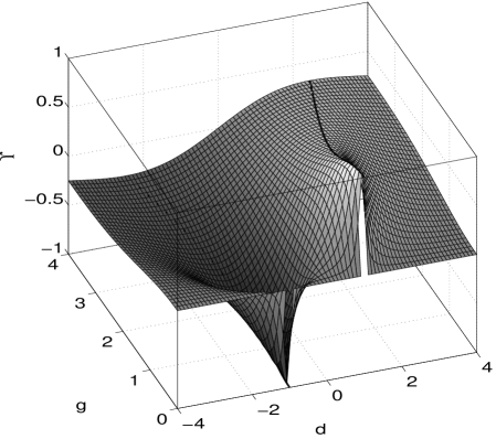
Figure 1: The function $\Upsilon\left(d,g\right)$.

IV Integrated Spectral Density

In general consider an operator $c\left(\omega\right)$ that can be expressed in terms of a noise operator $F\left(\omega\right)$ and a susceptibility matrix $\chi\left(\omega\right)$ as [similarly to Eqs. (LABEL:c_a(omega)) and (LABEL:c_b(omega))]

$$\left(\begin{array}[c]{c}c\left(\omega\right)\\ c^{{\dagger}}\left(-\omega\right)\end{array}\right)=\chi\left(\omega\right)\left(\begin{array}[c]{c}F\left(\omega\right)\\ F^{{\dagger}}\left(-\omega\right)\end{array}\right)\;,$$ (150)

where $F\left(\omega\right)$ satisfy [similarly to Eqs. (61), (62), (63), (64), (65) and (66)]

$$\left\langle F\left(\omega\right)\right\rangle=\left\langle F^{\dagger}\left(\omega\right)\right\rangle=0\ ,$$ (151)

$$\left\langle F\left(\omega\right)F\left(\omega^{\prime}\right)\right\rangle=\left\langle F^{\dagger}\left(\omega\right)F^{\dagger}\left(\omega^{\prime}\right)\right\rangle=0\ ,$$ (152)

$$\left\langle F\left(\omega\right)F^{\dagger}\left(\omega^{\prime}\right)\right\rangle=2\Gamma\delta\left(\omega-\omega^{\prime}\right)n_{\omega_{0}}\ ,$$ (153)

and

$$\left\langle F^{\dagger}\left(\omega\right)F\left(\omega^{\prime}\right)\right\rangle=2\Gamma\delta\left(\omega-\omega^{\prime}\right)\left(n_{\omega_{0}}+1\right)\ .$$ (154)

The homodyne detection observable $X\left(\omega\right)$ is defined by

$$X\left(\omega\right)=e^{i\phi_{\mathrm{LO}}}c\left(\omega\right)+e^{-i\phi_{\mathrm{LO}}}c^{{\dagger}}\left(-\omega\right)\ .$$ (155)

The frequency auto-correlation function of $X$ is related to the spectral density $P_{X}\left(\omega\right)$ by

$$\left\langle X^{{\dagger}}\left(\omega^{\prime}\right)X\left(\omega\right)\right\rangle=P_{X}\left(\omega\right)\delta\left(\omega-\omega^{\prime}\right)\ .$$ (156)

Assuming that $\chi\left(\omega\right)$ is omega-symmetric, it can be expressed as

$$\chi\left(\omega\right)=\left(\begin{array}[c]{cc}a\left(\omega\right)&b\left(\omega\right)\\ b^{\ast}\left(-\omega\right)&a^{\ast}\left(-\omega\right)\end{array}\right)\;,$$ (157)

where $a\left(\omega\right)$ and $b\left(\omega\right)$ are arbitrary functions of $\omega$. Thus, by calculating the term $\left\langle X^{{\dagger}}\left(\omega^{\prime}\right)X\left(\omega\right)\right\rangle$ one finds that

$$\frac{P_{X}\left(\omega\right)}{2\Gamma} =M_{+}\left(\omega\right)\coth\frac{\beta\hbar\omega_{0}}{2}+M_{-}\left(\omega\right)\ .$$

(158)

where

$$M_{+}\left(\omega\right) =\frac{\left|a\left(-\omega\right)\right|^{2}+\left|b\left(\omega\right)\right|^{2}+\left|a\left(\omega\right)\right|^{2}+\left|b\left(-\omega\right)\right|^{2}}{2}$$

$$+\operatorname{Re}\left[e^{2i\phi_{\mathrm{LO}}}\left(a\left(-\omega\right)b\left(\omega\right)+a\left(\omega\right)b\left(-\omega\right)\right)\right]\;,$$

(159)

and

$$M_{-}\left(\omega\right) =\frac{-\left|a\left(-\omega\right)\right|^{2}-\left|b\left(\omega\right)\right|^{2}+\left|a\left(\omega\right)\right|^{2}+\left|b\left(-\omega\right)\right|^{2}}{2}$$

$$+\operatorname{Re}\left[e^{2i\phi_{\mathrm{LO}}}\left(-a\left(-\omega\right)b\left(\omega\right)+a\left(\omega\right)b\left(-\omega\right)\right)\right]\;.$$

(160)

The integrated spectral density (ISD) is thus given by

$$\int\limits_{-\infty}^{\infty}\mathrm{d}\omega\;P_{X}\left(\omega\right)=2\Gamma V\coth\frac{\beta\hbar\omega_{0}}{2}\ ,$$ (161)

where

$$V =\int\limits_{-\infty}^{\infty}\mathrm{d}\omega\;M_{+}\left(\omega\right)$$

$$=\int\limits_{-\infty}^{\infty}\mathrm{d}\omega\;\left[\left|a\left(\omega\right)\right|^{2}+\left|b\left(-\omega\right)\right|^{2}+2\operatorname{Re}\left(e^{2i\phi_{\mathrm{LO}}}a\left(\omega\right)b\left(-\omega\right)\right)\right]\ .$$

(162)

V ISD of $X_{b}$

We calculate below the ISD of the homodyne observable $X_{b}\left(\omega\right)$, which is given by

$$X_{b}\left(\omega\right)=e^{i\phi_{\mathrm{LO}}}c_{b}\left(\omega\right)+e^{-i\phi_{\mathrm{LO}}}c_{b}^{{\dagger}}\left(-\omega\right)\ ,$$ (163)

for the case where $\Omega$ is small and $K_{a}=\gamma_{a3}=0$. As can be seen from Eq. (LABEL:c_b(omega)), it has two contributions due to the two uncorrelated noise terms $F_{b}\left(\omega\right)$ and $F_{a}\left(\omega\right)$. The calculation of both contributions according to Eq. (161) is involved with evaluation of some integrals, which can be performed using the residue theorem. To further simplify the final result, which is given by

$$\frac{1}{2\pi}\int\limits_{-\infty}^{\infty}\mathrm{d}\omega\;P_{X_{b}}\left(\omega\right)$$

$$=\left(1-\frac{\Omega^{2}E_{a}}{\gamma_{a}\gamma_{b}}\Upsilon\left(d,g\right)\right)\coth\frac{\beta\hbar\omega_{b}}{2}$$

$$+\frac{\Omega^{2}E_{a}}{\gamma_{a}\gamma_{b}}\frac{2g^{2}}{\left(1-d\right)^{2}+g^{2}}\coth\frac{\beta\hbar\omega_{a}}{2}\ ,$$

the case where resonator $b$ has high quality factor is assume. For this case, which is experimentally common, the following is assumed to hold $\gamma_{b}\ll\omega_{b}$ and $\gamma_{b}\ll\gamma_{a}$. As can be seen from Eq. (LABEL:ISD_gb_ss_ga), for finite driven amplitude $E_{a}$ the ISD of $X_{b}$ can deviate from the equilibrium value of $\coth\left(\beta\hbar\omega_{b}/2\right)$.

VI Decoherence

The Hamiltonian of the system (2) is formally a function of $A_{b}$ and $A_{b}^{\dagger}$, that is $\mathcal{H}=\mathcal{H}\left(A_{b},A_{b}^{{\dagger}}\right)$. Consider resonator $b$ in a superposition of two coherent states $\left|\alpha_{1}\right\rangle$ and $\left|\alpha_{2}\right\rangle$. In therm of the operator $\mathcal{V}$, which is given by

$$\mathcal{V}=\mathcal{H}\left(\alpha_{2},\alpha_{2}^{\ast}\right)-\mathcal{H}\left(\alpha_{1},\alpha_{1}^{\ast}\right)\;,$$ (165)

the decoherence rate $1/\tau_{\varphi}$ can be expressed as Levinson_299

$$\frac{1}{\tau_{\varphi}}=\frac{1}{\hbar^{2}}\int_{-\infty}^{\infty}\mathrm{d}\omega\;\left\langle\mathcal{\tilde{V}}\left(0\right)\mathcal{\tilde{V}}\left(\omega\right)\right\rangle\;,$$ (166)

where

$$\mathcal{\tilde{V}}\left(t\right)=\mathcal{V}\left(t\right)-\left\langle\mathcal{V}\left(t\right)\right\rangle\;,$$ (167)

and where $\mathcal{\tilde{V}}\left(\omega\right)$ is the Fourier transform of $\mathcal{\tilde{V}}\left(t\right)$

$$\mathcal{\tilde{V}}\left(t\right)=\frac{1}{\sqrt{2\pi}}\int_{-\infty}^{\infty}\mathrm{d}\omega\;\mathcal{\tilde{V}}\left(\omega\right)e^{-i\omega t}\;.$$ (168)

Using Eqs. (35) and (LABEL:c_a(omega)) together with the notation

$$\delta_{\alpha}=\alpha_{2}-\alpha_{1}=\left|\delta_{\alpha}\right|e^{i\theta}\;,$$ (169)

one finds to lowest order that

$$\frac{\mathcal{\tilde{V}}\left(\omega\right)}{\hbar\left|\delta_{\alpha}\right|}=U_{a}F_{a}\left(\omega\right)+U_{a}^{\ast}F_{a}^{{\dagger}}\left(-\omega\right)+U_{b}F_{b}\left(\omega\right)+U_{b}^{\ast}F_{b}^{{\dagger}}\left(-\omega\right)\;,$$ (170)

where

$$U_{a} =2\Omega\cos\theta\left(B_{a}^{\ast}\left(\chi_{aa}\right)_{11}+B_{a}\left(\chi_{aa}\right)_{21}\right)\;,$$ (171a)

$$U_{b} =2\Omega\cos\theta\left(B_{a}^{\ast}\left(\chi_{ab}\right)_{11}+B_{a}\left(\chi_{ab}\right)_{21}\right)+ie^{-i\theta}\;.$$ (171b)

Furthermore, with the help of Eqs. (63), (64), (65) and (66) the decoherence rate becomes

$$\frac{1}{\tau_{\varphi}} =2\left|\delta_{\alpha}\right|^{2}\left(\Gamma_{a}\left|U_{a}\right|^{2}\coth\frac{\beta\hbar\omega_{a}}{2}+\gamma_{b}\left|U_{b}\right|^{2}\coth\frac{\beta\hbar\omega_{b}}{2}\right)\;.$$

(172)

Note that for $\Omega=0$ the decoherence rate reproduces the value given by Eq. (1).

For the case where $\Omega$ is small and $K_{a}=\gamma_{a3}=0$ one finds using Eqs. (131) and (132) that

$$\left|U_{a}\right|^{2}=\frac{4\Omega^{2}E_{a}\cos^{2}\theta}{\omega_{b}^{2}\left(d^{2}+g^{2}\right)}\;,$$ (173)

and

$$\left|U_{b}\right|^{2}=1+\frac{4\Omega^{2}E_{a}\left[\cos a+\cos\left(2\theta+a\right)\right]}{\omega_{b}^{2}\sqrt{1+\left(\frac{\gamma_{b}}{\omega_{b}}\right)^{2}}}\frac{d}{d^{2}+g^{2}}\;.$$ (174)

where

$$a=\tan^{-1}\frac{\gamma_{b}}{\omega_{b}}\;.$$ (175)

In what follows we restrict the discussion to the case where $\theta=0$, for which the two coherent states $\left|\alpha_{1}\right\rangle$ and $\left|\alpha_{2}\right\rangle$ have the same momentum. For this case, which is the assumed case in some of the published proposals for observation of quantum superposition in mechanical systems Bose_4175 ; Bose_3204 ; Buks_174504 , up to first order in $\gamma_{b}/\omega_{b}$ one has

$$\left|U_{b}\right|^{2}=1+\frac{4\Omega^{2}E_{a}}{\omega_{b}^{2}}\frac{d}{d^{2}+g^{2}}\;.$$ (176)

Using these results together with Eq. (172) one finds that

$$\frac{1}{\tau_{\varphi}} =2\gamma_{b}\left|\delta_{\alpha}\right|^{2}$$

$$\times\left[\left(1+\frac{4\Omega^{2}E_{a}}{\omega_{b}^{2}}\frac{d}{d^{2}+g^{2}}\right)\coth\frac{\beta\hbar\omega_{b}}{2}\right.$$

$$+\left.\frac{\gamma_{a}}{\gamma_{b}}\frac{4\Omega^{2}E_{a}}{\omega_{b}^{2}}\frac{1}{d^{2}+g^{2}}\coth\frac{\beta\hbar\omega_{a}}{2}\right]\;.$$

(177)

The first term in Eq. (177) represents the contribution of the thermal bath that is directly coupled to resonator $b$ to the dephasing rate. This contribution can be either enhanced ($d>0$) or suppressed ($d<0$) due to back-reaction effects. On the other hand, the last term in Eq. (177) [compare with Eq. (71) of Ref. Buks_023815 ] represents the direct contribution of the driven resonator $a$. This contribution can be understood in terms of the shift in the effective resonance frequency of resonator $a$ between the two values corresponding to the two coherent states $\left|\alpha_{1}\right\rangle$ and $\left|\alpha_{2}\right\rangle$ (see Ref. Buks_023815 ).

VII Discussion

We have considered above the case where $\Omega$ is small, $K_{a}=\gamma_{a3}=0$ and $\gamma_{b}\ll\omega_{b}$. In addition, we have assumed that $\gamma_{a}\ll\gamma_{b}$ in order to obtain the ISD of $X_{b}$, which is given by Eq. (LABEL:ISD_gb_ss_ga), and we have assumed the case $\theta=0$ to obtain the dephasing rate, which is given by Eq. (177). Furthermore, consider for simplicity the case of high temperature where $\beta\hbar\omega_{b}\ll 1$. For this case Eqs. (LABEL:ISD_gb_ss_ga) and (177) can be written in terms of the effective temperatures $T_{\mathrm{ISD}}$ and $T_{\mathrm{D}}$

$$\frac{1}{2\pi}\int\limits_{-\infty}^{\infty}\mathrm{d}\omega\;P_{X_{b}}\left(\omega\right)=\frac{2k_{\mathrm{B}}T_{\mathrm{ISD}}}{\hbar\omega_{b}}\ ,$$ (178)

$$\frac{1}{\tau_{\varphi}}=2\gamma_{b}\left|\delta_{\alpha}\right|^{2}\frac{2k_{\mathrm{B}}T_{\mathrm{D}}}{\hbar\omega_{b}}\;,$$ (179)

where

$$\frac{T_{\mathrm{ISD}}}{T}=1-\frac{\Omega^{2}E_{a}\Upsilon\left(d,g\right)}{\gamma_{a}\gamma_{b}}\left(1-\frac{\omega_{b}\Theta_{a}}{\omega_{a}}\frac{\left(1+d\right)^{2}+g^{2}}{3d}\right)\;,$$ (180)

$$\frac{T_{\mathrm{D}}}{T}=1+\frac{4\Omega^{2}E_{a}}{\omega_{b}^{2}}\frac{d}{d^{2}+g^{2}}\left(1+\frac{\omega_{b}\gamma_{a}\Theta_{a}}{\omega_{a}\gamma_{b}}\frac{1}{d}\right)\;,$$ (181)

and

$$\Theta_{a}=\frac{\beta\hbar\omega_{a}}{2}\coth\frac{\beta\hbar\omega_{a}}{2}\;.$$ (182)

In terms of $\left(E_{a}\right)_{c}$, which is given by Eq. (146), one thus has

$$\frac{T_{\mathrm{ISD}}}{T}=1-\frac{E_{a}}{\left(E_{a}\right)_{c}}\frac{\omega_{b}\Upsilon\left(d,g\right)}{\sqrt{3}\gamma_{b}}\left(1-\frac{\omega_{b}\Theta_{a}}{\omega_{a}}\frac{\left(1+d\right)^{2}+g^{2}}{3d}\right)\;,$$ (183)

and

$$\frac{T_{\mathrm{D}}}{T}=1+\frac{4E_{a}}{\sqrt{3}\left(E_{a}\right)_{c}}\frac{dg}{d^{2}+g^{2}}\left(1+\frac{\omega_{b}\gamma_{a}\Theta_{a}}{\omega_{a}\gamma_{b}}\frac{1}{d}\right)\;.$$ (184)

These results are valid only to lowest order in $\Omega$, however they may be used in some cases to roughly estimate the lowest possible values of $T_{\mathrm{ISD}}$ and $T_{\mathrm{D}}$. As can be seen from Eqs. (183) and (184), the effective temperatures $T_{\mathrm{ISD}}$ and $T_{\mathrm{D}}$ may take considerably different values. This fact should not be considered as surprising since the system is far from thermal equilibrium and since the underlying mechanisms responsible for ISD reduction and for suppression of decoherence are entirely different. In what follows, we choose the parameters $d$ and $g$ such that the largest reduction in effective temperature is achieved for a given $E_{a}$, and use these values to estimate the lowest possible effective temperatures.

VII.1 Optimum ISD Reduction

For the case of ISD reduction, we consider the case where the term that is proportional to $\Theta_{a}$ in Eq. (183), namely the term which represents the contribution of the thermal baths that are directly coupled to resonator $a$, is relatively small, namely the case where $\omega_{b}\Theta_{a}\ll\omega_{a}$. This condition is expected to be fulfilled for the typical experimental situation. Most efficient ISD reduction is achieved by choosing the parameters $g\ll 1$ and $d=1$, for which the term $\Upsilon\left(d,g\right)$ obtains its maximum possible value $\Upsilon=1$ (see Fig. 1). For this case Eq. (183) becomes

$$\frac{T_{\mathrm{ISD}}}{T}=1-\frac{\omega_{b}}{\sqrt{3}\gamma_{b}}\frac{E_{a}}{\left(E_{a}\right)_{c}}\left(1-\frac{4\omega_{b}\Theta_{a}}{3\omega_{a}}\right)\;.$$ (185)

By taking

$$E_{a}=\frac{\sqrt{3}\gamma_{b}}{\omega_{b}}\left(E_{a}\right)_{c}\equiv\left(E_{a}\right)_{\mathrm{ISD}}\;,$$ (186)

Eq. (185) yields the lowest possible value of $T_{\mathrm{ISD}}$, which is denoted as $\left(T_{\mathrm{ISD}}\right)_{\min}$

$$\frac{\left(T_{\mathrm{ISD}}\right)_{\min}}{T}=\frac{4\omega_{b}\Theta_{a}}{3\omega_{a}}\;.$$ (187)

As was mentioned above, the above discussion is based on the approximated result Eq. (183), which expresses $T_{\mathrm{ISD}}$ to lowest nonvanishing order in $\Omega$. Such an expansion apparently suggests that the noise contribution due to the thermal bath that is directly coupled to resonator $b$ can be altogether eliminated, leaving thus only the noise contribution of the thermal baths that are directly coupled to resonator $a$ as a lower bound imposed upon $T_{\mathrm{ISD}}$ [see Eq. (187)]. Obviously, however, higher orders in $\Omega$ have to be taken into account in order estimate $\left(T_{\mathrm{ISD}}\right)_{\min}$ more accurately, as was done in Ref. Blencowe_014511 , where $T_{\mathrm{ISD}}$ was expanded up to forth order in $\Omega$.

VII.2 Decoherence Suppression

For the case of decoherence suppression, on the other hand, the term that is proportional to $\Theta_{a}$ in Eq. (184) is not necessarily small for the common experimental situation. We therefore chose the optimum values of the parameters $d$ and $g$ for the more general case. Using the notation

$$D=\frac{\omega_{b}\gamma_{a}\Theta_{a}}{\omega_{a}\gamma_{b}}\;,$$ (188)

Eq. (184) reads

$$\frac{T_{\mathrm{D}}}{T}=1+\frac{4E_{a}}{\sqrt{3}\left(E_{a}\right)_{c}}f\left(d,g,D\right)\;.$$ (189)

where

$$f\left(d,g,D\right)=\frac{dg}{d^{2}+g^{2}}\left(1+\frac{D}{d}\right)\;.$$ (190)

In general, the minimum value of the function $f\left(d,g,D\right)$ for a given $g>0$ and a given $D>0$ is obtained at

$$d_{\mathrm{m}}=-D-\sqrt{D^{2}+g^{2}}\;,$$ (191)

and the minimum value is given by

$$f\left(d_{\mathrm{m}},g,D\right)=-\frac{1}{2}\tan\left(\frac{\tan^{-1}\frac{g}{D}}{2}\right)\;.$$ (192)

The lowest value of $f\left(d_{\mathrm{m}},g,D\right)$ is thus obtained in the limit $D\ll g$, for which one finds that $d_{\mathrm{m}}=-g$ and $f\left(d_{\mathrm{m}},g,D\right)=-1/2$. Therefore, one concludes that the largest reduction in $T_{\mathrm{D}}$ for a given $E_{a}$ is obtained when

$$\frac{\omega_{b}^{2}\Theta_{a}}{\omega_{a}\gamma_{b}}\ll 1\;$$ (193)

and when $d=-g$. For this case Eq. (184) becomes

$$\frac{T_{\mathrm{D}}}{T}=1-\frac{2}{\sqrt{3}}\frac{E_{a}}{\left(E_{a}\right)_{c}}\;.$$ (194)

This results indicates that even when all parameters are optimally chosen such that the largest reduction in $T_{\mathrm{D}}$ is obtained for a given $E_{a}$, no significant reduction in $T_{\mathrm{D}}$ is possible unless $E_{a}$ becomes comparable with $\left(E_{a}\right)_{c}$. Note, however, that in our analysis of the present case the effect of nonlinear bistability has been disregarded. This approximation can be justified for the case of ISD reduction since, as can be seen from Eq. (186), optimum reduction of the ISD can be achieved well below the bistability threshold provided that $\gamma_{b}\ll\omega_{b}$. On the other hand, Eq. (194) indicates that optimum suppression of decoherence can be achieved only very close to the bistability threshold. In this region, however, our approximated treatment breaks down and Eq. (184) becomes inaccurate.

To calculate $T_{\mathrm{D}}$ near the bistability threshold we thus numerically evaluate the dephasing rate given by Eq. (172) without assuming that $\Omega$ is small or $K_{a}=\gamma_{a3}=0$. As before, we take $\theta=0$ and consider for simplicity the case where $\beta\hbar\omega_{b}\ll 1$, for which the effective temperature $T_{\mathrm{D}}$ is given by

$$\frac{T_{\mathrm{D}}}{T}=\left|U_{b}\right|^{2}+\frac{\Gamma_{a}\omega_{b}\left|U_{a}\right|^{2}}{\omega_{a}\gamma_{b}}\Theta_{a}\;.$$ (195)

Figure 2 shows an example calculation of the parameters $\left|U_{b}\right|^{2}$ and $\left|U_{a}\right|^{2}$ and the ratio $T_{\mathrm{D}}/T$ near bistability threshold of the system. The ratio $T_{\mathrm{D}}/T$ is shown for the case where $\beta\hbar\omega_{a}\ll 1$. The set of system’s parameters chosen for this example is listed in the caption of Fig. 2. The stability of the mean filed solution is checked by evaluating the eigenvalues of the matrix $W$. The dotted sections of the curve $T_{\mathrm{D}}/T$ indicate the regions in which the solution is unstable (where at least one of the eigenvalues of $W$ has a negative real part). Near the onset of bistability point [see panel (c4) of Fig. 2] and near jump points in the region of bistability [see panel (d4) of Fig. 2] the ratio $T_{\mathrm{D}}/T$ may become relatively small. This behavior can be attributed to critical slowing down, which occurs near these instability points Buks_023815 . On the other hand, in the vicinity of these points the solution becomes unstable [see the dotted sections of the curve $T_{\mathrm{D}}/T$ in panels (c4) and (d4) of Fig. 2]. When the unstable region is excluded one finds that no significant reduction in the ratio $T_{\mathrm{D}}/T$ can be achieved for this particular example (the lowest value is about $0.5$).

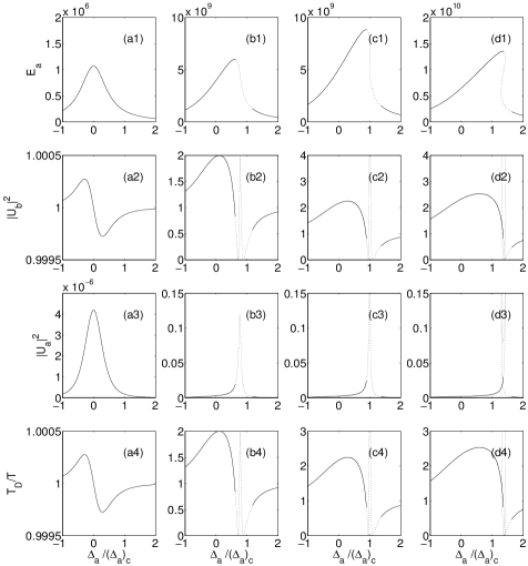
Figure 2: The factors $\left|U_{b}\right|^{2}$ and $\left|U_{a}\right|^{2}$ and the ratio $T_{\mathrm{D}}/T$. The driving amplitudes in columns a, b, c and d are $b_{p}/\left(b_{p}\right)_{c}=0.01$, $0.8$, $1$ and $1.3$ respectively. Other system parameters are $\Omega/\omega_{a}=10^{-10}$, $\omega_{b}/\omega_{a}=10^{-6}$, $\gamma_{b}/\omega_{b}=10^{-3}$, $K_{a}=2\times 2\Omega^{2}\omega_{b}/\left(\omega_{b}^{2}+\gamma_{b}^{2}\right)$, $\theta=0$, $\gamma_{a1}/\omega_{b}=10^{2}$, $\gamma_{a2}/\gamma_{a1}=10^{-2}$ and $\gamma_{a3}=0.1\times\left|K_{a}^{\mathrm{eff}}\right|/\sqrt{3}$. The ratio $T_{\mathrm{D}}/T$, which is plotted in the forth row, is shown for the case $\beta\hbar\omega_{a}\ll 1$. The dotted sections indicate instability.

In the previous example the mean-field solutions become unstable close to the onset of bistability. This behavior prevents any significant suppression of decoherence, namely, the ratio $T_{\mathrm{D}}/T$ could not be made much smaller than unity. To overcome this limitation the parameter $\left(E_{a}\right)_{c}$, which is given by Eq. (53), has to be increased without, however, increasing the coupling parameter $\Omega$. We point out below two possibilities to achieve this. In the first one, the parameter $K_{a}$ is chosen such that $K_{a}\simeq 2\Omega^{2}\omega_{b}/\left(\omega_{b}^{2}+\gamma_{b}^{2}\right),$ and consequently $K_{a}^{\mathrm{eff}}$ becomes very small [see Eq. (45)]. In the second one, which is demonstrated in Fig. 3 below, the nonlinear damping rate $\gamma_{a3}$ is chosen very close to the largest possible value of $\left|K_{a}^{\mathrm{eff}}\right|/\sqrt{3}$ for which bistability is accessible [see inequality (50)]. As can be see from Eq. (53), both possibilities allow significantly increasing the parameter $\left(E_{a}\right)_{c}$. For the example shown in Fig. 3 below, the value $\gamma_{a3}=0.99\left|K_{a}^{\mathrm{eff}}\right|/\sqrt{3}$ is chosen and all other parameters are the same as in the previous example (see caption of Fig. 2). As can be seen from panels (c4) and (d4) of Fig. 3, much lower values of the ratio $T_{\mathrm{D}}/T$ are achievable in the present example (a lowest value of about $0.02$ is obtained at the edge of the region where the solution is stable). This improvement can be attributed to the stabilization effect of the nonlinear damping. It is important to point out, however, that implementation of any of the two above mentioned possibilities require that the nonlinear parameters of resonator $a$ ($K_{a}$ and/or $\gamma_{a3}$) can be accurately tuned to the desired values. Such tuning of nonlinear parameters can possibly becomes achievable by exploiting effects arising from thermo-optomechanical coupling Zaitsev_1104_2237 .

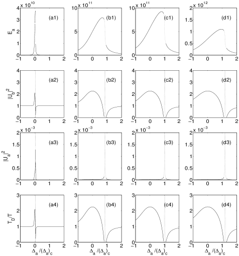
Figure 3: The factors $\left|U_{b}\right|^{2}$ and $\left|U_{a}\right|^{2}$ and the ratio $T_{\mathrm{D}}/T$. In this example $\gamma_{a3}=0.99\times\left|K_{a}^{\mathrm{eff}}\right|/\sqrt{3}$ whereas all other parameters are the same as in the previous example [see caption of Fig. (2)].

References

- (1) Miles Blencowe, “Quantum electromechanical systems,” Phys. Rep., vol. 395, pp. 159–222, 2004.
- (2) Keith C. Schwab and Michael L. Roukes, “Putting mechanics into quantum mechanics,” Phys. Today, vol. July, pp. 36–42, 2005.
- (3) A. D. O Connell, M. Hofheinz, M. Ansmann, Radoslaw C. Bialczak, M. Lenander, Erik Luceroand M. Neeley, D. Sank, H. Wang, M. Weides, J. Wenner, John M. Martinis, and A. N. Cleland, “Quantum ground state and single-phonon control of a mechanical resonator,” Nature, vol. 464, pp. 697–703, 2010.
- (4) A. J. Leggett, “Testing the limits of quantum mechanics: Motivation, state of play, prospects,” J. Phys. Condens. Matter, vol. 14, pp. R415, 2002.
- (5) A. J. Leggett and Anupam Garg, “Quantum mechanics versus macroscopic realism: Is the flux there when nobody looks?,” Phys. Rev. Lett., vol. 54, pp. 857–860, 1985.
- (6) Roger Penrose, “On gravity’s role in quantum state reduction,” Gen. Relativ. Gravit., vol. 28, pp. 581–600, 1996.
- (7) L. Diosi, “Models for universal reduction of macroscopic quantum fluctuations,” Phys. Rev. A, vol. 40, pp. 1165–1174, 1989.
- (8) S. Bose, K. Jacobs, and P. L. Knight, “Preparation of nonclassical states in cavities with a moving mirror,” Phys. Rev. A, vol. 56, pp. 4175, 1997.
- (9) S. Bose, K. Jacobs, and P. L. Knight, “Scheme to probe the decoherence of a macroscopic object,” Phys. Rev. A, vol. 59, pp. 3204–3210, 1999.
- (10) Dustin Kleckner, Igor Pikovski, Evan Jeffrey, Luuk Ament, Eric Eliel, Jeroen Van Den Brink, and Dirk Bouwmeester, “Creating and verifying a quantum superposition in a micro-optomechanical system,” New J. Phys., vol. 10, pp. 095020, 2008.
- (11) Wojciech H. Zurek, “Decoherence and the transition from quantum to classical – REVISITED,” arXiv:quant-ph/0306072, 2003.
- (12) Wojciech Hubert Zurek, “Decoherence, einselection, and the quantum origins of the classical,” Rev. Mod. Phys., vol. 75, pp. 715–775, 2003.
- (13) A. O. Caldeira and A. J. Leggett, “Path integral approach to quantum brownian motion,” Physica A, vol. 121, pp. 587, 1983.
- (14) E. Joos and H. D. Zeh, “The emergence of classical properties through interaction with the environment,” Physik B, vol. 59, pp. 223, 1985.
- (15) W. G. Unruh and W. H. Zurek, “Reduction of a wave packet in quantum brownian motion,” Phys. Rev. D, vol. 40, pp. 1071, 1989.
- (16) W. H. Zurek, “Decoherence and the transition from quantum to classical,” Physics Today, vol. 44, pp. 36, 1991.
- (17) D. Rugar and P. Grutter, “Mechanical parametric amplification and thermomechanical noise squeezing,” Phys. Rev. Lett., vol. 67, pp. 699, 1991.
- (18) R. Almog, S. Zaitsev, O. Shtempluck, and E. Buks, “Noise squeezing in a nanomechanical duffing resonator,” Phys. Rev. Lett., vol. 98, pp. 78103, 2007.
- (19) H. J. Kimble, Y. Levin, A. B. Matsko, K. S. Thorne, and S. P. Vyatchanin, “Conversion of conventional gravitational-wave interferometers into quantum nondemolition interferometers by modifying their input and/or output optics,” Phys. Rev. D, vol. 65, pp. 022002, Dec 2001.
- (20) V. B. Braginsky and S. P. Vyatchanin, “Low quantum noise tranquilizer for Fabry Perot interferometer,” Phys. Lett. A, vol. 293, pp. 228–234, 2002.
- (21) Ivar Martin, Alexander Shnirman, Lin Tian, and Peter Zoller, “Ground-state cooling of mechanical resonators,” Phys. Rev. B, vol. 69, pp. 125339, 2004.
- (22) I. Wilson-Rae, P. Zoller, and A. Imamolu, “Laser cooling of a nanomechanical resonator mode to its quantum ground state,” Phys. Rev. Lett., vol. 92, pp. 75507, 2004.
- (23) Aashish A Clerk and Steven Bennett, “Quantum nanoelectromechanics with electrons, quasi-particles and cooper pairs: Effective bath descriptions and strong feedback effects,” New J. Phys., vol. 7, pp. 238, 2005.
- (24) M. P. Blencowe, J. Imbers, and A. D. Armour, “Dynamics of a nanomechanical resonator coupled to a superconducting single-electron transistor,” New J. Phys., vol. 7, pp. 236, 2005.
- (25) D. J. Wineland, J. Britton, R. J. Epstein, D. Leibfried, R. B. Blakestad, K. Brown, J. D. Jost, C. Langer, R. Ozeri, S. Seidelin, and J. Wesenberg, “Cantilever cooling with radio frequency circuits,” arXiv: quant-ph/0606180, 2006.
- (26) Florian Marquardt, Joe P. Chen, A. A. Clerk, and S. M. Girvin, “Quantum theory of cavity-assisted sideband cooling of mechanical motion,” Phys. Rev. Lett., vol. 99, pp. 93902, 2007.
- (27) V. B. Braginsky and A. B. Manukin, “Ponderomotive effects of electromagnetic radiation (in Russian),” ZhETF, vol. 52, pp. 986–989, 1967.
- (28) V. B. Braginsky, A. B. Manukin, and M. Yu. Tikhonov, “Investigation of dissipative ponderomotive effects of electromagnetic radiation (in Russian),” ZhETF, vol. 58, pp. 1550–1555, 1970.
- (29) T. Corbitt, D. Ottaway, E. Innerhofer, J. Pelc, and N. Mavalvala, “Measurement of radiation-pressure-induced optomechanical dynamics in a suspended Fabry-Perot cavity,” Phys. Rev. A, vol. 74, pp. 021802, Aug 2006.
- (30) T. J. Kippenberg and K. J. Vahala, “Cavity optomechanics: Back-action at the mesoscale,” Science, vol. 321, no. 5893, pp. 1172–1176, Aug 2008.
- (31) A. Schliesser, R. Riviere, G. Anetsberger, O. Arcizet, and T. J. Kippenberg, “Resolved-sideband cooling of a micromechanical oscillator,” Nat. Phys., vol. 4, pp. 415–419, 2008.
- (32) C. Genes, D. Vitali, P. Tombesi, S. Gigan, and M. Aspelmeyer, “Ground-state cooling of a micromechanical oscillator: Comparing cold damping and cavity-assisted cooling schemes,” Phys. Rev. A, vol. 77, pp. 033804, Mar 2008.
- (33) J. D. Teufel, D. Li, M. S. Allman, K. Cicak, A. J. Sirois, J. D. Whittaker, and R. W. Simmonds, “Circuit cavity electromechanics in the strong coupling regime,” arXiv, Nov 2010.
- (34) S. Gigan, H. R. Böhm, M. Paternostro, F. Blaser, J. B. Hertzberg, K. C. Schwab, D. Bauerle, M. Aspelmeyer, and A.Zeilinger, “Self cooling of a micromirror by radiation pressure,” Nature, vol. 444, pp. 67–70, 2006.
- (35) O. Arcizet, P. F.Cohadon, T. Briant, M. Pinard, and A. Heidmann, “Radiation-pressure cooling and optomechanical instability of a micromirror,” Nature, vol. 444, pp. 71–74, 2006.
- (36) D. Kleckner and D. Bouwmeester, “Sub-kelvin optical cooling of a micromechanical resonator,” Nature, vol. 444, pp. 75–78, 2006.
- (37) T. Corbitt, Y. Chen, E. Innerhofer, H. Müller-Ebhardt, D. Ottaway, H. Rehbein, D. Sigg, S. Whitcomb, C. Wipf, and N. Mavalvala, “An all-optical trap for a gram-scale mirror,” Phys. Rev. Lett., vol. 98, pp. 150802, 2007.
- (38) A. Schliesser, P. Del Haye, N. Nooshi, K. J. Vahala, and T. J. Kippenberg, “Radiation pressure cooling of a micromechanical oscillator using dynamical backaction,” Phys. Rev. Lett., vol. 97, pp. 243905, 2006.
- (39) J. G. E. Harris, B. M. Zwickl, and A. M. Jayich, “Stable, mode-matched, medium-finesse optical cavity incorporating a microcantilever mirror: Optical characterization and laser cooling,” Rev. Sci. Instrum., vol. 78, pp. 13107, 2007.
- (40) A. Naik, O. Buu, M. D. LaHaye, A. D. Armour, A. A. Clerk, M. P. Blencowe, and K. C. Schwab, “Cooling a nanomechanical resonator with quantum back-action,” Nature, vol. 443, pp. 193–196, 2006.
- (41) Constanze Höhberger Metzger and Khaled Karrai, “Cavity cooling of a microlever,” Nature, vol. 432, pp. 1002–1005, 2004.
- (42) J. D. Teufel, T. Donner, Dale Li, J. H. Harlow, M. S. Allman, K. Cicak, A. J. Sirois, J. D. Whittaker, K. W. Lehnert, and R. W. Simmonds, “Sideband cooling micromechanical motion to the quantum ground state,” arXiv:1103.2144, 2011.
- (43) Bernard Yurke and Eyal Buks, “Performance of cavity-parametric amplifiers, employing kerr nonlinearites, in the presence of two-photon loss,” J. Lightwave Tech., vol. 24, pp. 5054–5066, 2006.
- (44) C. W. Gardiner and M. J. Collett, “Input and output in damped quantum systems: Quantum stochastic differential equations and the master equation,” Phys. Rev. A, vol. 31, pp. 3761, 1985.
- (45) Y. Levinson, “Dephasing in a quantum dot due to coupling with a quantum point contact,” Europhys. Lett., vol. 39, pp. 299–304, 1997.
- (46) Eyal Buks and M. P. Blencowe, “Decoherence and recoherence in a vibrating RF SQUID,” Phys. Rev. B, vol. 74, pp. 174504, 2006.
- (47) Eyal Buks and Bernard Yurke, “Dephasing due to intermode coupling in superconducting stripline resonators,” Phys. Rev. A, vol. 73, pp. 23815, 2006.
- (48) M. P. Blencowe and E. Buks, “Quantum analysis of a linear DC SQUID mechanical displacement detector,” Phys. Rev. B, vol. 76, pp. 14511, 2007.
- (49) Stav Zaitsev, Ashok K. Pandey, Oleg Shtempluck, and Eyal Buks, “Forced and self oscillations of optomechanical cavity,” arXiv:1104.2237, 2011.