1jdgier@unimelb.edu.au, 2c.finn3@pgrad.unimelb.edu.au, 3msorrell@unimelb.edu.au

Relaxation rate of the reverse biased asymmetric exclusion process

1Jan de Gier, 2Caley Finn and 3Mark Sorrell Department of Mathematics and Statistics, The University of Melbourne, 3010 VIC, Australia
Abstract

We compute the exact relaxation rate of the partially asymmetric exclusion process with open boundaries, with boundary rates opposing the preferred direction of flow in the bulk. This reverse bias introduces a length scale in the system, at which we find a crossover between exponential and algebraic relaxation on the coexistence line. Our results follow from a careful analysis of the Bethe ansatz root structure.

1 Introduction

The partially asymmetric exclusion process (PASEP) [1, 2] is one of the most thoroughly studied models of non-equilibrium statistical mechanics [3, 4, 5, 6]. It is a microscopic model of a driven system [7] describing the asymmetric diffusion of hard-core particles along a one-dimensional chain. In this paper we will consider a finite chain with L๐ฟL sites. At late times the PASEP exhibits a relaxation towards a non-equilibrium stationary state. In the presence of two boundaries at which particles are injected and extracted with given rates, the bulk behaviour at stationarity is strongly dependent on the injection and extraction rates. The corresponding stationary phase diagram as well as various physical quantities have been determined by exact methods [3, 4, 5, 8, 9, 10, 11, 12, 13, 6].

More recently exact dynamical properties such as relaxation rates have been derived. On an infinite lattice where random matrix techniques can be used, considerable progress has been made, see e.g. [14, 15, 16, 17]. For the PASEP on a finite ring, where particle number is conserved, relaxation rates were obtained by means of the Bethe ansatz some time ago [18, 19, 20, 21]. The dynamical phase diagram of the PASEP with open boundaries was studied in [22, 23, 24], again using Bethe ansatz methods.

In the present work we extend some of these results to the case of reverse bias, where the boundary parameters strongly oppose the bias in the bulk hopping rates. We will in particular focus on the coexistence line where the effects are most pronounced.

1.1 The partially asymmetric exclusion process

Refer to caption

Figure 1: Transition rates for the partially asymmetric exclusion process.

We now turn to a description of the dynamical rules defining the PASEP on a one dimensional lattice with L๐ฟL sites, see Figureย 1. At any given time t๐‘กt each site is either occupied by a particle or empty. The system is then updated as follows.

Particles attempt to hop one site to the right with rate p๐‘p and one site to the left with rate q๐‘žq. The hop is prohibited if the neighbouring site is occupied, and at sites 111 and L๐ฟL these rules are modified in the following way. If site i=1๐‘–1i=1 is empty, a particle may enter the system with rate ฮฑ๐›ผ\alpha. If, on the other hand, this site is occupied, the particle will leave the system with rate ฮณ๐›พ\gamma or attempt to hop to the right with rate p๐‘p. Similarly, at i=L๐‘–๐ฟi=L particles are injected and extracted with rates ฮด๐›ฟ\delta and ฮฒ๐›ฝ\beta respectively, and attempt to hop to the left with rate q๐‘žq.

It is customary to associate a Boolean variable ฯ„isubscript๐œ๐‘–\tau_{i} with every site, indicating whether a particle is present (ฯ„i=1subscript๐œ๐‘–1\tau_{i}=1) or not (ฯ„i=0subscript๐œ๐‘–0\tau_{i}=0) at site i๐‘–i. Let |0โŸฉket0|0\rangle and |1โŸฉket1|1\rangle denote the standard basis vectors in โ„‚2superscriptโ„‚2\mathbb{C}^{2}. A state of the system at time t๐‘กt is then characterised by the probability distribution

|Pโ€‹(t)โŸฉ=โˆ‘๐‰Pโ€‹(๐‰|t)โ€‹|๐‰โŸฉ,ket๐‘ƒ๐‘กsubscript๐‰๐‘ƒconditional๐‰๐‘กket๐‰|P(t)\rangle=\sum_{\bm{\tau}}P(\bm{\tau}|t)|\bm{\tau}\rangle, (1.1)

where

|๐‰โŸฉ=|ฯ„1,โ€ฆ,ฯ„LโŸฉ=โจ‚i=1L|ฯ„iโŸฉ.ket๐‰ketsubscript๐œ1โ€ฆsubscript๐œ๐ฟsuperscriptsubscripttensor-product๐‘–1๐ฟketsubscript๐œ๐‘–|\bm{\tau}\rangle=|\tau_{1},\ldots,\tau_{L}\rangle=\bigotimes_{i=1}^{L}|\tau_{i}\rangle. (1.2)

The time evolution of |Pโ€‹(t)โŸฉket๐‘ƒ๐‘ก|P(t)\rangle is governed by the aforementioned rules, which gives rise to the master equation

ddโ€‹tโ€‹|Pโ€‹(t)โŸฉdd๐‘กket๐‘ƒ๐‘ก\displaystyle\frac{{\rm d}}{{\rm d}t}|P(t)\rangle =\displaystyle= Mโ€‹|Pโ€‹(t)โŸฉ,๐‘€ket๐‘ƒ๐‘ก\displaystyle M|P(t)\rangle, (1.3)

where the PASEP transition matrix M๐‘€M consists of two-body interactions only and is given by

M=โˆ‘k=1Lโˆ’1I(kโˆ’1)โŠ—MkโŠ—I(Lโˆ’kโˆ’1)+m1โŠ—I(Lโˆ’1)+I(Lโˆ’1)โŠ—mL.๐‘€superscriptsubscript๐‘˜1๐ฟ1tensor-productsuperscript๐ผ๐‘˜1subscript๐‘€๐‘˜superscript๐ผ๐ฟ๐‘˜1tensor-productsubscript๐‘š1superscript๐ผ๐ฟ1tensor-productsuperscript๐ผ๐ฟ1subscript๐‘š๐ฟM=\sum_{k=1}^{L-1}I^{(k-1)}\otimes M_{k}\otimes I^{(L-k-1)}+m_{1}\otimes I^{(L-1)}+I^{(L-1)}\otimes m_{L}. (1.4)

Here I(k)superscript๐ผ๐‘˜I^{(k)} is the identity matrix on the k๐‘˜k-fold tensor product of โ„‚2superscriptโ„‚2\mathbb{C}^{2} and, for 1โ‰คkโ‰คLโˆ’11๐‘˜๐ฟ11\leq k\leq L-1, Mk:โ„‚2โŠ—โ„‚2โ†’โ„‚2โŠ—โ„‚2:subscript๐‘€๐‘˜โ†’tensor-productsuperscriptโ„‚2superscriptโ„‚2tensor-productsuperscriptโ„‚2superscriptโ„‚2M_{k}:\mathbb{C}^{2}\otimes\mathbb{C}^{2}\rightarrow\mathbb{C}^{2}\otimes\mathbb{C}^{2} is given by

Mk=(00000โˆ’qp00qโˆ’p00000).subscript๐‘€๐‘˜00000๐‘ž๐‘00๐‘ž๐‘00000\displaystyle M_{k}=\left(\begin{array}[]{@{}cccc@{}}0&0&0&0\\ 0&-q&p&0\\ 0&q&-p&0\\ 0&0&0&0\end{array}\right). (1.9)

The terms involving m1subscript๐‘š1m_{1} and mLsubscript๐‘š๐ฟm_{L} describe injection (extraction) of particles with rates ฮฑ๐›ผ\alpha and ฮด๐›ฟ\delta (ฮณ๐›พ\gamma and ฮฒ๐›ฝ\beta) at sites 111 and L๐ฟL respectively. Their explicit forms are

m1=(โˆ’ฮฑฮณฮฑโˆ’ฮณ),mL=(โˆ’ฮดฮฒฮดโˆ’ฮฒ).formulae-sequencesubscript๐‘š1๐›ผ๐›พ๐›ผ๐›พsubscript๐‘š๐ฟ๐›ฟ๐›ฝ๐›ฟ๐›ฝm_{1}=\left(\begin{array}[]{@{}cc@{}}-\alpha&\gamma\cr\alpha&-\gamma\cr\end{array}\right),\qquad m_{L}=\left(\begin{array}[]{@{}cc@{}}-\delta&\beta\cr\delta&-\beta\cr\end{array}\right). (1.10)

The transition matrix M๐‘€M has a unique stationary state corresponding to the eigenvalue zero. For positive rates, all other eigenvalues of M๐‘€M have non-positive real parts. The late time behaviour of the PASEP is dominated by the eigenstates of M๐‘€M with the largest real parts of the corresponding eigenvalues.

In the next sections we set p=1๐‘1p=1 without loss of generality and determine the eigenvalue of M๐‘€M with the largest non-zero real part using the Bethe ansatz. The latter reduces the problem of determining the spectrum of M๐‘€M to solving a system of coupled polynomial equations of degree 3โ€‹Lโˆ’13๐ฟ13L-1. Using these equations, the spectrum of M๐‘€M can be studied numerically for very large L๐ฟL, and, as we will show, analytic results can be obtained in the limit for large L๐ฟL.

1.2 Reverse bias

The reverse bias regime corresponds to the boundary parameters opposing the direction of flow in the bulk. In this paper we achieve this by considering the regime

q<1,ฮฑ,ฮฒโ‰ชฮณ,ฮด.formulae-sequence๐‘ž1๐›ผmuch-less-than๐›ฝ๐›พ๐›ฟq<1,\quad\alpha,\beta\ll\gamma,\delta. (1.11)

With q<1๐‘ž1q<1 the bias in the bulk is for diffusion left to right, but setting ฮฑ,ฮฒโ‰ชฮณ,ฮดformulae-sequencemuch-less-than๐›ผ๐›ฝ๐›พ๐›ฟ\alpha,\beta\ll\gamma,\delta strongly favours particles entering from the right and exiting on the left. Traditionally the reverse bias regime was considered only to exist for the case ฮฑ=ฮฒ=0๐›ผ๐›ฝ0\alpha=\beta=0, see e.g. [13]111Note that the authors of [13] consider q>1๐‘ž1q>1 and ฮณ=ฮด=0๐›พ๐›ฟ0\gamma=\delta=0 but we can simply translate their results to our notation using left-right symmetry.

2 Stationary phase diagram

In this section we briefly review some known facts about the stationary phase diagram. It will be convenient to use the following standard combinations of parameters [10],

ฮบฮฑ,ฮณยฑ=12โ€‹ฮฑโ€‹(vฮฑ,ฮณยฑvฮฑ,ฮณ2+4โ€‹ฮฑโ€‹ฮณ),vฮฑ,ฮณ=1โˆ’qโˆ’ฮฑ+ฮณ.formulae-sequencesubscriptsuperscript๐œ…plus-or-minus๐›ผ๐›พ12๐›ผplus-or-minussubscript๐‘ฃ๐›ผ๐›พsuperscriptsubscript๐‘ฃ๐›ผ๐›พ24๐›ผ๐›พsubscript๐‘ฃ๐›ผ๐›พ1๐‘ž๐›ผ๐›พ\kappa^{\pm}_{\alpha,\gamma}=\frac{1}{2\alpha}\left(v_{\alpha,\gamma}\pm\sqrt{v_{\alpha,\gamma}^{2}+4\alpha\gamma}\right),\qquad v_{\alpha,\gamma}=1-q-\alpha+\gamma. (2.1)

In order to ease notations we will use the following abbreviations,

a=ฮบฮฑ,ฮณ+,b=ฮบฮฒ,ฮด+,c=ฮบฮฑ,ฮณโˆ’,d=ฮบฮฒ,ฮดโˆ’.formulae-sequence๐‘Žsubscriptsuperscript๐œ…๐›ผ๐›พformulae-sequence๐‘subscriptsuperscript๐œ…๐›ฝ๐›ฟformulae-sequence๐‘subscriptsuperscript๐œ…๐›ผ๐›พ๐‘‘subscriptsuperscript๐œ…๐›ฝ๐›ฟa=\kappa^{+}_{\alpha,\gamma},\quad b=\kappa^{+}_{\beta,\delta},\quad c=\kappa^{-}_{\alpha,\gamma},\quad d=\kappa^{-}_{\beta,\delta}. (2.2)

The parameters a,b,c,d๐‘Ž๐‘๐‘๐‘‘a,b,c,d are standard notation for the parameters appearing in the Askey-Wilson polynomials Pnโ€‹(x;a,b,c,d|q)subscript๐‘ƒ๐‘›๐‘ฅ๐‘Ž๐‘๐‘conditional๐‘‘๐‘žP_{n}(x;a,b,c,d|q) used for the PASEP sationary state [25].

2.1 Forward bias

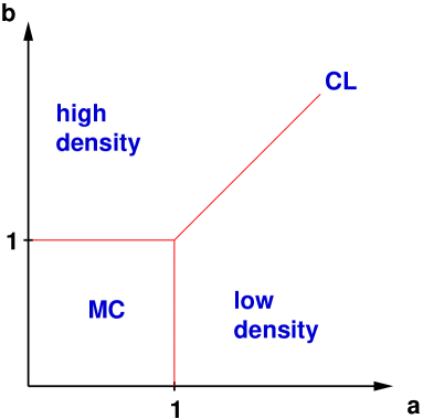
The phase diagram of the PASEP at stationarity was found by Sandow [10] and is depicted in Figureย 2. The standard phase diagram is understood to depend only on the parameters a๐‘Ža and b๐‘b defined in (2.2) rather than p,q,ฮฑ,ฮฒ,ฮณ,ฮด๐‘๐‘ž๐›ผ๐›ฝ๐›พ๐›ฟp,q,\alpha,\beta,\gamma,\delta separately, see e.g. the recent review [6]. However, we will show below that the picture may be more nuanced in the regime where ฮฑ,ฮฒโ‰ชฮณ,ฮดformulae-sequencemuch-less-than๐›ผ๐›ฝ๐›พ๐›ฟ\alpha,\beta\ll\gamma,\delta.

Refer to caption

Figure 2: Stationary state phase diagram of the PASEP. The high and low density phases are separated by the coexistence line (CL). The maximum current phase (MC) occurs at small values of the parameters a๐‘Ža and b๐‘b defined in (2.2).

Many quantities of interest, such as density profiles and currents, have been calculated for particular limits of the PASEP. For the most general case these have been computed by [25, 26].

2.2 Reverse bias

Much less is known for the case of reverse bias. The stationary state normalisation and current for ฮฑ=ฮฒ=0๐›ผ๐›ฝ0\alpha=\beta=0 have been computed by [13]. It is found that the current decays exponentially as

J=(1โˆ’qโˆ’1)โ€‹(ฮณโ€‹ฮด(1โˆ’q+ฮณ)โ€‹(1โˆ’q+ฮด))1/2โ€‹qL/2โˆ’1/4.๐ฝ1superscript๐‘ž1superscript๐›พ๐›ฟ1๐‘ž๐›พ1๐‘ž๐›ฟ12superscript๐‘ž๐ฟ214J=(1-q^{-1})\left(\frac{\gamma\delta}{(1-q+\gamma)(1-q+\delta)}\right)^{1/2}q^{L/2-1/4}. (2.3)

It was argued in [13] that non-zero values of ฮฑ๐›ผ\alpha and ฮฒ๐›ฝ\beta would allow for a right flowing current of particles to be sustained, thus destroying the reverse bias phase. However, in the following we will see that when ฮฑ๐›ผ\alpha and ฮฒ๐›ฝ\beta are ๐’ชโ€‹(qm)๐’ชsuperscript๐‘ž๐‘š\mathcal{O}(q^{m}) for some m>0๐‘š0m>0, the system still feels the effects of a reverse bias in its relaxation rates. It would be interesting to know whether such effects survive in the stationary state.

3 Relaxation rates โ€“ approach to stationarity

The slowest relaxation towards the stationary state at asymptotically late times t๐‘กt is given by eโ„ฐ1โ€‹tsuperscriptesubscriptโ„ฐ1๐‘ก{\rm e}^{\mathcal{E}_{1}t}, where โ„ฐ1subscriptโ„ฐ1\mathcal{E}_{1} is the eigenvalue of the transition matrix M๐‘€M with the largest non-zero real part.

It is well-known that the PASEP can be mapped onto the spin-1/2 anisotropic Heisenberg chain with general (integrable) open boundary conditions [10, 11]. By building on recent progress in applying the Bethe ansatz to the diagonalisation of the Hamiltonian of the latter problem [27, 28, 29], the Bethe ansatz equations for the PASEP with the most general open boundary conditions can be obtained. Recently these equations have also been derived directly using a (matrix) coordinate Bethe anstaz in the PASEP [30, 31]. The Bethe ansatz equations diagonalise the PASEP transition matrix. By analysing this set of equations for large, finite L๐ฟL the eigenvalue of the transition matrix with the largest non-zero real part has been obtained in the forward bias regime [22, 23, 24]. In this regime, particles diffuse predominantly from left to right and particle injection and extraction occurs mainly at sites 111 and L๐ฟL respectively. We will briefly review these results.

3.1 Bethe ansatz equations

As was shown in [22, 23, 24], all eigenvalues โ„ฐโ„ฐ{\cal E} of M๐‘€M other than โ„ฐ=0โ„ฐ0{\cal E}=0 can be expressed in terms of the roots zjsubscript๐‘ง๐‘—z_{j} of a set of Lโˆ’1๐ฟ1L-1 non-linear algebraic equations as

โ„ฐ=โˆ’โ„ฐ0โˆ’โˆ‘j=1Lโˆ’1ฮตโ€‹(zj),โ„ฐsubscriptโ„ฐ0superscriptsubscript๐‘—1๐ฟ1๐œ€subscript๐‘ง๐‘—\displaystyle{\mathcal{E}}=-\mathcal{E}_{0}-\sum_{j=1}^{L-1}\varepsilon(z_{j}), (3.1)

where

โ„ฐ0=ฮฑ+ฮฒ+ฮณ+ฮด=(1โˆ’q)โ€‹(1โˆ’aโ€‹c(1+a)โ€‹(1+c)+1โˆ’bโ€‹d(1+b)โ€‹(1+d)),subscriptโ„ฐ0๐›ผ๐›ฝ๐›พ๐›ฟ1๐‘ž1๐‘Ž๐‘1๐‘Ž1๐‘1๐‘๐‘‘1๐‘1๐‘‘\mathcal{E}_{0}=\alpha+\beta+\gamma+\delta=(1-q)\left(\frac{1-ac}{(1+a)(1+c)}+\frac{1-bd}{(1+b)(1+d)}\right), (3.2)

and the โ€œbare energyโ€ ฮตโ€‹(z)๐œ€๐‘ง\varepsilon(z) is

ฮตโ€‹(z)=(qโˆ’1)2โ€‹z(1โˆ’z)โ€‹(qโ€‹zโˆ’1)=(1โˆ’q)โ€‹(1zโˆ’1โˆ’1qโ€‹zโˆ’1).๐œ€๐‘งsuperscript๐‘ž12๐‘ง1๐‘ง๐‘ž๐‘ง11๐‘ž1๐‘ง11๐‘ž๐‘ง1\varepsilon(z)=\frac{(q-1)^{2}z}{(1-z)(qz-1)}=(1-q)\left(\frac{1}{z-1}-\frac{1}{qz-1}\right). (3.3)

The complex roots zjsubscript๐‘ง๐‘—z_{j} satisfy the Bethe ansatz equations

[qโ€‹zjโˆ’11โˆ’zj]2โ€‹Lโ€‹Kโ€‹(zj)=โˆlโ‰ jLโˆ’1qโ€‹zjโˆ’zlzjโˆ’qโ€‹zlโ€‹q2โ€‹zjโ€‹zlโˆ’1zjโ€‹zlโˆ’1,j=1โ€‹โ€ฆโ€‹Lโˆ’1.formulae-sequencesuperscriptdelimited-[]๐‘žsubscript๐‘ง๐‘—11subscript๐‘ง๐‘—2๐ฟ๐พsubscript๐‘ง๐‘—superscriptsubscriptproduct๐‘™๐‘—๐ฟ1๐‘žsubscript๐‘ง๐‘—subscript๐‘ง๐‘™subscript๐‘ง๐‘—๐‘žsubscript๐‘ง๐‘™superscript๐‘ž2subscript๐‘ง๐‘—subscript๐‘ง๐‘™1subscript๐‘ง๐‘—subscript๐‘ง๐‘™1๐‘—1โ€ฆ๐ฟ1\displaystyle\left[\frac{qz_{j}-1}{1-z_{j}}\right]^{2L}K(z_{j})=\prod_{l\neq j}^{L-1}\frac{qz_{j}-z_{l}}{z_{j}-qz_{l}}\frac{q^{2}z_{j}z_{l}-1}{z_{j}z_{l}-1},\ j=1\ldots L-1.
(3.4)

Here Kโ€‹(z)๐พ๐‘งK(z) is defined by

Kโ€‹(z)=(z+a)โ€‹(z+c)(qโ€‹aโ€‹z+1)โ€‹(qโ€‹cโ€‹z+1)โ€‹(z+b)โ€‹(z+d)(qโ€‹bโ€‹z+1)โ€‹(qโ€‹dโ€‹z+1),๐พ๐‘ง๐‘ง๐‘Ž๐‘ง๐‘๐‘ž๐‘Ž๐‘ง1๐‘ž๐‘๐‘ง1๐‘ง๐‘๐‘ง๐‘‘๐‘ž๐‘๐‘ง1๐‘ž๐‘‘๐‘ง1K(z)=\frac{(z+a)(z+c)}{(qaz+1)(qcz+1)}\frac{(z+b)(z+d)}{(qbz+1)(qdz+1)}, (3.5)

and a,b,c,d๐‘Ž๐‘๐‘๐‘‘a,b,c,d are given in (2.2).

3.1.1 Analysis in the forward bias regime

The analysis of the Bethe equations for the forward bias regime proceeds along the following lines. One first defines the counting function,

iโ€‹YLโ€‹(z)=gโ€‹(z)+1Lโ€‹gbโ€‹(z)+1Lโ€‹โˆ‘l=1Lโˆ’1Kโ€‹(zl,z),isubscript๐‘Œ๐ฟ๐‘ง๐‘”๐‘ง1๐ฟsubscript๐‘”b๐‘ง1๐ฟsuperscriptsubscript๐‘™1๐ฟ1๐พsubscript๐‘ง๐‘™๐‘ง{\rm i}Y_{L}(z)=g(z)+\frac{1}{L}g_{\rm b}(z)+\frac{1}{L}\sum_{l=1}^{L-1}K(z_{l},z), (3.6)

where

gโ€‹(z)๐‘”๐‘ง\displaystyle g(z) =\displaystyle= lnโก(zโ€‹(1โˆ’qโ€‹z)2(zโˆ’1)2),๐‘งsuperscript1๐‘ž๐‘ง2superscript๐‘ง12\displaystyle\ln\left(\frac{z(1-qz)^{2}}{(z-1)^{2}}\right),
gbโ€‹(z)subscript๐‘”b๐‘ง\displaystyle g_{\rm b}(z) =\displaystyle= lnโก(zโ€‹(1โˆ’q2โ€‹z2)1โˆ’z2)+lnโก(z+a1+qโ€‹aโ€‹zโ€‹1+c/z1+qโ€‹cโ€‹z)๐‘ง1superscript๐‘ž2superscript๐‘ง21superscript๐‘ง2๐‘ง๐‘Ž1๐‘ž๐‘Ž๐‘ง1๐‘๐‘ง1๐‘ž๐‘๐‘ง\displaystyle\ln\left(\frac{z(1-q^{2}z^{2})}{1-z^{2}}\right)+\ln\left(\frac{z+a}{1+qaz}\frac{1+c/z}{1+qcz}\right) (3.7)
+lnโก(z+b1+qโ€‹bโ€‹zโ€‹1+d/z1+qโ€‹dโ€‹z),๐‘ง๐‘1๐‘ž๐‘๐‘ง1๐‘‘๐‘ง1๐‘ž๐‘‘๐‘ง\displaystyle{}+\ln\left(\frac{z+b}{1+qbz}\frac{1+d/z}{1+qdz}\right),
Kโ€‹(w,z)๐พ๐‘ค๐‘ง\displaystyle K(w,z) =\displaystyle= โˆ’lnโก(w)โˆ’lnโก(1โˆ’qโ€‹z/w1โˆ’qโ€‹w/zโ€‹1โˆ’q2โ€‹zโ€‹w1โˆ’wโ€‹z).๐‘ค1๐‘ž๐‘ง๐‘ค1๐‘ž๐‘ค๐‘ง1superscript๐‘ž2๐‘ง๐‘ค1๐‘ค๐‘ง\displaystyle-\ln(w)-\ln\left(\frac{1-qz/w}{1-qw/z}\frac{1-q^{2}zw}{1-wz}\right).

We note that the choice of branch cuts in this definition of Kโ€‹(w,z)๐พ๐‘ค๐‘งK(w,z) differs from [24], but is numerically stable for large L๐ฟL. A further discussion on the choice of branch cuts in K๐พK is given in Sectionย 4.2.

Using the counting function, the Bethe ansatz equations (3.4) can be cast in logarithmic form as

YLโ€‹(zj)=2โ€‹ฯ€Lโ€‹Ij,j=1,โ€ฆ,Lโˆ’1,formulae-sequencesubscript๐‘Œ๐ฟsubscript๐‘ง๐‘—2๐œ‹๐ฟsubscript๐ผ๐‘—๐‘—1โ€ฆ๐ฟ1Y_{L}(z_{j})=\frac{2\pi}{L}I_{j}\ ,\qquad j=1,\ldots,L-1, (3.8)

where Ijsubscript๐ผ๐‘—I_{j} are integers. Each set of integers {Ij|j=1,โ€ฆ,Lโˆ’1}conditional-setsubscript๐ผ๐‘—๐‘—1โ€ฆ๐ฟ1\{I_{j}|\;j=1,\ldots,L-1\} in (3.8) specifies a particular (excited) eigenstate of the transition matrix.

In [24], the logarithmic Bethe equations were solved numerically to find the structure of the root distribution (an example of such a solution will be seen in the next section). By comparing the resulting eigenvalues with brute force diagonalisation of the transition matrix, the integers Ijsubscript๐ผ๐‘—I_{j} corresponding to the first excited state can be found for small values of L๐ฟL. The integers were found to be

Ij=โˆ’L/2+jforj=1,โ€ฆ,Lโˆ’1.formulae-sequencesubscript๐ผ๐‘—๐ฟ2๐‘—for๐‘—1โ€ฆ๐ฟ1I_{j}=-L/2+j\quad{\rm for}\quad j=1,\ldots,L-1. (3.9)

Assuming (3.9) holds for all L๐ฟL, (3.8) can be turned into an integro-differential equation for the counting function YLโ€‹(z)subscript๐‘Œ๐ฟ๐‘งY_{L}(z), which can be solved asymptotically in the limit of large L๐ฟL. Exact asymptotic expressions were obtained for the first excited eigenvalue in the forward bias regime in all areas of the stationary phase diagram except the maximal current phase. We recall here the expression for the coexistence line:

โ„ฐ1=1โˆ’qL2โ€‹ฯ€2(aโˆ’1โˆ’a)+๐’ชโ€‹(Lโˆ’3).subscriptโ„ฐ11๐‘žsuperscript๐ฟ2superscript๐œ‹2superscript๐‘Ž1๐‘Ž๐’ชsuperscript๐ฟ3\mathcal{E}_{1}=\frac{1-q}{L^{2}}\frac{\pi^{2}}{(a^{-1}-a)}+\mathcal{O}(L^{-3}). (3.10)

3.2 Dynamical phase diagram

Refer to caption

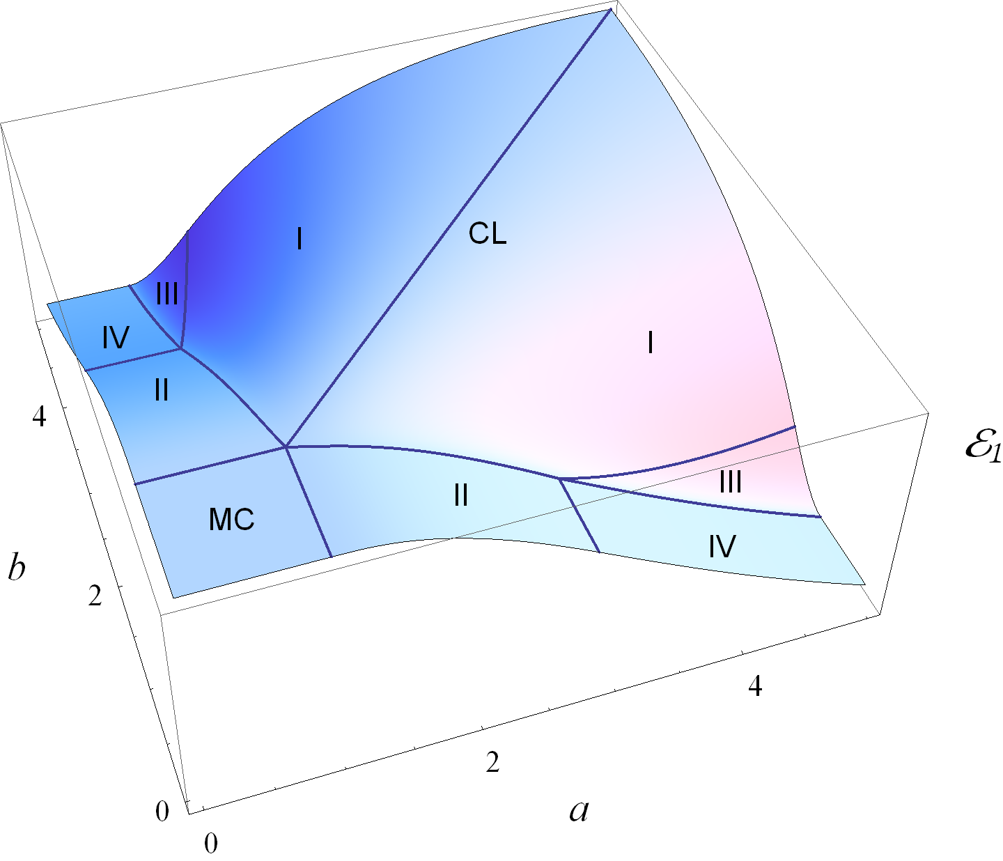
Figure 3: Dynamical phase diagram of the PASEP in the forward bias regime determined by the lowest excitation โ„ฐ1subscriptโ„ฐ1\mathcal{E}_{1}. The horizontal axes are the boundary parameters a๐‘Ža and b๐‘b (2.2) and the vertical axis is the lowest relaxation rate. The latter goes to zero for large systems on the coexistence line (CL) and in the maximum current phase (MC). The curves and lines correspond to various crossovers in the low and high density phase, across which the relaxation rate changes non-analytically.

The dynamical phase diagram for the PASEP resulting from an analysis in the regime q<1๐‘ž1q<1 is shown in Figureย 3. It exhibits the same subdivision found from the analysis of the current in the stationary state: low and high density phases (a>1๐‘Ž1a>1 and b>1๐‘1b>1) with dynamic exponent z=0๐‘ง0z=0, the coexistence line (a=b>1๐‘Ž๐‘1a=b>1) with diffusive (z=2๐‘ง2z=2) behaviour and the maximum current phase (a,b<1๐‘Ž๐‘1a,b<1) with KPZ (z=3/2๐‘ง32z=3/2) universality. Furthermore, the finite-size scaling of the lowest excited state energy of the transition matrix suggests the sub-division of both low and high-density phases into four regions respectively. These regions are characterized by different functional forms of the relaxation rates at asymptotically late times [24], see also [32].

4 Bethe ansatz in the reverse bias regime

The reverse bias regime corresponds to taking parameters a๐‘Ža, b๐‘b large, and c๐‘c, d๐‘‘d towards โˆ’11-1 (note that โˆ’1<c,dโ‰ค0formulae-sequence1๐‘๐‘‘0-1<c,d\leq 0). This change, and the resulting changes in the structure of the root distribution, requires a reformulation of the counting function, which will be discussed in Sectionย 4.2 and A. But first we describe the changes to the root structure. In the following we address solutions on the coexistence line, a=b๐‘Ž๐‘a=b, and to simplify computations further also set c=d๐‘๐‘‘c=d.

Refer to caption
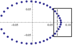
Figure 4: Root distribution in the forward bias regime for L=40๐ฟ40L=40, with parameters a=b=11๐‘Ž๐‘11a=b=11, q=0.3๐‘ž0.3q=0.3 and c=โˆ’0.07๐‘0.07c=-0.07. The dashed line marks the position of โˆ’c๐‘-c and the region in the box is expanded in Figure 5(a) below.
Refer to caption
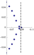
(a) c=โˆ’0.07๐‘0.07c=-0.07
Refer to caption
(b) c=โˆ’0.088๐‘0.088c=-0.088
Refer to caption
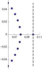
(c) c=โˆ’0.1๐‘0.1c=-0.1
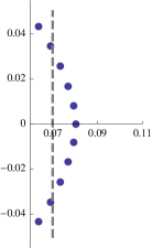
Figure 5: Leading part of the root distribution for L=40๐ฟ40L=40, a=b=11๐‘Ž๐‘11a=b=11, q=0.3๐‘ž0.3q=0.3, with c=โˆ’0.07๐‘0.07c=-0.07 (forward bias), c=โˆ’0.088๐‘0.088c=-0.088 (intermediate stage), and c=โˆ’0.1๐‘0.1c=-0.1 (reverse bias). The dashed line shows the position of โˆ’c๐‘-c.

Moving from the forward to the reverse bias regime, the structure of the Bethe roots changes. From a forward bias root distribution (Figures 4, 5(a)), increasing โˆ’c๐‘-c pushes out a complex conjugate pair of roots along with the single root on the positive real axis (Figure 5(b)). As โˆ’c๐‘-c increases further, the complex conjugate pair pinch in to the real axis until some point where they โ€œcollapseโ€ (Figure 5(c)) โ€“ one root returns to close the contour on the positive real axis leaving an isolated pair of real roots at

zยฑ=โˆ’cยฑeโˆ’ฮฝยฑโ€‹L,ฮฝยฑ>0.formulae-sequencesuperscript๐‘งplus-or-minusplus-or-minus๐‘superscript๐‘’superscript๐œˆplus-or-minus๐ฟsuperscript๐œˆplus-or-minus0z^{\pm}=-c\pm e^{-\nu^{\pm}L},\quad\nu^{\pm}>0. (4.1)

In fact, there is a pair of isolated roots for all kโˆˆโ„•๐‘˜โ„•k\in\mathbb{N} such that โˆ’qkโ€‹csuperscript๐‘ž๐‘˜๐‘-q^{k}c falls outside the contour of complex roots.

For L๐ฟL large, the contour crosses the real axis at [24]

zโˆ—โ€‹(a)=1+4โ€‹a+a2โˆ’(1+4โ€‹a+a2)2โˆ’4โ€‹a22โ€‹aโ‰ƒ1a,superscript๐‘ง๐‘Ž14๐‘Žsuperscript๐‘Ž2superscript14๐‘Žsuperscript๐‘Ž224superscript๐‘Ž22๐‘Žsimilar-to-or-equals1๐‘Žz^{*}(a)=\frac{1+4a+a^{2}-\sqrt{(1+4a+a^{2})^{2}-4a^{2}}}{2a}\simeq\frac{1}{a}, (4.2)

where the approximation is for a๐‘Ža large. Therefore, the integer m๐‘šm defined by a๐‘Ža and c๐‘c through the inequalities

โˆ’qmโ€‹c<1a<โˆ’qmโˆ’1โ€‹c,superscript๐‘ž๐‘š๐‘1๐‘Žsuperscript๐‘ž๐‘š1๐‘-q^{m}c<\frac{1}{a}<-q^{m-1}c, (4.3)

is equal to the maximum number of pairs of real roots as Lโ†’โˆžโ†’๐ฟL\to\infty. While we take our parameters to have generic values, it would be of interest to analyse the system at the resonant values of a๐‘Ža, c๐‘c where the inequalities become equalities, see e.g. [33].

Refer to caption
Refer to caption
Figure 6: Complete root distribution (top) and zoomed in on the contour and first few pairs of isolated roots (bottom) for L=100๐ฟ100L=100, aยฏ=3.09ยฏ๐‘Ž3.09\bar{a}=3.09, c=โˆ’0.9๐‘0.9c=-0.9, q=0.3๐‘ž0.3q=0.3 and m=20๐‘š20m=20 (at this resolution only five real pairs are visible in the top figure).

We define

aยฏ=qmโˆ’1โ€‹a,ยฏ๐‘Žsuperscript๐‘ž๐‘š1๐‘Ž\bar{a}=q^{m-1}a, (4.4)

then, for example, we will reach a maximum m=20๐‘š20m=20 pairs of real roots with the parameters

aยฏ=3.09,c=โˆ’0.9,q=0.3.formulae-sequenceยฏ๐‘Ž3.09formulae-sequence๐‘0.9๐‘ž0.3\bar{a}=3.09,\quad c=-0.9,\quad q=0.3. (4.5)

The corresponding root distribution is displayed in Figureย 6.

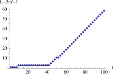
We denote by mโ€ฒsuperscript๐‘šโ€ฒm^{\prime} the number of pairs of real roots for a particular value of L๐ฟL, with mโ€ฒโ‰คmsuperscript๐‘šโ€ฒ๐‘šm^{\prime}\leq m. Then the number of roots on the contour is Lโˆ’2โ€‹mโ€ฒโˆ’1๐ฟ2superscript๐‘šโ€ฒ1L-2m^{\prime}-1, which is plotted in Figure 7 for the parameters (4.5). There are three regions to consider:

  1. 1.

    Isolated roots region: Lโˆ’2โ€‹mโ€ฒโˆ’1๐ฟ2superscript๐‘šโ€ฒ1L-2m^{\prime}-1 small and almost all roots occur as isolated pairs;

  2. 2.

    Crossover region: The contour of complex roots begins to form, mโ€ฒโ‰ƒmsimilar-to-or-equalssuperscript๐‘šโ€ฒ๐‘šm^{\prime}\simeq m;

  3. 3.

    Asymptotic region: The number of roots on the contour, Lโˆ’2โ€‹mโ€ฒโˆ’1๐ฟ2superscript๐‘šโ€ฒ1L-2m^{\prime}-1 is large.

Refer to caption
Figure 7: Number of complex roots in the contour (Lโˆ’2โ€‹mโ€ฒโˆ’1๐ฟ2superscript๐‘šโ€ฒ1L-2m^{\prime}-1) against L๐ฟL. Only beyond L=40๐ฟ40L=40 does the contour of complex roots begin to form.

4.1 Isolated roots region

We first consider the case where Lโˆ’2โ€‹mโ€ฒโˆ’1๐ฟ2superscript๐‘šโ€ฒ1L-2m^{\prime}-1 is small and assume all roots are real, a situation similar to that encountered in the recent calculation of the PASEP current fluctuations [34]. The mโ€ฒsuperscript๐‘šโ€ฒm^{\prime} pairs of isolated roots are

zkยฑ=โˆ’qkโ€‹cยฑeโˆ’ฮฝkยฑโ€‹Lk=0,โ€ฆ,mโ€ฒโˆ’1,formulae-sequencesuperscriptsubscript๐‘ง๐‘˜plus-or-minusplus-or-minussuperscript๐‘ž๐‘˜๐‘superscript๐‘’superscriptsubscript๐œˆ๐‘˜plus-or-minus๐ฟ๐‘˜0โ€ฆsuperscript๐‘šโ€ฒ1z_{k}^{\pm}=-q^{k}c\pm e^{-\nu_{k}^{\pm}L}\qquad k=0,\ldots,m^{\prime}-1, (4.6)

and the remaing root is close to โˆ’qmโ€‹csuperscript๐‘ž๐‘š๐‘-q^{m}c. Substituting these roots into the expression for the eigenvalue (3.1) and dropping exponentially small parts, the sum telescopes, leaving

โ„ฐ1(is)=โˆ’(1โˆ’q)โ€‹2โ€‹qmโˆ’1qmโˆ’1+aยฏโˆ’(1โˆ’q)โ€‹qmโ€ฒโˆ’1โ€‹(โˆ’qโ€‹c1+qmโ€ฒโ€‹c+โˆ’q2โ€‹c1+qmโ€ฒ+1โ€‹c).superscriptsubscriptโ„ฐ1is1๐‘ž2superscript๐‘ž๐‘š1superscript๐‘ž๐‘š1ยฏ๐‘Ž1๐‘žsuperscript๐‘žsuperscript๐‘šโ€ฒ1๐‘ž๐‘1superscript๐‘žsuperscript๐‘šโ€ฒ๐‘superscript๐‘ž2๐‘1superscript๐‘žsuperscript๐‘šโ€ฒ1๐‘\mathcal{E}_{1}^{\rm{(is)}}=-(1-q)\frac{2q^{m-1}}{q^{m-1}+\bar{a}}-(1-q)q^{m^{\prime}-1}\left(\frac{-qc}{1+q^{m^{\prime}}c}+\frac{-q^{2}c}{1+q^{m^{\prime}+1}c}\right). (4.7)

The L๐ฟL dependence enters through mโ€ฒsuperscript๐‘šโ€ฒm^{\prime} and implies that the eigenvalue decays as qL/2superscript๐‘ž๐ฟ2q^{L/2} to a constant, which is ๐’ชโ€‹(qm)๐’ชsuperscript๐‘ž๐‘š\mathcal{O}\left(q^{m}\right). This differs markedly from the asymptotic expression in the forward bias regime (3.10).

4.2 Asymptotic region

We now analyse the third region, where the number of roots on the contour is large. As we are interested in the asymptotic behaviour, we will assume we have reached the maximum number of pairs of real roots (mโ€ฒ=msuperscript๐‘šโ€ฒ๐‘šm^{\prime}=m). We label the roots on the contour

zj,j=1โ€‹โ€ฆโ€‹Lโˆ’2โ€‹mโˆ’1,subscript๐‘ง๐‘—๐‘—1โ€ฆ๐ฟ2๐‘š1\displaystyle z_{j},\quad j=1\ldots L-2m-1, (4.8)

and the real roots, as before, as

zkยฑ=โˆ’qkโ€‹cยฑeโˆ’ฮฝkยฑโ€‹L,ฮฝkยฑ>0,k=0,โ€ฆ,mโˆ’1.formulae-sequencesuperscriptsubscript๐‘ง๐‘˜plus-or-minusplus-or-minussuperscript๐‘ž๐‘˜๐‘superscriptesuperscriptsubscript๐œˆ๐‘˜plus-or-minus๐ฟformulae-sequencesuperscriptsubscript๐œˆ๐‘˜plus-or-minus0๐‘˜0โ€ฆ๐‘š1\displaystyle z_{k}^{\pm}=-q^{k}c\pm{\rm e}^{-\nu_{k}^{\pm}L},\qquad\nu_{k}^{\pm}>0,\qquad k=0,\ldots,m-1. (4.9)

The choice of branch cuts in the counting function (3.6), (3.7) is suitable for the forward bias regime. In the reverse bias regime we must redefine the counting function. The form we use is

iโ€‹YLโ€‹(z)isubscript๐‘Œ๐ฟ๐‘ง\displaystyle{\rm i}Y_{L}(z) =\displaystyle= gโ€‹(z)+1Lโ€‹gbโ€‹(z)+1Lโ€‹โˆ‘l=0mโˆ’1(Krโ€‹(zlโˆ’,z)+Krโ€‹(zl+,z))๐‘”๐‘ง1๐ฟsubscript๐‘”b๐‘ง1๐ฟsuperscriptsubscript๐‘™0๐‘š1subscript๐พrsuperscriptsubscript๐‘ง๐‘™๐‘งsubscript๐พrsuperscriptsubscript๐‘ง๐‘™๐‘ง\displaystyle g(z)+\frac{1}{L}g_{\rm b}(z)+\frac{1}{L}\sum_{l=0}^{m-1}\left(K_{\rm{r}}(z_{l}^{-},z)+K_{\rm{r}}(z_{l}^{+},z)\right) (4.10)
+1Lโ€‹โˆ‘l=1Lโˆ’2โ€‹mโˆ’1Kโ€‹(zl,z)1๐ฟsuperscriptsubscript๐‘™1๐ฟ2๐‘š1๐พsubscript๐‘ง๐‘™๐‘ง\displaystyle\hskip 71.13188pt+\frac{1}{L}\sum_{l=1}^{L-2m-1}K(z_{l},z)

where now

gโ€‹(z)๐‘”๐‘ง\displaystyle g(z) =\displaystyle= lnโก(zโ€‹(1โˆ’qโ€‹z)2(1โˆ’z)2),๐‘งsuperscript1๐‘ž๐‘ง2superscript1๐‘ง2\displaystyle\ln\left(\frac{z(1-qz)^{2}}{(1-z)^{2}}\right),
gbโ€‹(z)subscript๐‘”b๐‘ง\displaystyle g_{\rm b}(z) =\displaystyle= lnโก(1โˆ’q2โ€‹z2zโ€‹(1โˆ’z2))+2โ€‹lnโก(cโ€‹qmโˆ’1โ€‹z+aยฏqmโˆ’1+qโ€‹aยฏโ€‹zโ€‹1+z/c1+qโ€‹cโ€‹z),1superscript๐‘ž2superscript๐‘ง2๐‘ง1superscript๐‘ง22๐‘superscript๐‘ž๐‘š1๐‘งยฏ๐‘Žsuperscript๐‘ž๐‘š1๐‘žยฏ๐‘Ž๐‘ง1๐‘ง๐‘1๐‘ž๐‘๐‘ง\displaystyle\ln\left(\frac{1-q^{2}z^{2}}{z(1-z^{2})}\right)+2\ln\left(c\frac{q^{m-1}z+\bar{a}}{q^{m-1}+q\bar{a}z}\frac{1+z/c}{1+qcz}\right),
Kโ€‹(w,z)๐พ๐‘ค๐‘ง\displaystyle K(w,z) =\displaystyle= โˆ’lnโก(1โˆ’qโ€‹z/w1โˆ’qโ€‹w/zโ€‹1โˆ’q2โ€‹zโ€‹w1โˆ’zโ€‹w)โˆ’lnโกw,1๐‘ž๐‘ง๐‘ค1๐‘ž๐‘ค๐‘ง1superscript๐‘ž2๐‘ง๐‘ค1๐‘ง๐‘ค๐‘ค\displaystyle-\ln\left(\frac{1-qz/w}{1-qw/z}\frac{1-q^{2}zw}{1-zw}\right)-\ln w, (4.11)
Krโ€‹(w,z)subscript๐พr๐‘ค๐‘ง\displaystyle K_{\rm{r}}(w,z) =\displaystyle= โˆ’lnโก(1โˆ’qโˆ’1โ€‹w/z1โˆ’qโ€‹w/zโ€‹1โˆ’q2โ€‹wโ€‹z1โˆ’wโ€‹z)โˆ’lnโก(qโ€‹z).1superscript๐‘ž1๐‘ค๐‘ง1๐‘ž๐‘ค๐‘ง1superscript๐‘ž2๐‘ค๐‘ง1๐‘ค๐‘ง๐‘ž๐‘ง\displaystyle-\ln\left(\frac{1-q^{-1}w/z}{1-qw/z}\frac{1-q^{2}wz}{1-wz}\right)-\ln(qz).

With this definition, the complex roots satisfy

YLโ€‹(zj)=2โ€‹ฯ€Lโ€‹Ij,j=1,โ€ฆ,Lโˆ’2โ€‹mโˆ’1,formulae-sequencesubscript๐‘Œ๐ฟsubscript๐‘ง๐‘—2๐œ‹๐ฟsubscript๐ผ๐‘—๐‘—1โ€ฆ๐ฟ2๐‘š1Y_{L}(z_{j})=\frac{2\pi}{L}I_{j},\quad j=1,\ldots,L-2m-1, (4.12)

with the integers Ijsubscript๐ผ๐‘—I_{j} that correspond to the first excited state given by

Ij=โˆ’(L2โˆ’m)+j.subscript๐ผ๐‘—๐ฟ2๐‘š๐‘—I_{j}=-\left(\frac{L}{2}-m\right)+j. (4.13)

The real roots satisfy

YLโ€‹(zkยฑ)=2โ€‹ฯ€Lโ€‹Ikยฑ,k=0,โ€ฆ,mโˆ’1,formulae-sequencesubscript๐‘Œ๐ฟsuperscriptsubscript๐‘ง๐‘˜plus-or-minus2๐œ‹๐ฟsuperscriptsubscript๐ผ๐‘˜plus-or-minus๐‘˜0โ€ฆ๐‘š1Y_{L}(z_{k}^{\pm})=\frac{2\pi}{L}I_{k}^{\pm},\qquad k=0,\ldots,m-1, (4.14)

but the Ikยฑsuperscriptsubscript๐ผ๐‘˜plus-or-minusI_{k}^{\pm} are not distinct. To find numerical solutions, we use an alternative form of the counting function that numbers all roots consecutively (see A). However, the form (4.10), (4.11) is better suited to the following asymptotic analysis.

4.2.1 Counting function for the complex roots

We can account for the contribution of the isolated roots in (4.12) and obtain Bethe equations for the complex roots alone. Ignoring exponentially small parts, the sum over real roots in (4.10) telescopes,

โˆ‘l=0mโˆ’1(Krโ€‹(zlโˆ’,z)+Krโ€‹(zl+,z))superscriptsubscript๐‘™0๐‘š1subscript๐พ๐‘Ÿsuperscriptsubscript๐‘ง๐‘™๐‘งsubscript๐พ๐‘Ÿsuperscriptsubscript๐‘ง๐‘™๐‘ง\displaystyle\sum_{l=0}^{m-1}\Bigg{(}K_{r}(z_{l}^{-},z)+K_{r}(z_{l}^{+},z)\Bigg{)} (4.15)
โ‰ƒsimilar-to-or-equals\displaystyle\simeq โˆ’2โ€‹mโ€‹lnโก(qโ€‹z)+2โ€‹lnโก[(1+zqmโ€‹c)โ€‹(1+zqmโˆ’1โ€‹c)โ€‹(c+qโ€‹z)]2๐‘š๐‘ž๐‘ง21๐‘งsuperscript๐‘ž๐‘š๐‘1๐‘งsuperscript๐‘ž๐‘š1๐‘๐‘๐‘ž๐‘ง\displaystyle-2m\ln(qz)+2\ln\left[\left(1+\frac{z}{q^{m}c}\right)\left(1+\frac{z}{q^{m-1}c}\right)\left(c+qz\right)\right]
โˆ’lnโก(z+c)โˆ’lnโก[(1+qm+1โ€‹cโ€‹z)โ€‹(1+qmโ€‹cโ€‹z)(1+qโ€‹cโ€‹z)โ€‹(1+cโ€‹z)].๐‘ง๐‘1superscript๐‘ž๐‘š1๐‘๐‘ง1superscript๐‘ž๐‘š๐‘๐‘ง1๐‘ž๐‘๐‘ง1๐‘๐‘ง\displaystyle\hskip 14.22636pt-\ln(z+c)-\ln\left[\frac{(1+q^{m+1}cz)(1+q^{m}cz)}{(1+qcz)(1+cz)}\right].

The complex roots lie on a simple curve in the complex plane, which approaches a closed contour as Lโ†’โˆžโ†’๐ฟL\rightarrow\infty. From (4.2) and (4.4), we see that the size of the contour scales as qmโˆ’1superscript๐‘ž๐‘š1q^{m-1}. We therefore change to the scaled variables

z=qmโˆ’1โ€‹ฮถ,๐‘งsuperscript๐‘ž๐‘š1๐œz=q^{m-1}\zeta, (4.16)

and take into account the 2โ€‹m2๐‘š2m real roots โ€œmissingโ€ from the contour by defining a new counting function

YยฏLโˆ’2โ€‹mโ€‹(ฮถ)=LLโˆ’2โ€‹mโ€‹YLโ€‹(qmโˆ’1โ€‹ฮถ).subscriptยฏ๐‘Œ๐ฟ2๐‘š๐œ๐ฟ๐ฟ2๐‘šsubscript๐‘Œ๐ฟsuperscript๐‘ž๐‘š1๐œ\overline{Y}_{L-2m}(\zeta)=\frac{L}{L-2m}Y_{L}(q^{m-1}\zeta). (4.17)

With the change to the scaled variables ฮถ๐œ\zeta, we may drop any ๐’ชโ€‹(qm)๐’ชsuperscript๐‘ž๐‘š\mathcal{O}(q^{m}) contributions. For example,

gโ€‹(z)=gโ€‹(qmโˆ’1โ€‹ฮถ)๐‘”๐‘ง๐‘”superscript๐‘ž๐‘š1๐œ\displaystyle g(z)=g(q^{m-1}\zeta) =\displaystyle= (mโˆ’1)โ€‹lnโกq+lnโก(ฮถโ€‹(1โˆ’qmโ€‹ฮถ)2(1โˆ’qmโˆ’1โ€‹ฮถ)2)๐‘š1๐‘ž๐œsuperscript1superscript๐‘ž๐‘š๐œ2superscript1superscript๐‘ž๐‘š1๐œ2\displaystyle(m-1)\ln q+\ln\left(\frac{\zeta(1-q^{m}\zeta)^{2}}{(1-q^{m-1}\zeta)^{2}}\right) (4.18)
โ‰ƒsimilar-to-or-equals\displaystyle\simeq (mโˆ’1)โ€‹lnโกq+lnโกฮถ.๐‘š1๐‘ž๐œ\displaystyle(m-1)\ln q+\ln\zeta.

Collecting terms by order of 1/(Lโˆ’2โ€‹m)1๐ฟ2๐‘š1/(L-2m), the new counting function is given by

iโ€‹YยฏLโˆ’2โ€‹mโ€‹(ฮถ)=gยฏโ€‹(ฮถ)+1Lโˆ’2โ€‹mโ€‹gยฏbโ€‹(ฮถ)+1Lโˆ’2โ€‹mโ€‹โˆ‘l=1Lโˆ’2โ€‹mโˆ’1Kยฏโ€‹(ฮถl,ฮถ),isubscriptยฏ๐‘Œ๐ฟ2๐‘š๐œยฏ๐‘”๐œ1๐ฟ2๐‘šsubscriptยฏ๐‘”b๐œ1๐ฟ2๐‘šsuperscriptsubscript๐‘™1๐ฟ2๐‘š1ยฏ๐พsubscript๐œ๐‘™๐œ{\rm i}\overline{Y}_{L-2m}(\zeta)=\bar{g}(\zeta)+\frac{1}{L-2m}\bar{g}_{\rm b}(\zeta)+\frac{1}{L-2m}\sum_{l=1}^{L-2m-1}\overline{K}(\zeta_{l},\zeta), (4.19)

with

gยฏโ€‹(ฮถ)ยฏ๐‘”๐œ\displaystyle\bar{g}(\zeta) =lnโกฮถabsent๐œ\displaystyle=\ln\zeta
gยฏbโ€‹(ฮถ)subscriptยฏ๐‘”b๐œ\displaystyle\bar{g}_{\rm b}(\zeta) =โˆ’lnโก(ฮถ)+2โ€‹lnโก(aยฏโ€‹ฮถ1+qโ€‹aยฏโ€‹ฮถ)+2โ€‹lnโก(ฮถ+qโ€‹c)+2โ€‹lnโก(1+ฮถc),absent๐œ2ยฏ๐‘Ž๐œ1๐‘žยฏ๐‘Ž๐œ2๐œ๐‘ž๐‘21๐œ๐‘\displaystyle=-\ln(\zeta)+2\ln\left(\frac{\bar{a}\zeta}{1+q\bar{a}\zeta}\right)+2\ln\left(\zeta+qc\right)+2\ln\left(1+\frac{\zeta}{c}\right), (4.20)
Kยฏโ€‹(ฯ‰,ฮถ)ยฏ๐พ๐œ”๐œ\displaystyle\overline{K}(\omega,\zeta) =โˆ’lnโก(1โˆ’qโ€‹ฮถ/ฯ‰1โˆ’qโ€‹ฯ‰/ฮถ)โˆ’lnโก(ฯ‰),absent1๐‘ž๐œ๐œ”1๐‘ž๐œ”๐œ๐œ”\displaystyle=-\ln\left(\frac{1-q\zeta/\omega}{1-q\omega/\zeta}\right)-\ln(\omega),

where we recall that aยฏยฏ๐‘Ž\bar{a} is defined in (4.4). The telescoped sum (4.15) contributes terms to both gยฏยฏ๐‘”\bar{g} and gยฏbsubscriptยฏ๐‘”b\bar{g}_{\rm b}. The Bethe ansatz equations for the scaled complex roots are

YยฏLโˆ’2โ€‹mโ€‹(ฮถj)=2โ€‹ฯ€Lโˆ’2โ€‹mโ€‹Ij,j=1,โ€ฆ,Lโˆ’2โ€‹mโˆ’1,formulae-sequencesubscriptยฏ๐‘Œ๐ฟ2๐‘šsubscript๐œ๐‘—2๐œ‹๐ฟ2๐‘šsubscript๐ผ๐‘—๐‘—1โ€ฆ๐ฟ2๐‘š1\overline{Y}_{L-2m}(\zeta_{j})=\frac{2\pi}{L-2m}I_{j},\quad j=1,\dots,L-2m-1, (4.21)

with

Ij=โˆ’Lโˆ’2โ€‹m2+j.subscript๐ผ๐‘—๐ฟ2๐‘š2๐‘—I_{j}=-\frac{L-2m}{2}+j. (4.22)

The eigenvalue, in terms of the scaled roots ฮถjsubscript๐œ๐‘—\zeta_{j} is

โ„ฐ1(rev)=โˆ’โ„ฐ0(rev)โˆ’โˆ‘l=1Lโˆ’2โ€‹mโˆ’1ฮตยฏโ€‹(ฮถl),superscriptsubscriptโ„ฐ1(rev)superscriptsubscriptโ„ฐ0revsuperscriptsubscript๐‘™1๐ฟ2๐‘š1ยฏ๐œ€subscript๐œ๐‘™\mathcal{E}_{1}^{\textrm{(rev)}}=-\mathcal{E}_{0}^{(\textrm{rev})}-\sum_{l=1}^{L-2m-1}\bar{\varepsilon}(\zeta_{l}), (4.23)

where

โ„ฐ0(rev)=โˆ’2โ€‹(1โˆ’q)โ€‹qmโˆ’1โ€‹(1qmโˆ’1+aยฏโˆ’qโ€‹c1+qmโ€‹c),superscriptsubscriptโ„ฐ0rev21๐‘žsuperscript๐‘ž๐‘š11superscript๐‘ž๐‘š1ยฏ๐‘Ž๐‘ž๐‘1superscript๐‘ž๐‘š๐‘\mathcal{E}_{0}^{(\textrm{rev})}=-2(1-q)q^{m-1}\left(\frac{1}{q^{m-1}+\bar{a}}-\frac{qc}{1+q^{m}c}\right), (4.24)

includes โ„ฐ0subscriptโ„ฐ0\mathcal{E}_{0} and the contribution from the real roots, and the scaled bare energy is

ฮตยฏโ€‹(ฮถ)=โˆ’(1โˆ’q)2โ€‹qmโˆ’1โ€‹ฮถ(1โˆ’qmโˆ’1โ€‹ฮถ)โ€‹(1โˆ’qmโ€‹ฮถ).ยฏ๐œ€๐œsuperscript1๐‘ž2superscript๐‘ž๐‘š1๐œ1superscript๐‘ž๐‘š1๐œ1superscript๐‘ž๐‘š๐œ\bar{\varepsilon}(\zeta)=-(1-q)^{2}q^{m-1}\frac{\zeta}{\left(1-q^{m-1}\zeta\right)\left(1-q^{m}\zeta\right)}. (4.25)

5 Asymptotic Analysis

The equations (4.21) are logarithmic Bethe equations for the complex roots in the reverse bias regime. These equations have the same form as the forward bias equations (3.6) with the key difference that there are now Lโˆ’2โ€‹mโˆ’1๐ฟ2๐‘š1L-2m-1 roots instead of Lโˆ’1๐ฟ1L-1 (recall that m๐‘šm is defined by the condition (4.3)). The method used in [24] to derive exact large L๐ฟL asymptotics for the eigenvalue โ„ฐ1subscriptโ„ฐ1\mathcal{E}_{1} can be applied to the reverse bias regime. But we require now that Lโˆ’2โ€‹m๐ฟ2๐‘šL-2m is large.

Refer to caption
Figure 8: Integration contour enclosing the complex roots.

As a simple consequence of the residue theorem we can write

1Lโˆ’2โ€‹mโ€‹โˆ‘j=1Lโˆ’2โ€‹mโˆ’1fโ€‹(ฮถi)1๐ฟ2๐‘šsuperscriptsubscript๐‘—1๐ฟ2๐‘š1๐‘“subscript๐œ๐‘–\displaystyle\frac{1}{L-2m}\sum_{j=1}^{L-2m-1}f(\zeta_{i}) =\displaystyle= (5.1)
โˆฎC1+C2dโ€‹ฮถ4โ€‹ฯ€โ€‹iโ€‹fโ€‹(ฮถ)โ€‹YยฏLโˆ’2โ€‹mโ€ฒโ€‹(ฮถ)โ€‹cotโก(12โ€‹(Lโˆ’2โ€‹m)โ€‹YยฏLโˆ’2โ€‹mโ€‹(ฮถ)),subscriptcontour-integralsubscript๐ถ1subscript๐ถ2๐‘‘๐œ4๐œ‹i๐‘“๐œsubscriptsuperscriptยฏ๐‘Œโ€ฒ๐ฟ2๐‘š๐œ12๐ฟ2๐‘šsubscriptยฏ๐‘Œ๐ฟ2๐‘š๐œ\displaystyle\oint_{C_{1}+C_{2}}\frac{d\zeta}{4\pi{\rm i}}f(\zeta)\overline{Y}^{\prime}_{L-2m}(\zeta)\cot\left(\frac{1}{2}(L-2m)\overline{Y}_{L-2m}(\zeta)\right),

where C=C1+C2๐ถsubscript๐ถ1subscript๐ถ2C=C_{1}+C_{2} is a contour enclosing all the complex roots ฮถjsubscript๐œ๐‘—\zeta_{j} (see Figure 8) and fโ€‹(ฮถ)๐‘“๐œf(\zeta) is a function analytic inside C๐ถC. We will use (5.1) to write an integro-differential equation for the counting function YยฏLโˆ’2โ€‹mโ€‹(ฮถ)subscriptยฏ๐‘Œ๐ฟ2๐‘š๐œ\overline{Y}_{L-2m}(\zeta), but first we note some properties of YยฏLโˆ’2โ€‹mโ€‹(ฮถ)subscriptยฏ๐‘Œ๐ฟ2๐‘š๐œ\overline{Y}_{L-2m}(\zeta).

The complex roots ฮถjsubscript๐œ๐‘—\zeta_{j} are connected by the contour Imโ€‹[YยฏLโˆ’2โ€‹mโ€‹(ฮถ)]=0Imdelimited-[]subscriptยฏ๐‘Œ๐ฟ2๐‘š๐œ0\textrm{Im}\left[\overline{Y}_{L-2m}(\zeta)\right]=0. This contour extends to a point on the negative real axis, ฮถcsubscript๐œc\zeta_{\rm c}. We fix ฮพ๐œ‰\xi and ฮพโˆ—superscript๐œ‰\xi^{*}, the endpoints of C1subscript๐ถ1C_{1} and C2subscript๐ถ2C_{2}, on this contour by

YยฏLโˆ’2โ€‹mโ€‹(ฮพโˆ—)=โˆ’ฯ€+ฯ€Lโˆ’2โ€‹m,YยฏLโˆ’2โ€‹mโ€‹(ฮพ)=ฯ€โˆ’ฯ€Lโˆ’2โ€‹m.formulae-sequencesubscriptยฏ๐‘Œ๐ฟ2๐‘šsuperscript๐œ‰๐œ‹๐œ‹๐ฟ2๐‘šsubscriptยฏ๐‘Œ๐ฟ2๐‘š๐œ‰๐œ‹๐œ‹๐ฟ2๐‘š\overline{Y}_{L-2m}(\xi^{*})=-\pi+\frac{\pi}{L-2m},\quad\overline{Y}_{L-2m}(\xi)=\pi-\frac{\pi}{L-2m}. (5.2)

On C1subscript๐ถ1C_{1}, inside the contour connecting the roots, the imaginary part of YยฏLโˆ’2โ€‹mโ€‹(ฮถ)subscriptยฏ๐‘Œ๐ฟ2๐‘š๐œ\overline{Y}_{L-2m}(\zeta) is positive; on C2subscript๐ถ2C_{2} it is negative.

Using (5.1) in (4.19), we obtain a non-linear integro-differential equation for YยฏLโˆ’2โ€‹mโ€‹(ฮถ)subscriptยฏ๐‘Œ๐ฟ2๐‘š๐œ\overline{Y}_{L-2m}(\zeta), which, using the properties just described, is written as an integral over the contour of roots from ฮพโˆ—superscript๐œ‰\xi^{*} to ฮพ๐œ‰\xi, and correction terms integrated over C1subscript๐ถ1C_{1} and C2subscript๐ถ2C_{2}:

iโ€‹YยฏLโˆ’2โ€‹mโ€‹(ฮถ)isubscriptยฏ๐‘Œ๐ฟ2๐‘š๐œ\displaystyle{\rm i}\,\overline{Y}_{L-2m}(\zeta) =\displaystyle= gยฏโ€‹(ฮถ)+1Lโˆ’2โ€‹mโ€‹gยฏbโ€‹(ฮถ)+12โ€‹ฯ€โ€‹โˆซฮพโˆ—ฮพKยฏโ€‹(ฯ‰,ฮถ)โ€‹YยฏLโˆ’2โ€‹mโ€ฒโ€‹(ฯ‰)โ€‹dฯ‰ยฏ๐‘”๐œ1๐ฟ2๐‘šsubscriptยฏ๐‘”b๐œ12๐œ‹superscriptsubscriptsuperscript๐œ‰๐œ‰ยฏ๐พ๐œ”๐œsubscriptsuperscriptยฏ๐‘Œโ€ฒ๐ฟ2๐‘š๐œ”differential-d๐œ”\displaystyle\bar{g}(\zeta)+\frac{1}{L-2m}\bar{g}_{\rm b}(\zeta)+\frac{1}{2\pi}\int_{\xi^{*}}^{\xi}\overline{K}(\omega,\zeta)\overline{Y}^{\prime}_{L-2m}(\omega){\rm d}\omega (5.3)
+12โ€‹ฯ€โ€‹โˆซC1Kยฏโ€‹(ฯ‰,ฮถ)โ€‹YยฏLโˆ’2โ€‹mโ€ฒโ€‹(ฯ‰)1โˆ’eโˆ’iโ€‹(Lโˆ’2โ€‹m)โ€‹YยฏLโˆ’2โ€‹mโ€‹(ฯ‰)โ€‹dฯ‰12๐œ‹subscriptsubscript๐ถ1ยฏ๐พ๐œ”๐œsubscriptsuperscriptยฏ๐‘Œโ€ฒ๐ฟ2๐‘š๐œ”1superscriptei๐ฟ2๐‘šsubscriptยฏ๐‘Œ๐ฟ2๐‘š๐œ”differential-d๐œ”\displaystyle+\frac{1}{2\pi}\int_{C_{1}}\frac{\overline{K}(\omega,\zeta)\overline{Y}^{\prime}_{L-2m}(\omega)}{1-{\rm e}^{-{\rm i}(L-2m)\overline{Y}_{L-2m}(\omega)}}\,{\rm d}\omega
+12โ€‹ฯ€โ€‹โˆซC2Kยฏโ€‹(ฯ‰,ฮถ)โ€‹YยฏLโˆ’2โ€‹mโ€ฒโ€‹(ฯ‰)eiโ€‹(Lโˆ’2โ€‹m)โ€‹YยฏLโˆ’2โ€‹mโ€‹(ฯ‰)โˆ’1โ€‹dฯ‰.12๐œ‹subscriptsubscript๐ถ2ยฏ๐พ๐œ”๐œsubscriptsuperscriptยฏ๐‘Œโ€ฒ๐ฟ2๐‘š๐œ”superscriptei๐ฟ2๐‘šsubscriptยฏ๐‘Œ๐ฟ2๐‘š๐œ”1differential-d๐œ”\displaystyle+\frac{1}{2\pi}\int_{C_{2}}\frac{\overline{K}(\omega,\zeta)\overline{Y}^{\prime}_{L-2m}(\omega)}{{\rm e}^{{\rm i}(L-2m)\overline{Y}_{L-2m}(\omega)}-1}\,{\rm d}\omega.

The correction terms can be approximated as in [24] giving

iโ€‹YยฏLโˆ’2โ€‹mโ€‹(ฮถ)isubscriptยฏ๐‘Œ๐ฟ2๐‘š๐œ\displaystyle{\rm i}\,\overline{Y}_{L-2m}(\zeta) =\displaystyle= gยฏโ€‹(ฮถ)+1Lโˆ’2โ€‹mโ€‹gยฏbโ€‹(ฮถ)+12โ€‹ฯ€โ€‹โˆซฮถcโˆ’ฮถc+Kยฏโ€‹(ฯ‰,ฮถ)โ€‹YยฏLโˆ’2โ€‹mโ€ฒโ€‹(ฯ‰)โ€‹dฯ‰ยฏ๐‘”๐œ1๐ฟ2๐‘šsubscriptยฏ๐‘”b๐œ12๐œ‹superscriptsubscriptsuperscriptsubscript๐œcsuperscriptsubscript๐œcยฏ๐พ๐œ”๐œsubscriptsuperscriptยฏ๐‘Œโ€ฒ๐ฟ2๐‘š๐œ”differential-d๐œ”\displaystyle\bar{g}(\zeta)+\frac{1}{L-2m}\bar{g}_{\rm b}(\zeta)+\frac{1}{2\pi}\int_{\zeta_{\rm c}^{-}}^{\zeta_{\rm c}^{+}}\overline{K}(\omega,\zeta)\overline{Y}^{\prime}_{L-2m}(\omega){\rm d}\omega (5.4)
+12โ€‹ฯ€โ€‹โˆซฮพโˆ—ฮถcโˆ’Kยฏโ€‹(ฯ‰,ฮถ)โ€‹YยฏLโˆ’2โ€‹mโ€ฒโ€‹(ฯ‰)โ€‹dฯ‰+12โ€‹ฯ€โ€‹โˆซฮถc+ฮพKยฏโ€‹(ฯ‰,ฮถ)โ€‹YยฏLโˆ’2โ€‹mโ€ฒโ€‹(ฯ‰)โ€‹dฯ‰12๐œ‹superscriptsubscriptsuperscript๐œ‰superscriptsubscript๐œcยฏ๐พ๐œ”๐œsubscriptsuperscriptยฏ๐‘Œโ€ฒ๐ฟ2๐‘š๐œ”differential-d๐œ”12๐œ‹superscriptsubscriptsuperscriptsubscript๐œc๐œ‰ยฏ๐พ๐œ”๐œsubscriptsuperscriptยฏ๐‘Œโ€ฒ๐ฟ2๐‘š๐œ”differential-d๐œ”\displaystyle{}+\frac{1}{2\pi}\int_{\xi^{*}}^{\zeta_{\rm c}^{-}}\overline{K}(\omega,\zeta)\overline{Y}^{\prime}_{L-2m}(\omega){\rm d}\omega+\frac{1}{2\pi}\int_{\zeta_{\rm c}^{+}}^{\xi}\overline{K}(\omega,\zeta)\overline{Y}^{\prime}_{L-2m}(\omega){\rm d}\omega
+ฯ€12โ€‹(Lโˆ’2โ€‹m)2โ€‹(Kยฏโ€ฒโ€‹(ฮพโˆ—,ฮถ)YยฏLโˆ’2โ€‹mโ€ฒโ€‹(ฮพโˆ—)โˆ’Kยฏโ€ฒโ€‹(ฮพ,ฮถ)YยฏLโˆ’2โ€‹mโ€ฒโ€‹(ฮพ))+๐’ชโ€‹(1(Lโˆ’2โ€‹m)4).๐œ‹12superscript๐ฟ2๐‘š2superscriptยฏ๐พโ€ฒsuperscript๐œ‰๐œsubscriptsuperscriptยฏ๐‘Œโ€ฒ๐ฟ2๐‘šsuperscript๐œ‰superscriptยฏ๐พโ€ฒ๐œ‰๐œsubscriptsuperscriptยฏ๐‘Œโ€ฒ๐ฟ2๐‘š๐œ‰๐’ช1superscript๐ฟ2๐‘š4\displaystyle{}+\frac{\pi}{12(L-2m)^{2}}\left(\frac{\overline{K}^{\prime}(\xi^{*},\zeta)}{\overline{Y}^{\prime}_{L-2m}(\xi^{*})}-\frac{\overline{K}^{\prime}(\xi,\zeta)}{\overline{Y}^{\prime}_{L-2m}(\xi)}\right)+\mathcal{O}\left(\frac{1}{(L-2m)^{4}}\right).

Here, the derivatives of Kยฏยฏ๐พ\overline{K} are with respect to the first argument, and we have extended the integration contour beyond the endpoints, so that it pinches the negative real axis at points ฮถcยฑ=ฮถcยฑi0superscriptsubscript๐œcplus-or-minusplus-or-minussubscript๐œci0\zeta_{\rm c}^{\pm}=\zeta_{\rm c}\pm{\rm i}0.

Equation (5.4) is solved as follows. We Taylor expand the integrands of the integrals from ฮพโˆ—superscript๐œ‰\xi^{*} to ฮถcโˆ’superscriptsubscript๐œ๐‘\zeta_{c}^{-} and from ฮถc+superscriptsubscript๐œc\zeta_{\rm c}^{+} to ฮพ๐œ‰\xi. Then we substitute the expansions

YยฏLโˆ’2โ€‹mโ€‹(ฮถ)=โˆ‘n=0โˆž(Lโˆ’2โ€‹m)โˆ’nโ€‹ynโ€‹(ฮถ),ฮพ=ฮถc+โˆ‘n=1โˆž(Lโˆ’2โ€‹m)โˆ’nโ€‹(ฮดn+iโ€‹ฮทn)formulae-sequencesubscriptยฏ๐‘Œ๐ฟ2๐‘š๐œsuperscriptsubscript๐‘›0superscript๐ฟ2๐‘š๐‘›subscript๐‘ฆ๐‘›๐œ๐œ‰subscript๐œ๐‘superscriptsubscript๐‘›1superscript๐ฟ2๐‘š๐‘›subscript๐›ฟ๐‘›๐‘–subscript๐œ‚๐‘›\overline{Y}_{L-2m}(\zeta)=\sum_{n=0}^{\infty}(L-2m)^{-n}y_{n}(\zeta),\quad\xi=\zeta_{c}+\sum_{n=1}^{\infty}(L-2m)^{-n}(\delta_{n}+i\eta_{n}) (5.5)

and expand in inverse powers of Lโˆ’2โ€‹m๐ฟ2๐‘šL-2m. This yields a hierarchy of integro-differential equations for the functions ynโ€‹(ฮถ)subscript๐‘ฆ๐‘›๐œy_{n}(\zeta)

ynโ€‹(ฮถ)=gnโ€‹(ฮถ)+12โ€‹ฯ€โ€‹iโ€‹โˆซฮถcโˆ’ฮถc+Kยฏโ€‹(ฯ‰,ฮถ)โ€‹ynโ€ฒโ€‹(ฯ‰)โ€‹๐‘‘ฯ‰.subscript๐‘ฆ๐‘›๐œsubscript๐‘”๐‘›๐œ12๐œ‹isuperscriptsubscriptsuperscriptsubscript๐œcsuperscriptsubscript๐œcยฏ๐พ๐œ”๐œsubscriptsuperscript๐‘ฆโ€ฒ๐‘›๐œ”differential-d๐œ”y_{n}(\zeta)=g_{n}(\zeta)+\frac{1}{2\pi{\rm i}}\int_{\zeta_{\rm c}^{-}}^{\zeta_{\rm c}^{+}}\overline{K}(\omega,\zeta)y^{\prime}_{n}(\omega)\,d\omega. (5.6)

The integral is along the closed contour following the locus of roots. The first few driving terms gnโ€‹(ฮถ)subscript๐‘”๐‘›๐œg_{n}(\zeta) are given by

g0โ€‹(ฮถ)=โˆ’iโ€‹gยฏโ€‹(ฮถ),g1โ€‹(ฮถ)=โˆ’iโ€‹gยฏbโ€‹(ฮถ)+ฮบ1+ฮป1โ€‹Kยฏ~โ€‹(ฮถc,ฮถ),g2โ€‹(ฮถ)=ฮบ2+ฮป2โ€‹Kยฏ~โ€‹(ฮถc,ฮถ)+ฮผ2โ€‹Kยฏโ€ฒโ€‹(ฮถc,ฮถ),g3โ€‹(ฮถ)=ฮบ3+ฮป3โ€‹Kยฏ~โ€‹(ฮถc,ฮถ)+ฮผ3โ€‹Kยฏโ€ฒโ€‹(ฮถc,ฮถ)+ฮฝ3โ€‹Kยฏโ€ฒโ€ฒโ€‹(ฮถc,ฮถ).subscript๐‘”0๐œiยฏ๐‘”๐œsubscript๐‘”1๐œisubscriptยฏ๐‘”b๐œsubscript๐œ…1subscript๐œ†1~ยฏ๐พsubscript๐œc๐œsubscript๐‘”2๐œsubscript๐œ…2subscript๐œ†2~ยฏ๐พsubscript๐œc๐œsubscript๐œ‡2superscriptยฏ๐พโ€ฒsubscript๐œc๐œsubscript๐‘”3๐œsubscript๐œ…3subscript๐œ†3~ยฏ๐พsubscript๐œc๐œsubscript๐œ‡3superscriptยฏ๐พโ€ฒsubscript๐œc๐œsubscript๐œˆ3superscriptยฏ๐พโ€ฒโ€ฒsubscript๐œc๐œ\begin{array}[]{r@{\hspace{2pt}}c@{\hspace{3pt}}l}g_{0}(\zeta)\hskip 2.0&=\hfil\hskip 3.0&-{\rm i}\bar{g}(\zeta),\\ g_{1}(\zeta)\hskip 2.0&=\hfil\hskip 3.0&-{\rm i}\bar{g}_{\textrm{b}}(\zeta)+\kappa_{1}+\lambda_{1}\widetilde{\overline{K}}(\zeta_{\rm c},\zeta),\\ g_{2}(\zeta)\hskip 2.0&=\hfil\hskip 3.0&\kappa_{2}+\lambda_{2}\widetilde{\overline{K}}(\zeta_{\rm c},\zeta)+\mu_{2}\overline{K}^{\prime}(\zeta_{\rm c},\zeta),\\ g_{3}(\zeta)\hskip 2.0&=\hfil\hskip 3.0&\kappa_{3}+\lambda_{3}\widetilde{\overline{K}}(\zeta_{\rm c},\zeta)+\mu_{3}\overline{K}^{\prime}(\zeta_{\rm c},\zeta)+\nu_{3}\overline{K}^{\prime\prime}(\zeta_{\rm c},\zeta).\end{array} (5.7)

The functions gยฏโ€‹(ฮถ)ยฏ๐‘”๐œ\bar{g}(\zeta) and gbยฏโ€‹(ฮถ)ยฏsubscript๐‘”b๐œ\bar{g_{\textrm{b}}}(\zeta) are defined in (4.2.1) and (4.20), and

Kยฏ~โ€‹(ฮถc,ฮถ)=โˆ’lnโก(โˆ’ฮถc)+lnโก(1โˆ’qโ€‹ฮถc/ฮถ1โˆ’qโ€‹ฮถ/ฮถc)~ยฏ๐พsubscript๐œc๐œsubscript๐œc1๐‘žsubscript๐œc๐œ1๐‘ž๐œsubscript๐œc\widetilde{\overline{K}}(\zeta_{\rm c},\zeta)=-\ln(-\zeta_{\rm c})+\ln\left(\frac{1-q\zeta_{\rm c}/\zeta}{1-q\zeta/\zeta_{\rm c}}\right) (5.8)

arises when we evaluate Kยฏโ€‹(ฮถcยฑ,ฮถ)ยฏ๐พsuperscriptsubscript๐œcplus-or-minus๐œ\overline{K}(\zeta_{\rm c}^{\pm},\zeta) and take the limit ฮถcยฑโ†’ฮถcโ†’superscriptsubscript๐œcplus-or-minussubscript๐œc\zeta_{\rm c}^{\pm}\to\zeta_{\rm c}.

The coefficients ฮบnsubscript๐œ…๐‘›\kappa_{n}, ฮปnsubscript๐œ†๐‘›\lambda_{n}, ฮผnsubscript๐œ‡๐‘›\mu_{n} and ฮฝnsubscript๐œˆ๐‘›\nu_{n} are given in terms of ฮดnsubscript๐›ฟ๐‘›\delta_{n}, ฮฝnsubscript๐œˆ๐‘›\nu_{n}, defined by (5.5), and by derivatives of ynsubscript๐‘ฆ๐‘›y_{n} evaluated at ฮถcsubscript๐œc\zeta_{\rm c}. Explicit expressions are given in B. We note that although the definition of the counting function has changed, and despite expanding in Lโˆ’2โ€‹m๐ฟ2๐‘šL-2m instead of L๐ฟL, the form of these coefficients and the driving terms are unchanged from [24].

5.1 Solving for the ynsubscript๐‘ฆ๐‘›y_{n}

We may now solve (5.6) order by order. Working with the scaled roots, with the restrictions on parameters of the reverse bias regime we can assume that โˆ’qโ€‹c๐‘ž๐‘-qc lies inside the contour of integration, and that โˆ’1qโ€‹aยฏ1๐‘žยฏ๐‘Ž-\frac{1}{q\bar{a}} and โˆ’c๐‘-c lie outside it. The calculation follows in the same way as in [24], so we give here only the result for the counting function:

YยฏLโˆ’2โ€‹mโ€‹(ฮถ)subscriptยฏ๐‘Œ๐ฟ2๐‘š๐œ\displaystyle\overline{Y}_{L-2m}(\zeta) =\displaystyle= y0โ€‹(ฮถ)+1Lโˆ’2โ€‹mโ€‹y1โ€‹(ฮถ)+1(Lโˆ’2โ€‹m)2โ€‹y2โ€‹(ฮถ)subscript๐‘ฆ0๐œ1๐ฟ2๐‘šsubscript๐‘ฆ1๐œ1superscript๐ฟ2๐‘š2subscript๐‘ฆ2๐œ\displaystyle y_{0}(\zeta)+\frac{1}{L-2m}y_{1}(\zeta)+\frac{1}{(L-2m)^{2}}y_{2}(\zeta) (5.9)
+1(Lโˆ’2โ€‹m)3โ€‹y3โ€‹(ฮถ)+๐’ชโ€‹(1(Lโˆ’2โ€‹m)4),1superscript๐ฟ2๐‘š3subscript๐‘ฆ3๐œ๐’ช1superscript๐ฟ2๐‘š4\displaystyle+\frac{1}{(L-2m)^{3}}y_{3}(\zeta)+\mathcal{O}\left(\frac{1}{(L-2m)^{4}}\right),

where

y0โ€‹(ฮถ)subscript๐‘ฆ0๐œ\displaystyle y_{0}(\zeta) =\displaystyle= โˆ’iโ€‹lnโก(โˆ’ฮถฮถc)i๐œsubscript๐œc\displaystyle-{\rm i}\ln\left(-\frac{\zeta}{\zeta_{\rm c}}\right) (5.10)
y1โ€‹(ฮถ)subscript๐‘ฆ1๐œ\displaystyle y_{1}(\zeta) =\displaystyle= โˆ’iโ€‹lnโก(โˆ’ฮถฮถc)โˆ’2โ€‹iโ€‹lnโก(aยฏ)โˆ’ฮป1โ€‹lnโก(โˆ’ฮถc)+ฮบ1i๐œsubscript๐œc2iยฏ๐‘Žsubscript๐œ†1subscript๐œcsubscript๐œ…1\displaystyle-{\rm i}\ln\left(-\frac{\zeta}{\zeta_{\rm c}}\right)-2{\rm i}\ln\left(\bar{a}\right)-\lambda_{1}\ln(-\zeta_{\rm c})+\kappa_{1} (5.11)
โˆ’2โ€‹iโ€‹lnโก[(โˆ’qโ€‹c/ฮถ;q)โˆž(โˆ’qโ€‹c/ฮถc;q)โˆž]+ฮป1โ€‹lnโก[(qโ€‹ฮถc/ฮถ;q)โˆž(qโ€‹ฮถ/ฮถc;q)โˆž]2isubscript๐‘ž๐‘๐œ๐‘žsubscript๐‘ž๐‘subscript๐œc๐‘žsubscript๐œ†1subscript๐‘žsubscript๐œc๐œ๐‘žsubscript๐‘ž๐œsubscript๐œc๐‘ž\displaystyle-2{\rm i}\ln\left[\frac{(-qc/\zeta;q)_{\infty}}{(-qc/\zeta_{\rm c};q)_{\infty}}\right]+\lambda_{1}\ln\left[\frac{(q\zeta_{\rm c}/\zeta;q)_{\infty}}{(q\zeta/\zeta_{\rm c};q)_{\infty}}\right]
โˆ’2โ€‹iโ€‹lnโก[(โˆ’ฮถ/c;q)โˆž(โˆ’ฮถc/c;q)โˆž]2isubscript๐œ๐‘๐‘žsubscriptsubscript๐œc๐‘๐‘ž\displaystyle-2{\rm i}\ln\left[\frac{(-\zeta/c;q)_{\infty}}{(-\zeta_{\rm c}/c;q)_{\infty}}\right]
y2โ€‹(ฮถ)subscript๐‘ฆ2๐œ\displaystyle y_{2}(\zeta) =\displaystyle= ฮบ2โˆ’ฮป2โ€‹lnโก(โˆ’ฮถc)โˆ’ฮผ2ฮถc+ฮป2โ€‹lnโก[(qโ€‹ฮถc/ฮถ;q)โˆž(qโ€‹ฮถ/ฮถc;q)โˆž]+ฮผ2โ€‹ฮจ1โ€‹(ฮถ|q)subscript๐œ…2subscript๐œ†2subscript๐œcsubscript๐œ‡2subscript๐œcsubscript๐œ†2subscript๐‘žsubscript๐œc๐œ๐‘žsubscript๐‘ž๐œsubscript๐œc๐‘žsubscript๐œ‡2subscriptฮจ1conditional๐œ๐‘ž\displaystyle\kappa_{2}-\lambda_{2}\ln(-\zeta_{\rm c})-\frac{\mu_{2}}{\zeta_{\rm c}}+\lambda_{2}\ln\left[\frac{(q\zeta_{\rm c}/\zeta;q)_{\infty}}{(q\zeta/\zeta_{\rm c};q)_{\infty}}\right]+\mu_{2}\Psi_{1}(\zeta|q)
y3โ€‹(ฮถ)subscript๐‘ฆ3๐œ\displaystyle y_{3}(\zeta) =\displaystyle= ฮบ3โˆ’ฮป3โ€‹lnโก(โˆ’ฮถc)โˆ’ฮผ3ฮถc+ฮฝ3ฮถc2+ฮป3โ€‹lnโก[(qโ€‹ฮถc/ฮถ;q)โˆž(qโ€‹ฮถ/ฮถc;q)โˆž]subscript๐œ…3subscript๐œ†3subscript๐œcsubscript๐œ‡3subscript๐œcsubscript๐œˆ3superscriptsubscript๐œc2subscript๐œ†3subscript๐‘žsubscript๐œc๐œ๐‘žsubscript๐‘ž๐œsubscript๐œc๐‘ž\displaystyle\kappa_{3}-\lambda_{3}\ln(-\zeta_{\rm c})-\frac{\mu_{3}}{\zeta_{\rm c}}+\frac{\nu_{3}}{\zeta_{\rm c}^{2}}+\lambda_{3}\ln\left[\frac{(q\zeta_{\rm c}/\zeta;q)_{\infty}}{(q\zeta/\zeta_{\rm c};q)_{\infty}}\right] (5.12)
+ฮผ3โ€‹ฮจ1โ€‹(ฮถ|q)โˆ’ฮฝ3โ€‹ฮจ2โ€‹(ฮถ|q)subscript๐œ‡3subscriptฮจ1conditional๐œ๐‘žsubscript๐œˆ3subscriptฮจ2conditional๐œ๐‘ž\displaystyle+\mu_{3}\Psi_{1}(\zeta|q)-\nu_{3}\Psi_{2}(\zeta|q)

Here (a;q)โˆžsubscript๐‘Ž๐‘ž(a;q)_{\infty} denotes the q-Pochhammer symbol

(a;q)โˆž=โˆk=0โˆž(1โˆ’aโ€‹qk),subscript๐‘Ž๐‘žsuperscriptsubscriptproduct๐‘˜01๐‘Žsuperscript๐‘ž๐‘˜(a;q)_{\infty}=\prod_{k=0}^{\infty}(1-aq^{k}), (5.13)

and we have defined functions

ฮจkโ€‹(ฮถ|q)=ฯˆkโ€‹(ฮถ|qโˆ’1)โˆ’ฯˆkโ€‹(ฮถc|qโˆ’1)โˆ’(ฯˆkโ€‹(ฮถ|q)โˆ’ฯˆkโ€‹(ฮถc|q))subscriptฮจ๐‘˜conditional๐œ๐‘žsubscript๐œ“๐‘˜conditional๐œsuperscript๐‘ž1subscript๐œ“๐‘˜conditionalsubscript๐œcsuperscript๐‘ž1subscript๐œ“๐‘˜conditional๐œ๐‘žsubscript๐œ“๐‘˜conditionalsubscript๐œc๐‘ž\Psi_{k}(\zeta|q)=\psi_{k}(\zeta|q^{-1})-\psi_{k}(\zeta_{\rm c}|q^{-1})-\left(\psi_{k}(\zeta|q)-\psi_{k}(\zeta_{\rm c}|q)\right) (5.14)

with222 The definition of ฯˆkโ€‹(ฮถ|q)subscript๐œ“๐‘˜conditional๐œ๐‘ž\psi_{k}(\zeta|q) used in [24] is incorrect for expressions such as ฯˆkโ€‹(ฮถโˆ’1|qโˆ’1)subscript๐œ“๐‘˜conditionalsuperscript๐œ1superscript๐‘ž1\psi_{k}(\zeta^{-1}|q^{-1}).

ฯˆkโ€‹(ฮถ|q)=โˆ‘n=0โˆž1(ฮถcโˆ’qn+1โ€‹ฮถ)k.subscript๐œ“๐‘˜conditional๐œ๐‘žsuperscriptsubscript๐‘›01superscriptsubscript๐œcsuperscript๐‘ž๐‘›1๐œ๐‘˜\psi_{k}(\zeta|q)=\sum_{n=0}^{\infty}\frac{1}{(\zeta_{\rm c}-q^{n+1}\zeta)^{k}}\ . (5.15)

5.2 Boundary conditions

Substituting the expansions (5.5) into the boundary conditions (5.2), which fix the endpoints ฮพ๐œ‰\xi and ฮพโˆ—superscript๐œ‰\xi^{*}, we obtain a hierarchy of conditions for ynโ€‹(ฮถc)subscript๐‘ฆ๐‘›subscript๐œcy_{n}(\zeta_{\rm c}), e.g.

YยฏLโˆ’2โ€‹mโ€‹(ฮพ)subscriptยฏ๐‘Œ๐ฟ2๐‘š๐œ‰\displaystyle\overline{Y}_{L-2m}(\xi) =\displaystyle= y0โ€‹(ฮพ)+1Lโˆ’2โ€‹mโ€‹y1โ€‹(ฮพ)+1(Lโˆ’2โ€‹m)2โ€‹y2โ€‹(ฮพ)+โ€ฆsubscript๐‘ฆ0๐œ‰1๐ฟ2๐‘šsubscript๐‘ฆ1๐œ‰1superscript๐ฟ2๐‘š2subscript๐‘ฆ2๐œ‰โ€ฆ\displaystyle y_{0}(\xi)+\frac{1}{L-2m}y_{1}(\xi)+\frac{1}{(L-2m)^{2}}y_{2}(\xi)+\ldots (5.16)
=\displaystyle= y0โ€‹(ฮถc)+1Lโˆ’2โ€‹mโ€‹[y1โ€‹(ฮถc)+y0โ€ฒโ€‹(ฮถc)โ€‹(ฮด1+iโ€‹ฮท1)]+โ€ฆsubscript๐‘ฆ0subscript๐œc1๐ฟ2๐‘šdelimited-[]subscript๐‘ฆ1subscript๐œcsuperscriptsubscript๐‘ฆ0โ€ฒsubscript๐œcsubscript๐›ฟ1isubscript๐œ‚1โ€ฆ\displaystyle y_{0}(\zeta_{\rm c})+\frac{1}{L-2m}\left[y_{1}(\zeta_{\rm c})+y_{0}^{\prime}(\zeta_{\rm c})(\delta_{1}+{\rm i}\eta_{1})\right]+\ldots
=\displaystyle= ฯ€โˆ’ฯ€Lโˆ’2โ€‹m.๐œ‹๐œ‹๐ฟ2๐‘š\displaystyle\pi-\frac{\pi}{L-2m}\ .

Solving this equation order by order, we find

ฮป1=2โ€‹i,ฮถc=โˆ’1aยฏ,formulae-sequencesubscript๐œ†12isubscript๐œc1ยฏ๐‘Ž\lambda_{1}=2{\rm i},\qquad\zeta_{\rm c}=-\frac{1}{\bar{a}}, (5.17)

and

ฮป3=ฮผ2=ฮป2=ฮบ1=ฮบ2=0,ฮฝ3=ฮถcโ€‹ฮผ3=โˆ’iโ€‹ฯ€2โ€‹ฮถc.subscript๐œ†3subscript๐œ‡2subscript๐œ†2subscript๐œ…1subscript๐œ…20subscript๐œˆ3subscript๐œcsubscript๐œ‡3isuperscript๐œ‹2subscript๐œc\begin{array}[]{r@{\hspace{2pt}}c@{\hspace{3pt}}l}\lambda_{3}\hskip 2.0&=\hfil\hskip 3.0&\mu_{2}=\lambda_{2}=\kappa_{1}=\kappa_{2}=0,\\ \nu_{3}\hskip 2.0&=\hfil\hskip 3.0&\displaystyle\zeta_{\rm c}\mu_{3}=-{\rm i}\pi^{2}\zeta_{\rm c}.\end{array} (5.18)

5.3 Eigenvalue with largest non-zero real part

As was done for the counting function, we use (5.1) in (4.23) to obtain an integro-differential equation for the eigenvalue. Evaluating the resulting integrals in the same way as for the counting function itself, we obtain

โ„ฐ=โˆ’โ„ฐ0(rev)โˆ’Lโˆ’2โ€‹m2โ€‹ฯ€โ€‹โˆฎฮถcฮตยฏโ€‹(ฮถ)โ€‹YยฏLโˆ’2โ€‹mโ€ฒโ€‹(ฮถ)โ€‹๐‘‘ฮถโˆ’iโ€‹โˆ‘nโ‰ฅ0enโ€‹(Lโˆ’2โ€‹m)โˆ’n,โ„ฐsuperscriptsubscriptโ„ฐ0(rev)๐ฟ2๐‘š2๐œ‹subscriptcontour-integralsubscript๐œcยฏ๐œ€๐œsuperscriptsubscriptยฏ๐‘Œ๐ฟ2๐‘šโ€ฒ๐œdifferential-d๐œisubscript๐‘›0subscript๐‘’๐‘›superscript๐ฟ2๐‘š๐‘›\mathcal{E}=-\mathcal{E}_{0}^{\textrm{(rev)}}-\frac{L-2m}{2\pi}\oint_{\zeta_{\rm c}}\bar{\varepsilon}(\zeta)\overline{Y}_{L-2m}^{\prime}(\zeta)\,d\zeta-{\rm i}\sum_{n\geq 0}e_{n}(L-2m)^{-n}, (5.19)

where the integral is over the closed contour on which the roots lie, โ„ฐ0(rev)superscriptsubscriptโ„ฐ0(rev)\mathcal{E}_{0}^{\textrm{(rev)}} and ฮตยฏยฏ๐œ€\bar{\varepsilon} are given in (4.24) and (4.25), and

e0subscript๐‘’0\displaystyle e_{0} =\displaystyle= ฮป1โ€‹ฮตยฏโ€‹(ฮถc),subscript๐œ†1ยฏ๐œ€subscript๐œc\displaystyle\lambda_{1}\bar{\varepsilon}(\zeta_{\rm c}),
e1subscript๐‘’1\displaystyle e_{1} =\displaystyle= ฮป2โ€‹ฮตยฏโ€‹(ฮถc)+ฮผ2โ€‹ฮตยฏโ€ฒโ€‹(ฮถc),subscript๐œ†2ยฏ๐œ€subscript๐œcsubscript๐œ‡2superscriptยฏ๐œ€โ€ฒsubscript๐œc\displaystyle\lambda_{2}\bar{\varepsilon}(\zeta_{\rm c})+\mu_{2}\bar{\varepsilon}^{\prime}(\zeta_{\rm c}), (5.20)
e2subscript๐‘’2\displaystyle e_{2} =\displaystyle= ฮป3โ€‹ฮตยฏโ€‹(ฮถc)+ฮผ3โ€‹ฮตยฏโ€ฒโ€‹(ฮถc)+ฮฝ3โ€‹ฮตยฏโ€ฒโ€ฒโ€‹(ฮถc).subscript๐œ†3ยฏ๐œ€subscript๐œcsubscript๐œ‡3superscriptยฏ๐œ€โ€ฒsubscript๐œcsubscript๐œˆ3superscriptยฏ๐œ€โ€ฒโ€ฒsubscript๐œc\displaystyle\lambda_{3}\bar{\varepsilon}(\zeta_{\rm c})+\mu_{3}\bar{\varepsilon}^{\prime}(\zeta_{\rm c})+\nu_{3}\bar{\varepsilon}^{\prime\prime}(\zeta_{\rm c}).

Substituting the expansion (5.9) for YยฏLโˆ’2โ€‹mโ€‹(ฮถ)subscriptยฏ๐‘Œ๐ฟ2๐‘š๐œ\overline{Y}_{L-2m}(\zeta) into (5.19) we arrive at the following result for the eigenvalue of the transition matrix with the largest non-zero real part

โ„ฐ1(rev)=qmโˆ’1(Lโˆ’2โ€‹m)2โ€‹ฯ€2โ€‹(1โˆ’q)โ€‹aยฏq2โ€‹(mโˆ’1)โˆ’aยฏ2+๐’ชโ€‹(1(Lโˆ’2โ€‹m)3).superscriptsubscriptโ„ฐ1(rev)superscript๐‘ž๐‘š1superscript๐ฟ2๐‘š2superscript๐œ‹21๐‘žยฏ๐‘Žsuperscript๐‘ž2๐‘š1superscriptยฏ๐‘Ž2๐’ช1superscript๐ฟ2๐‘š3\mathcal{E}_{1}^{\textrm{(rev)}}=\frac{q^{m-1}}{(L-2m)^{2}}\frac{\pi^{2}(1-q)\bar{a}}{q^{2(m-1)}-\bar{a}^{2}}+\mathcal{O}\left(\frac{1}{(L-2m)^{3}}\right). (5.21)

Making the substitution aยฏ=qmโˆ’1โ€‹aยฏ๐‘Žsuperscript๐‘ž๐‘š1๐‘Ž\bar{a}=q^{m-1}a, we see that this is

โ„ฐ1(rev)=1(Lโˆ’2โ€‹m)2โ€‹ฯ€2โ€‹(1โˆ’q)aโˆ’1โˆ’a+๐’ชโ€‹(1(Lโˆ’2โ€‹m)3),superscriptsubscriptโ„ฐ1(rev)1superscript๐ฟ2๐‘š2superscript๐œ‹21๐‘žsuperscript๐‘Ž1๐‘Ž๐’ช1superscript๐ฟ2๐‘š3\mathcal{E}_{1}^{\textrm{(rev)}}=\frac{1}{(L-2m)^{2}}\frac{\pi^{2}(1-q)}{a^{-1}-a}+\mathcal{O}\left(\frac{1}{(L-2m)^{3}}\right), (5.22)

which differs from the expression in the forward bias regime (3.10) only by changing Lโ†’Lโˆ’2โ€‹mโ†’๐ฟ๐ฟ2๐‘šL\to L-2m. In Sectionย 7 we discuss the physical interpretation of this result.

6 Crossover region

We have found two very different expressions for the eigenvalue: โ„ฐ1(is)superscriptsubscriptโ„ฐ1(is)\mathcal{E}_{1}^{\textrm{(is)}} in (4.7) describing the relaxation for relatively small L๐ฟL, dominated by the isolated real roots, and โ„ฐ1(rev)superscriptsubscriptโ„ฐ1(rev)\mathcal{E}_{1}^{\textrm{(rev)}} in (5.21) describing the asymptotic relaxation when Lโˆ’2โ€‹m๐ฟ2๐‘šL-2m is large. As L๐ฟL increases, the contour of complex roots begins to form. The first approximation is no longer valid, and the second cannot be applied until the contour is sufficiently large.

Nevertheless, we can compare the magnitude of the two expressions in this region. Assuming mโ€ฒ=msuperscript๐‘šโ€ฒ๐‘šm^{\prime}=m, we can approximate (4.7) as

โ„ฐ1(is)โ‰ƒโˆ’qmโˆ’1โ€‹(1โˆ’q)โ€‹(2aยฏโˆ’(1+q)โ€‹qโ€‹c).similar-to-or-equalssuperscriptsubscriptโ„ฐ1(is)superscript๐‘ž๐‘š11๐‘ž2ยฏ๐‘Ž1๐‘ž๐‘ž๐‘\mathcal{E}_{1}^{\textrm{(is)}}\simeq-q^{m-1}(1-q)\left(\frac{2}{\bar{a}}-(1+q)qc\right). (6.1)

The asymptotic expression (5.21) can be approximated as

โ„ฐ1(rev)โ‰ƒโˆ’qmโˆ’1โ€‹(1โˆ’q)โ€‹ฯ€2(Lโˆ’2โ€‹m)2โ€‹1aยฏ.similar-to-or-equalssuperscriptsubscriptโ„ฐ1(rev)superscript๐‘ž๐‘š11๐‘žsuperscript๐œ‹2superscript๐ฟ2๐‘š21ยฏ๐‘Ž\mathcal{E}_{1}^{\textrm{(rev)}}\simeq-q^{m-1}(1-q)\frac{\pi^{2}}{(L-2m)^{2}}\frac{1}{\bar{a}}. (6.2)

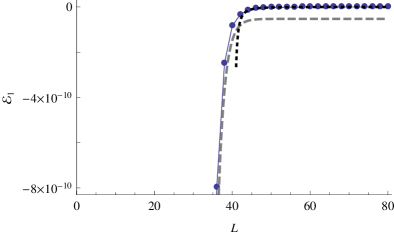
The contour begins to form when Lโˆ’2โ€‹m=2๐ฟ2๐‘š2L-2m=2, and at this point we see that the two expressions are comparable. Figure 9 shows the two expressions and the numerically calculated value in the crossover region.
Refer to caption
Figure 9: โ„ฐ1(is)superscriptsubscriptโ„ฐ1(is)\mathcal{E}_{1}^{\textrm{(is)}} (dashed), โ„ฐ1(rev)superscriptsubscriptโ„ฐ1(rev)\mathcal{E}_{1}^{\textrm{(rev)}} (dotted), and numerical value (datapoints connected by thin solid line) for m=20๐‘š20m=20 and parameters (4.5).

7 Conclusion

We have computed the relaxation rate on the coexistence line of the partially asymmetric exclusion process with reverse biased boundary rates. Such rates introduce a length scale mโ‰ˆโˆ’logโก(โˆ’aโ€‹c)/logโกq๐‘š๐‘Ž๐‘๐‘žm\approx-\log(-ac)/\log q in the system, determined by (4.3). There are two distinct sub regimes. When the system size is small compared to the reverse bias, i.e. Lโ‰ฒ2โ€‹mless-than-or-similar-to๐ฟ2๐‘šL\lesssim 2m, the relaxation is exponential in the system size and the inverse relaxation time is given by (4.7). For large systems, Lโ‰ซ2โ€‹mmuch-greater-than๐ฟ2๐‘šL\gg 2m, the relaxation on the coexistence line is diffusive but the inverse relaxation time vanishes with the square of a reduced system size Lโˆ’2โ€‹m๐ฟ2๐‘šL-2m. This behaviour can be obtained by an effective one particle diffusion model as in [23, 35] but in a reduced system of size Lโˆ’2โ€‹m๐ฟ2๐‘šL-2m.

We thus observe the effects of the reverse bias on the relaxation rate even with non-zero (but small) rates in the forward direction โ€“ provided the rates in the reverse direction are large enough. We suspect that in this case the forward contribution to the stationary current of particles is not strong enough to destroy the reverse bias phase, contrary to the argument in [13]. It would be of interest to revisit the calculation of the stationary current to see whether this is indeed the case.

The corresponding physical interpretation of these results is the following. In the setup of this paper, where the bulk bias is from left to right, the system will fill up completely on the right hand side over a length 2โ€‹m2๐‘š2m. In the remaining space of size Lโˆ’2โ€‹m๐ฟ2๐‘šL-2m, the system behaves as a regular PASEP on the coexistence line, and forms a uniformly distributed domain wall. As far as we are aware, the stationary density profile of the PASEP in the reverse bias regime has not been computed analytically, and it would be interesting to see whether this picture is confirmed by such a calculation.

Acknowledgments

Our warm thanks goes to Fabian Essler for discussions. Financial assistance from the Australian Research Council is gratefully acknowledged.

Appendix A Numerical solutions of the Bethe equations

The logarithmic form of the Bethe equations is numerically stable for large L๐ฟL, as long as an appropriate form of the counting function is used. In the forward bias regime, that form is (3.6). For the reverse bias regime the situation is more complicated. The form (4.10) is suited to the asymptotic analysis โ€“ by assuming the positions of the isolated roots, we choose the branch cuts of the counting function to number the complex roots consecutively. However, to find numerical solutions, we arrange for the counting function to number all roots consecutively. That is, we define a counting function YL,mโ€ฒsubscript๐‘Œ๐ฟsuperscript๐‘šโ€ฒY_{L,m^{\prime}} so that the Bethe equations become

YL,mโ€ฒโ€‹(zj)=2โ€‹ฯ€Lโ€‹Ij,j=1,โ€ฆ,Lโˆ’1,formulae-sequencesubscript๐‘Œ๐ฟsuperscript๐‘šโ€ฒsubscript๐‘ง๐‘—2๐œ‹๐ฟsubscript๐ผ๐‘—๐‘—1โ€ฆ๐ฟ1Y_{L,m^{\prime}}(z_{j})=\frac{2\pi}{L}I_{j},\quad j=1,\ldots,L-1, (1.1)

with

Ij=โˆ’L/2+j.subscript๐ผ๐‘—๐ฟ2๐‘—I_{j}=-L/2+j. (1.2)

The complex contour is formed by the roots

zj,j=1โ€‹โ€ฆโ€‹L/2โˆ’mโ€ฒโˆ’1,L/2+mโ€ฒ,โ€ฆ,Lโˆ’1,formulae-sequencesubscript๐‘ง๐‘—๐‘—1โ€ฆ๐ฟ2superscript๐‘šโ€ฒ1๐ฟ2superscript๐‘šโ€ฒโ€ฆ๐ฟ1z_{j},\qquad j=1\ldots L/2-m^{\prime}-1,\quad L/2+m^{\prime},\ldots,L-1, (1.3)

while the isolated roots are

zj=zkโˆ’=โˆ’qkโ€‹cโˆ’eโˆ’ฮฝkโˆ’โ€‹L,j=L/2โˆ’kโˆ’1,formulae-sequencesubscript๐‘ง๐‘—superscriptsubscript๐‘ง๐‘˜superscript๐‘ž๐‘˜๐‘superscript๐‘’superscriptsubscript๐œˆ๐‘˜๐ฟ๐‘—๐ฟ2๐‘˜1z_{j}=z_{k}^{-}=-q^{k}c-e^{-\nu_{k}^{-}L},\quad j=L/2-k-1, (1.4)

and

zj=zk+=โˆ’qkโ€‹c+eโˆ’ฮฝk+โ€‹L,j=L/2+k,formulae-sequencesubscript๐‘ง๐‘—superscriptsubscript๐‘ง๐‘˜superscript๐‘ž๐‘˜๐‘superscript๐‘’superscriptsubscript๐œˆ๐‘˜๐ฟ๐‘—๐ฟ2๐‘˜z_{j}=z_{k}^{+}=-q^{k}c+e^{-\nu_{k}^{+}L},\quad j=L/2+k, (1.5)

for k=0,โ€ฆโ€‹mโ€ฒโˆ’1๐‘˜0โ€ฆsuperscript๐‘šโ€ฒ1k=0,\ldots m^{\prime}-1.

We can think of (4.10), with m=0๐‘š0m=0 (no isolated roots), as YL,mโ€ฒ=0subscript๐‘Œ๐ฟsuperscript๐‘šโ€ฒ0Y_{L,m^{\prime}=0}, which then is modified as mโ€ฒsuperscript๐‘šโ€ฒm^{\prime} increases. For example, the first pair of isolated roots are z0ยฑsuperscriptsubscript๐‘ง0plus-or-minusz_{0}^{\pm}. We work directly with the ฮฝkยฑsuperscriptsubscript๐œˆ๐‘˜plus-or-minus\nu_{k}^{\pm} to reduce the required floating point precision, and for z0+superscriptsubscript๐‘ง0z_{0}^{+} rewrite the boundary term

lnโก(z0++c)=lnโก((โˆ’c+eโˆ’ฮฝ0+โ€‹L)+c)=โˆ’ฮฝ0+โ€‹L.superscriptsubscript๐‘ง0๐‘๐‘superscript๐‘’superscriptsubscript๐œˆ0๐ฟ๐‘superscriptsubscript๐œˆ0๐ฟ\ln\left(z_{0}^{+}+c\right)=\ln\left(\left(-c+e^{-\nu_{0}^{+}L}\right)+c\right)=-\nu_{0}^{+}L. (1.6)

For z0โˆ’superscriptsubscript๐‘ง0z_{0}^{-} we must also consider the phase as

lnโก(z0โˆ’+c)=lnโก(โˆ’eโˆ’ฮฝ0โˆ’โ€‹L)=โˆ’ฮฝ0โˆ’โ€‹Lยฑiโ€‹ฯ€.superscriptsubscript๐‘ง0๐‘superscript๐‘’superscriptsubscript๐œˆ0๐ฟplus-or-minussuperscriptsubscript๐œˆ0๐ฟi๐œ‹\ln\left(z_{0}^{-}+c\right)=\ln\left(-e^{-\nu_{0}^{-}L}\right)=-\nu_{0}^{-}L\pm{\rm i}\pi. (1.7)

Referring to Figure 5(b), z0โˆ’superscriptsubscript๐‘ง0z_{0}^{-} comes from the pushed out complex root with negative imaginary part, which tends to

โˆ’cโˆ’eโˆ’ฮฝ0โˆ’โ€‹Lโˆ’i0โˆ’.๐‘superscript๐‘’superscriptsubscript๐œˆ0๐ฟsuperscripti0-c-e^{-\nu_{0}^{-}L}-{\rm i}0^{-}. (1.8)

Therefore, the appropriate choice of phase is

lnโก(z0โˆ’+c)=โˆ’ฮฝ0โˆ’โ€‹Lโˆ’iโ€‹ฯ€.superscriptsubscript๐‘ง0๐‘superscriptsubscript๐œˆ0๐ฟi๐œ‹\ln\left(z_{0}^{-}+c\right)=-\nu_{0}^{-}L-{\rm i}\pi. (1.9)

The interaction terms from Kโ€‹(w,z)๐พ๐‘ค๐‘งK(w,z) must also be handled similarly. Roots zkยฑsuperscriptsubscript๐‘ง๐‘˜plus-or-minusz_{k}^{\pm} and zkโˆ’1ยฑsuperscriptsubscript๐‘ง๐‘˜1plus-or-minusz_{k-1}^{\pm} differ by a factor of q๐‘žq, apart from the exponentially small correction. This gives terms such as

lnโก(ยฑeโˆ’ฮฝkยฑโ€‹Lโˆ“eโˆ’ฮฝkโˆ’1ยฑโ€‹L).minus-or-plusplus-or-minussuperscript๐‘’superscriptsubscript๐œˆ๐‘˜plus-or-minus๐ฟsuperscript๐‘’superscriptsubscript๐œˆ๐‘˜1plus-or-minus๐ฟ\ln\left(\pm e^{-\nu_{k}^{\pm}L}\mp e^{-\nu_{k-1}^{\pm}L}\right). (1.10)

When the argument of the logarithm is negative,333Note that we assume that ฮฝkยฑ>ฮฝkโ€ฒยฑsuperscriptsubscript๐œˆ๐‘˜plus-or-minussuperscriptsubscript๐œˆsuperscript๐‘˜โ€ฒplus-or-minus\nu_{k}^{\pm}>\nu_{k^{\prime}}^{\pm} for k<kโ€ฒ๐‘˜superscript๐‘˜โ€ฒk<k^{\prime}, based on the numerical solutions. we must choose the appropriate phase. Again, we consider how the isolated roots form, but must now consider their phase relative to all other roots.

With this form of the counting function, we have found numerical solutions for large L๐ฟL and mโ€ฒsuperscript๐‘šโ€ฒm^{\prime} using standard root finding techniques. The key difficulty that remains is finding the transition point from a pair of complex roots pinching the real axis (Figure 5(b)) to a pair of isolated real roots (Figure 5(c)).

Appendix B Expansion coefficients

In this appendix we list the coefficients arising in the expansion (5.6), (5.7) of the integral equation for the counting function YยฏLโˆ’2โ€‹mโ€‹(ฮถ)subscriptยฏ๐‘Œ๐ฟ2๐‘š๐œ\overline{Y}_{L-2m}(\zeta). In the following list we abbreviate ynโ€ฒโ€‹(ฮถc)subscriptsuperscript๐‘ฆโ€ฒ๐‘›subscript๐œcy^{\prime}_{n}(\zeta_{\rm c}) by ynโ€ฒsubscriptsuperscript๐‘ฆโ€ฒ๐‘›y^{\prime}_{n}. We note that by definition ฮดnsubscript๐›ฟ๐‘›\delta_{n} and ฮทnsubscript๐œ‚๐‘›\eta_{n} are real quantities.

ฮบ1subscript๐œ…1\displaystyle\kappa_{1} =\displaystyle= โˆ’y0โ€ฒโ€‹ฮด1,superscriptsubscript๐‘ฆ0โ€ฒsubscript๐›ฟ1\displaystyle-y_{0}^{\prime}\delta_{1}, (2.1)
ฮป1subscript๐œ†1\displaystyle\lambda_{1} =\displaystyle= y0โ€ฒโ€‹ฮท1ฯ€,superscriptsubscript๐‘ฆ0โ€ฒsubscript๐œ‚1๐œ‹\displaystyle y_{0}^{\prime}\frac{\eta_{1}}{\pi}, (2.2)
ฮบ2subscript๐œ…2\displaystyle\kappa_{2} =\displaystyle= โˆ’y0โ€ฒโ€‹ฮด2โˆ’y1โ€ฒโ€‹ฮด1โˆ’12โ€‹y0โ€ฒโ€ฒโ€‹(ฮด12โˆ’ฮท12),superscriptsubscript๐‘ฆ0โ€ฒsubscript๐›ฟ2superscriptsubscript๐‘ฆ1โ€ฒsubscript๐›ฟ112superscriptsubscript๐‘ฆ0โ€ฒโ€ฒsuperscriptsubscript๐›ฟ12superscriptsubscript๐œ‚12\displaystyle-y_{0}^{\prime}\delta_{2}-y_{1}^{\prime}\delta_{1}-\frac{1}{2}y_{0}^{\prime\prime}(\delta_{1}^{2}-\eta_{1}^{2}), (2.3)
ฮป2subscript๐œ†2\displaystyle\lambda_{2} =\displaystyle= 1ฯ€โ€‹(y0โ€ฒโ€‹ฮท2+y1โ€ฒโ€‹ฮท1+y0โ€ฒโ€ฒโ€‹ฮด1โ€‹ฮท1),1๐œ‹subscriptsuperscript๐‘ฆโ€ฒ0subscript๐œ‚2subscriptsuperscript๐‘ฆโ€ฒ1subscript๐œ‚1superscriptsubscript๐‘ฆ0โ€ฒโ€ฒsubscript๐›ฟ1subscript๐œ‚1\displaystyle\frac{1}{\pi}\left(y^{\prime}_{0}\eta_{2}+y^{\prime}_{1}\eta_{1}+y_{0}^{\prime\prime}\delta_{1}\eta_{1}\right), (2.4)
ฮผ2subscript๐œ‡2\displaystyle\mu_{2} =\displaystyle= y0โ€ฒโ€‹ฮด1โ€‹ฮท1ฯ€,subscriptsuperscript๐‘ฆโ€ฒ0subscript๐›ฟ1subscript๐œ‚1๐œ‹\displaystyle y^{\prime}_{0}\frac{\delta_{1}\eta_{1}}{\pi}, (2.5)
ฮบ3subscript๐œ…3\displaystyle\kappa_{3} =\displaystyle= โˆ’y0โ€ฒโ€‹ฮด3โˆ’y1โ€ฒโ€‹ฮด2โˆ’y2โ€ฒโ€‹ฮด1โˆ’y0โ€ฒโ€ฒโ€‹(ฮด1โ€‹ฮด2โˆ’ฮท1โ€‹ฮท2)โˆ’12โ€‹y1โ€ฒโ€ฒโ€‹(ฮด12โˆ’ฮท12)superscriptsubscript๐‘ฆ0โ€ฒsubscript๐›ฟ3superscriptsubscript๐‘ฆ1โ€ฒsubscript๐›ฟ2superscriptsubscript๐‘ฆ2โ€ฒsubscript๐›ฟ1superscriptsubscript๐‘ฆ0โ€ฒโ€ฒsubscript๐›ฟ1subscript๐›ฟ2subscript๐œ‚1subscript๐œ‚212superscriptsubscript๐‘ฆ1โ€ฒโ€ฒsuperscriptsubscript๐›ฟ12superscriptsubscript๐œ‚12\displaystyle-y_{0}^{\prime}\delta_{3}-y_{1}^{\prime}\delta_{2}-y_{2}^{\prime}\delta_{1}-y_{0}^{\prime\prime}(\delta_{1}\delta_{2}-\eta_{1}\eta_{2})-\frac{1}{2}y_{1}^{\prime\prime}(\delta_{1}^{2}-\eta_{1}^{2}) (2.6)
โˆ’16โ€‹y0โ€ฒโ€ฒโ€ฒโ€‹ฮด1โ€‹(ฮด12โˆ’3โ€‹ฮท12),16superscriptsubscript๐‘ฆ0โ€ฒโ€ฒโ€ฒsubscript๐›ฟ1superscriptsubscript๐›ฟ123superscriptsubscript๐œ‚12\displaystyle{}-\frac{1}{6}y_{0}^{\prime\prime\prime}\delta_{1}(\delta_{1}^{2}-3\eta_{1}^{2}),
ฮป3subscript๐œ†3\displaystyle\lambda_{3} =\displaystyle= 1ฯ€(y0โ€ฒฮท3+y1โ€ฒฮท2+y2โ€ฒฮท1+y0โ€ฒโ€ฒ(ฮด1ฮท2+ฮด2ฮท1)+ฮด1ฮท1y1โ€ฒโ€ฒ\displaystyle\frac{1}{\pi}\left(y_{0}^{\prime}\eta_{3}+y_{1}^{\prime}\eta_{2}+y_{2}^{\prime}\eta_{1}+y_{0}^{\prime\prime}(\delta_{1}\eta_{2}+\delta_{2}\eta_{1})+\delta_{1}\eta_{1}y_{1}^{\prime\prime}\right. (2.7)
+16y0โ€ฒโ€ฒโ€ฒฮท1(3ฮด12โˆ’ฮท12)),\displaystyle\left.{}+\frac{1}{6}y_{0}^{\prime\prime\prime}\eta_{1}(3\delta_{1}^{2}-\eta_{1}^{2})\right),
ฮผ3subscript๐œ‡3\displaystyle\mu_{3} =\displaystyle= 1ฯ€โ€‹[y0โ€ฒโ€‹(ฮด1โ€‹ฮท2+ฮด2โ€‹ฮท1)+y1โ€ฒโ€‹ฮด1โ€‹ฮท1+y0โ€ฒโ€ฒโ€‹ฮท1โ€‹(ฮด12โˆ’ฮท123)+ฯ€2โ€‹y0โ€ฒโ€ฒ6โ€‹y0โ€ฒโฃ2โ€‹ฮท1],1๐œ‹delimited-[]superscriptsubscript๐‘ฆ0โ€ฒsubscript๐›ฟ1subscript๐œ‚2subscript๐›ฟ2subscript๐œ‚1superscriptsubscript๐‘ฆ1โ€ฒsubscript๐›ฟ1subscript๐œ‚1superscriptsubscript๐‘ฆ0โ€ฒโ€ฒsubscript๐œ‚1superscriptsubscript๐›ฟ12superscriptsubscript๐œ‚123superscript๐œ‹2superscriptsubscript๐‘ฆ0โ€ฒโ€ฒ6superscriptsubscript๐‘ฆ0โ€ฒ2subscript๐œ‚1\displaystyle\frac{1}{\pi}\left[y_{0}^{\prime}(\delta_{1}\eta_{2}+\delta_{2}\eta_{1})+y_{1}^{\prime}\delta_{1}\eta_{1}+y_{0}^{\prime\prime}\eta_{1}(\delta_{1}^{2}-\frac{\eta_{1}^{2}}{3})+\frac{\pi^{2}y_{0}^{\prime\prime}}{6y_{0}^{\prime 2}}\eta_{1}\right], (2.8)
ฮฝ3subscript๐œˆ3\displaystyle\nu_{3} =\displaystyle= 16โ€‹ฯ€โ€‹(y0โ€ฒโ€‹ฮท1โ€‹(3โ€‹ฮด12โˆ’ฮท12)โˆ’ฯ€2โ€‹ฮท1y0โ€ฒ).16๐œ‹superscriptsubscript๐‘ฆ0โ€ฒsubscript๐œ‚13superscriptsubscript๐›ฟ12superscriptsubscript๐œ‚12superscript๐œ‹2subscript๐œ‚1subscriptsuperscript๐‘ฆโ€ฒ0\displaystyle\frac{1}{6\pi}\left(y_{0}^{\prime}\eta_{1}(3\delta_{1}^{2}-\eta_{1}^{2})-\pi^{2}\frac{\eta_{1}}{y^{\prime}_{0}}\right). (2.9)

References

References

  • [1] Spitzer F 1970 Interaction of Markov processes Adv. Math. 5 246โ€“290
  • [2] Liggett Tย M 1985 Interacting particle systems (Grundlehren der Mathematischen Wissenschaften [Fundamental Principles of Mathematical Sciences] vol 276) (New York: Springer-Verlag) ISBN 0-387-96069-4
  • [3] Derrida B 1998 An exactly soluble non-equilibrium system: the asymmetric simple exclusion process Phys. Rep. 301 65โ€“83
  • [4] Schรผtz Gย M 2001 Exactly solvable models for many-body systems far from equilibrium Phase transitions and critical phenomena, Vol.ย 19 (San Diego, CA: Academic Press) pp 1โ€“251
  • [5] Golinelli O and Mallick K 2006 The asymmetric simple exclusion process: an integrable model for non-equilibrium statistical mechanics J. Phys. A 39 12679โ€“12705 (Preprint arXiv:cond-mat/0611701)
  • [6] Blythe Rย A and Evans Mย R 2007 Nonequilibrium steady states of matrix-product form: a solverโ€™s guide J. Phys. A 40 R333โ€“R441 (Preprint arXiv:0706.1678)
  • [7] Schmittmann B and Zia R 1995 Statistical Mechanics of Driven Diffusive Systems Phase Transitions and Critical Phenomena volย 17 ed Domb C and Lebowitz J (London: Academic Press)
  • [8] Derrida B, Evans Mย R, Hakim V and Pasquier V 1993 Exact solution of a 1โ€‹D1๐ท1D asymmetric exclusion model using a matrix formulation J. Phys. A 26 1493
  • [9] Schรผtz G and Domany E 1993 Phase transitions in an exactly soluble one-dimensional exclusion process J. Stat. Phys. 72 277 (Preprint arXiv:cond-mat/9303038)
  • [10] Sandow S 1994 Partially asymmetric exclusion process with open boundaries Phys. Rev. E 50 2660โ€“2667 (Preprint arXiv:cond-mat/9405073)
  • [11] Essler Fย Hย L and Rittenberg V 1996 Representations of the quadratic algebra and partially asymmetric diffusion with open boundaries J. Phys. A 29 3375 (Preprint arXiv:cond-mat/9506131)
  • [12] Sasamoto T 1999 One-dimensional partially asymmetric simple exclusion process with open boundaries: orthogonal polynomials approach J. Phys. A 32 7109 (Preprint arXiv:cond-mat/9910483)
  • [13] Blythe Rย A, Evans Mย R, Colaiori F and Essler Fย Hย L 2000 Exact solution of a partially asymmetric exclusion model using a deformed oscillator algebra J. Phys. A 33 2313 (Preprint arXiv:cond-mat/9910242)
  • [14] Schรผtz G 1997 Exact solution of the master equation for the asymmetric exclusion process J. Stat. Phys. 88 427โ€“445 (Preprint arXiv:cond-mat/9701019)
  • [15] Johansson K 2000 Shape fluctuations and random matrices Comm. Math. Phys. 209 437โ€“476 (Preprint arXiv:math/9903134)
  • [16] Prรคhofer M and Spohn H 2002 Current fluctuations for the totally asymmetric simple exclusion process Progress in Probability volย 51 ed Sidoravicius V (Boston: Birkhauser) p 185 (Preprint arXiv:cond-mat/0101200)
  • [17] Tracy C and Widom H 2008 Integral formulas for the asymmetric simple exclusion process Comm. Math. Phys. 279 815โ€“844 (Preprint arXiv:0704.2633)
  • [18] Dhar D 1987 An exactly solved model for interfacial growth Phase Transit. 9 51
  • [19] Gwa Lย H and Spohn H 1992 Six-vertex model, roughened surfaces, and an asymmetric spin Hamiltonian Phys. Rev. Lett. 68 725โ€“728
  • [20] Gwa Lย H and Spohn H 1992 Bethe solution for the dynamical-scaling exponent of the noisy Burgers equation Phys. Rev. A 46 844โ€“854
  • [21] Kim D 1995 Bethe ansatz solution for crossover scaling functions of the asymmetric XXZ chain and the Kardar-Parisi-Zhang-type growth model Phys. Rev. E 52 3512โ€“3524 (Preprint arXiv:cond-mat/9503169)
  • [22] deย Gier J and Essler Fย Hย L 2005 Bethe Ansatz Solution of the Asymmetric Exclusion Process with Open Boundaries Phys. Rev. Lett. 95 240601 (Preprint arXiv:cond-mat/0508707)
  • [23] deย Gier J and Essler Fย Hย L 2006 Exact spectral gaps of the asymmetric exclusion process with open boundaries JSTAT 2006 P12011 (Preprint arXiv:cond-mat/0609645)
  • [24] deย Gier J and Essler Fย Hย L 2008 Slowest relaxation mode of the partially asymmetric exclusion process with open boundaries J. Phys. A 41 485002 (Preprint arXiv:0806.3493)
  • [25] Mย Uchiyama, Tย Sasamoto and Wadati M 2004 Asymmetric simple exclusion process with open boundaries and Askey-Wilson polynomials J. Phys. A 37 4985 (Preprint arXiv:cond-mat/0312457)
  • [26] Uchiyama M and Wadati M 2005 Correlation function of asymmetric simple exclusion process with open boundaries J. Nonlinear Math. Phys. 12 676 (Preprint arXiv:cond-mat/0410015)
  • [27] Cao J, Lin Hย Q, Shi Kย J and Wang Y 2003 Exact solution of XXZ spin chain with unparallel boundary fields Nucl. Phys. B 663 487 โ€“ 519 (Preprint arXiv:cond-mat/0212163)
  • [28] Nepomechie Rย I 2003 Functional Relations and Bethe Ansatz for the XXZ Chain J. Stat. Phys. 111(5) 1363โ€“1376 (Preprint arXiv:hep-th/0211001)
  • [29] Yang Wย L and Zhang Yย Z 2007 On the second reference state and complete eigenstates of the open XXZ chain Journal of High Energy Physics 2007 044 (Preprint arXiv:hep-th/0703222)
  • [30] Simon D 2009 Construction of a coordinate Bethe ansatz for the asymmetric simple exclusion process with open boundaries Journal of Statistical Mechanics: Theory and Experiment 2009 P07017 (Preprint arXiv:0903.4968)
  • [31] Crampe N, Ragoucy E and Simon D 2011 Matrix Coordinate Bethe Ansatz: Applications to XXZ and ASEP models ArXiv e-prints (Preprint arXiv:1106.4712)
  • [32] Proeme A, Blythe Rย A and Evans Mย R 2011 Dynamical transition in the open-boundary totally asymmetric exclusion process Journal of Physics A Mathematical General 44 035003โ€“+ (Preprint arXiv:1010.5741)
  • [33] Crampe N, Ragoucy E and Simon D (2010) Eigenvectors of open XXZ and ASEP models for a class of non-diagonal boundary conditions J. Stat. Mech. P11038 (Preprint arXiv:1009.4119)
  • [34] deย Gier J and Essler Fย Hย L 2011 Large deviation function for the current in the open asymmetric simple exclusion process Phys. Rev. Lett. 107 010602 (Preprint arXiv:1101.3235)
  • [35] Kolomeisky Aย B, Schรผtz Gย M, Kolomeisky Eย B and Straley Jย P 1998 Phase diagram of one-dimensional driven lattice gases with open boundaries Journal of Physics A: Mathematical and General 31 6911