On the Weakenesses of Correlation Measures used for Search Engines’ Results
Abstract
The correlation of the result lists provided by search engines is fundamental and it has deep and multidisciplinary ramifications. Here, we present automatic and unsupervised methods to assess whether or not search engines provide results that are comparable or correlated. We have two main contributions: First, we provide evidence that for more than 80% of the input queries —independently of their frequency— the two major search engines share only three or fewer URLs in their search results, leading to an increasing divergence. In this scenario (divergence), we show that even the most robust measures based on comparing lists is useless to apply; that is, the small contribution by too few common items will infer no confidence. Second, to overcome this problem, we propose the fist content-based measures —i.e., direct comparison of the contents from search results; these measures are based on the Jaccard ratio and distribution similarity measures (CDF measures). We show that they are orthogonal to each other (i.e., Jaccard and distribution) and extend the discriminative power w.r.t. list based measures. Our approach stems from the real need of comparing search-engine results, it is automatic from the query selection to the final evaluation and it apply to any geographical markets, thus designed to scale and to use as first filtering of query selection (necessary) for supervised methods.
1 Introduction
Today users have access to many search engines providing services for their web search needs but the top three search engines attract almost all user queries and the top search-engines provide service to more than two-thirds of the search traffic (as today 95%). What is the reason for this situation? Attempting to answer this question and other similar questions, prompted us to the study of the metrics for comparing search engines. Many such metrics are already available, such as relevance, coverage, and presentation (e.g., see the tutorial [8]). Independent of the metric, we would expect that, given the same query, if two different search engines return results that are similar in both contents and order, then the users’ satisfaction should be similar. In this work, we argue that the previous hypothesis (i.e., similar results) can be measured; the conclusion (i.e., user satisfaction) is more subjective and we show that we must have a supervised approach.
We also show that a leading search-engine is not always (and should not be always considered as) the ultimate reference of users’ satisfaction nor quality. 111If a leading search engine, given a query, provides a set of URLs, we do not suggest to provide the same set to any engines.
Thus, how can we judge the similarity of two sets of search results? By representing URLs as sets or lists, we do take advantage of these measures: For example, we can use the Jaccard ratio for set similarity (without confidence level), we can use Spearman’s footrule and Kendall’s tau for list similarity (with confidence level and for lists that are permutations and without weights). However, different search engines provide results that are never permutations, at best, are sparse lists, and the URLs should not be treated equally because users pay attention only to the top results (pay little attention to the bottom results, skip the successive result pages and just refine the query). These measures, in combinations with adaptations for sparse lists, are still the state-of-the-art measures and they are the first we used.
As we show in this work, for more than 80% of the queries the overlap between two sets of search results is less than 30%. Unfortunately, This observation implies that the top search engine does not subsume the results returned by the next major search engine and URL-based measures are insufficient for comparing different search engines with such a little overlap. But why this small overlap affect the quality of URL-based measures? Intuitively and in practice, these measures work well on the common URLs quantifying their difference but the no-common URLs dilute the measure making them less and less sensitive.
We show in this work that when the overlap is low between the results of two search engines, the relative quality (users’ satisfaction) between search engines varies widely. We looked at the correlation between the URL overlap (Jaccard) and the quality of the search results measured by the discounted cumulative gain (DCG) [18] (which is a supervised measure because is an editorial–human measure). We have found that the results vary widely in quality especially when the overlap is low: this implies that any search engine can return better or worse results depending on the query and it is difficult to estimate the outcome reliably. But, once more, why this small overlap affect the quality of URL-based measures? Most of the queries will provide uncorrelated values: we must use instead precious human resources to distinguish the queries that provide different results (i.e., if we could measure the queries that provide similar results, we may infer similar users’ satisfaction).
We show in this work that content-based similarity measures provide more discriminating conclusions than URL-based similarity measures. A URL is nothing more than a pointer where the information is. The contents must be interpreted and quantified as we summarize in the following paragraph:
We propose to use the contents from search results landing pages for computing similarity. In particular, we represent the contents by a set of terms as well as a distribution of terms and adapt the Jaccard ratio and many distribution-similarity measures from [6] (we present results for the extension of the measure [21] in particular to compute similarity of free-format documents). Ultimately, contents based measures outperform lists based measures when applied in an unsupervised fashion.
As practitioners of pairwise correlation measures for search engine comparison and similarity computation, we are aware that rank correlation of search engines is used as common example or flagship for the application of list-based correlation measures. We want to make aware the community that there are more sophisticated measures.
The rest of the paper is organized as follows. We introduce the related work in § 2 and a theory of similarity in § 3. In § 4, we present how the theory is applied in practice to our choice of similarity measures and their parameters. We present the experimental methodology in § 5 and the experimental results and our observations in § 6. We conclude in § 7.
2 Related Work
In the following, we will attempt to present a representative though limited set of related works in the fields of list correlation, coverage and similarity measures (the three components of our method). As such, we introduce previous results in the context of our work in such a way to present the main differences and then useful references for a deeper investigation.
Correlation measures have a long history and by nature are interdisciplinary. We can start with the contributions by Gauss, Laplace, and Bravais; however, the first reference/introduction to the term correlation is by Galton [14]: where it is crystallized that the variation of two organs are due to common causes and proposed a reversion coefficient, as also discussed by Pearson [23].
Spearman proposed the footrule in 1906 [28] with its distribution in a psychology journal, but he turned his attention to rank correlation (comparable rankings for addition and pitch).
Concurrently, the Jaccard ratio was introduced in 1901 [16] and used for the species-to-genus ratio [17] as introduced in a historical note by [19]. The ratio was used as measure of variety. No probability concept or confidence was introduced . Here, we use the ratio in a similar spirit and without a probability distribution.
Kendall in 1938 introduced a new measure of rank correlation [20], based on the count of how many swaps of adjacent elements are necessary to reduce one list to another as in the bubble sort algorithm. From then, different versions of correlation measures (with and without weights) have been used and presented (e.g., see [29] for a short survey). For example, Kendal’s with weights has been proposed by Sievers [27].
Rank correlation aims at the measure of disarray/concordance especially of short permutations. Its applications range in so many different fields and applications: medicine, psychology, wherever data is incomplete, to capture trends, and rank aggregation (e.g., see the reviews in [11, 24]).
About the rank correlation and their comparison, the literature is quite large, of the recent publications we may cite [4] and [30] where the authors introduce a new measure starting from the the Kendall’s coefficient for the information retrieval field.
Closer to our research is the comparison of search engines rankings by Bar-Ilan et al. [1]: The idea is to set a small set of queries and monitor search engines ranking in time. The query set has a relative high intersection in the result lists (common results at least between Google and Yahoo!). In contrast, we show that our query corpus is large and has wider variety.
We conclude this section by citing the work by Fagin et al. [13, 12], where they present various distance measures for unweighted partial lists. These papers are excellent references for partial list similarity measures, their various generalizations, their equivalence, and some results on the comparison of search engines. In a different work [9], our proof of the equivalence for the weighted generalizations has the same spirit as the results in these papers.
The coverage and overlapping of search engines is a new problem where one of the first attempts to measure such a difference has been proposed in 1998 [2]. The same paper needed a few tools for the similarity of documents such as shingles that we still use today. About similarity measures of documents, the literature is as large and old as for the correlation measures and it is multifaceted: an arbitrary classification is by signature comparison and by contents. By signature, two documents are compared by summaries or signatures only (e.g., see [5, 3]). We use the Jaccard ratio of the signature because: first, it is common in the field the authors work (e.g., see [7] for another use); and second it is more a literal comparison than a semantic comparison. We actually use a signature of up to 1000 items (shingles), thus performing more a contents comparison than a probabilistic comparison, reducing to zero false positives. By contents, we could use any bag-of-words —e.g., word–count histograms— measures, and thus use stochastic measures; for example, one of the first measures is proposed by Kolmogorov in 1933, but for a recent survey see [6].
For each of these metrics, and especially for the relevance metrics, the rank of a search result plays an important role. The reason is that users expect to find the answer among the top search results, and the probability of a click (i.e., the user takes a look at the page) drops quite drastically as the rank increases. In parallel with our work (i.e., they cited this work), Kumar and Vassilvitskii [22], present measures so that to take in account the relevance of a document in conjunction with its rank. Of course, relevance is (currently) a supervised feature.
3 A Theory of Similarity
In this section, we provide the mathematical overview of comparing sets, lists, and distributions. Due to almost a century-old history on the subject, our discussion is necessarily focused on the measures that we use in this study. In the case of list similarity, we have a contribution by providing a weighted generalization of Spearman’s footrule and Kendall’s tau and prove their equivalence for permutations and partial lists but we presented separately [9]. For list with little overlap, we introduce novel metrics.
3.1 Set Similarity
Given two sets and , their intersection and union are defined as
| (1) |
and
| (2) |
where elements are included without repetition.
There are many measures in the literature to compute the similarity between these two sets. Among them, the Jaccard ratio is commonly used. The Jaccard ratio is defined as
| (3) |
which maps to —i.e., if the sets are identical and if the sets have no common elements.
Example. Given and , we have and and thus .
3.2 List Similarity
As in the measures for comparing sets, there are many measures in the literature to compute the similarity between two lists. Among them, Spearman’s footrule and Kendall’s tau are commonly used. In this paper, we generalize these measures to include weights and also to work for partial lists as well as permutations. By also proving the equivalence of these two measures, we justify our choice of Spearman’s footrule for our list comparison measure.
3.2.1 Rank Assignment
Given two lists and , define and and keep the relative order of the remaining elements in and the same as they are in the original lists and , respectively. Note that and bring forth any information only when and are partial lists, because they are the empty set otherwise (i.e., and are permutations).
If and are permutations of length , the rank of an element is well defined and equal to and . If these lists are partial lists, the rank of an element is determined as follows: If an element is in but missing from , then let ; that is, it is like we append the missing items at the end of the list such as to minimize their displacement. Similarly, if an element is in but missing from , then let . Now the rank function and infer two lists that are the permutation of each other. Note that if the lists are of different lengths, we can always restate the definition so that if an element is in but missing from , then let . Independently, the resulting lists are permutations, thus with the same length.
Of course, this rank extension is arbitrary and relative to the pair of lists. In fact, we extend the rank of an element that does not exist in a list (unknown rank) using its rank from another list (partial known rank). This provides an optimistic ordering that should bias the permutation-based correlation metrics towards positive correlation. This way to infer not known rankings is similar/common for comparing top-k lists [13]. Notice also that we increased the list size; as a function of the increase, any type of list increases, we may have made the most common correlation measures less sensitive.
Example. Given and , we have and ; that is, the extended lists. Now, without loss of generality, we can substitute the letters to numbers —i.e., ranks. We take as reference or original permutation: and thus we can rewrite as . All measures introduced in this paper are symmetric, thus the result is independent of whether we take or as starting point permutation.
3.2.2 Weighted Spearman’s Footrule
The weighted Spearman’s footrule [28, 10] for partial lists of length is defined as
| (4) |
where returns a positive number as the weight of the element and the ranks are defined as in § 3.2.1.
The measure can be normalized to the interval of as
| (5) |
where the denominator reaches its maximum when both lists are sorted but in opposite orders.
Both of these equations are valid if the input lists are permutations.
Example. Given and , we have and (i.e., we transformed the lists into permutations as we described in the previous example). Then
| (6) |
if we consider constant and the normalized
As we can see the denominator grows as
3.2.3 Weighted Kendall’s Tau
In context, the unweighted Kendall’s Tau is the number of swaps we would perform during the bubble sort in such a way to reduce one permutation to the other. As we described the ranks of the extended lists (Section 3.2.1), we can always assume that the first list is the identity (increasing from 1 to ), and what we need to compute is the number of swaps to sort the permutation back to the identity permutation (increasing). Here, a weight will be associated to each swap.
The weighted Kendall’s tau [20, 27] for partial lists of length is defined as
| (7) |
where is equal to 1 if the condition is true and 0 otherwise; also, we identify the permutation simply as . In practice, if we would like to sort in increasing order the permutation using a bubble sort algorithm, then is the cost of each swap.
The measure can be normalized to the interval of as
| (8) |
where the value of the denominator is exactly the maximum value that the numerator can reach: when both lists are sorted but in opposite orders.
Note that both these equations are computed over all and in such that . They are also valid if the input lists are permutations.
It is important to note that the weighted version of Kendall’s tau can be defined in different ways (e.g., see [25, 26], the weights are multiplied as ) rather than added. The reason for our definition is to preserve the equivalence between these two measures, as we prove in a different work [9].
Example. Given and , we have and . Then
if we consider constant and the normalized
Notice that because . We show this is true in general [9].
3.2.4 The weighting function
In this section, we show preliminary evidence that the choice of will require a supervised approach and thus beyond the scope of this paper. Hence, in this paper, we will choose the weighting function .
We address in this section two questions: First, will a weighted measure be useful for sparse lists comparisons (for search engines results)? Second, what is the choice of the weighting function? Weighted measures are useful because they provide a way to measure the importance of common items in the results lists so that to complete the missing information about the lists we compare. For example, if we have a query, two search engines results (10 URLs each list), and we find out that there are only four common results; we can estimate a measure of disarray/concordance if we can assign a heavier weight for higher URLs (on the list top).
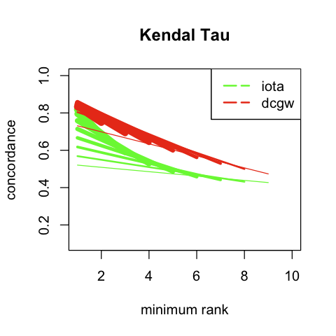
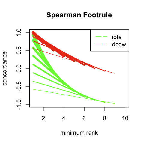
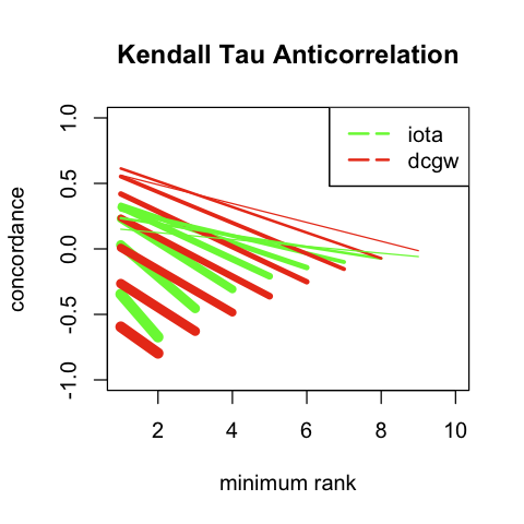
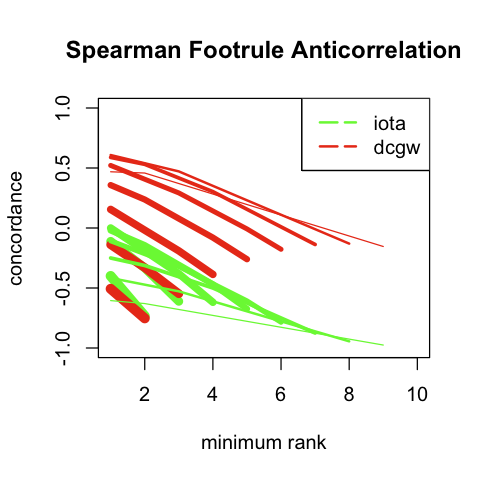
Here we choose two weighting functions that we identify as dcgw and iota. We have for every : that is, all list URLs are equally important. Instead, we have , which is inspired by the discounted cumulative gain (DCG) measure; that is, we can imagine that the tenth URL in the result list is about less important than —relatively speaking— the first one.
We created this test: we take two lists and , and we consider these lists composed of the simbols ’1’ throught ’20’ and thus with nothing in common. We start creating lists with increasing common intersection: and with one common item: , , till , then with two consecutive items , , till and eventually with 10 common consecutive items .
In Figure 2, we present the concordance measure results using Spearman’s footrule and Kendal Tau. In red, we show the list concordance measures using weights and in green without weights. The width of the lines represents the number of common items in the lists: the thinnest lines represent lists with only one item in common, the thickest 10 (one point). Consider the thinnest lines: Spearman’s footrule has the largest difference with weights and without; when the two lists have only the first item in common, the minimum rank is 1, the weighted measure is about 0.62 and the unweighted is 0.18. Both measures decreases when we choose as common element the second item towards the ninth element. The weighted measures are more sensitive for sparse lists and with high correlation in the high ranks. In Figure 2, we show the same analysis but instead of creating similar lists, we create anti-correlated similar lists. The weighted measures are less sensitive in capturing anti correlation. Even thought this is an example where the same weighting function achieves contrasting and opposite results, it shows a case where the function choice must rely on the context for which the function is applied for. In this work, we are actually interested in finding a measure that can capture both properties.
At this time, we believe that the solution must rely on a supervised method where a third party (a crowd base similarity measures) or a feed back system can be deployed to tune the weighting function knowing the context. In a different work, we prove that the weighed Spearman’s Footrule and Kendall Tau for partial lists (as described here) respect the Diaconis-Graham inequality, thus they are equivalent as discriminative power and we can choose either one (footrule because of its computational simplicity) [9].
3.3 Distribution Similarity
As in the measures for comparing sets and lists, there are many measures in the literature to compute the similarity between distributions —i.e., stochastic distances. For example, a document can be represented as a word–count histogram (which can be normalized naturally to a distribution), and this idea can be easily extended to a set of documents. Among distribution measures, we present and use here the measure from [21], which is identified in [6] as one of the best performing measures. The measure extends the well-known Kolmogorov-Smirnov measure and is defined as
| (9) |
where and are the cumulative distribution functions and and are the values for the element from these functions. This measure is symmetric and its value ranges in , where the result is zero when two input distributions are identical. In practice, we can use stochastic distances to compare the contents of search engines results.
We can also determine whether or not two documents are duplicate by using a set of these stochastic measures and use their confidence levels to flag equality/difference by a consensus based approach (see Section 5.3.1 and [6]); that is, if the measure majority suggests equivalence, we consider the document duplicates, otherwise they are not duplicate. Of course, stochastic measures will compare distributions, so we are really saying that two distributions are similar, we infer that they bring forth the same information, then we deduce that the documents can be considered duplicates or having similar contents.
Example. Consider two documents as a sequence of letters and , the histogram representation will be and , a possible cumulative distribution extension is and , thus , they are different.
4 Application of the Theory
We next detail how we applied the theory of similarity to compute the similarity between search results from different search engines. For each case, we took only (up to) the top 10 URLs. Of course, we could extend the investigation to any number of URLs; however, as almost all users pay attention to the first page only and because we do not to try to fuse the list into a single one, the results here presented are more representative than say the collection of the first 100 URLs. 222Notice that as the result list gets longer, the more the correlation measures such as footrule is less sensitive and the confidence level drops drastically artificially creating a scenario where we cannot say anything about correlation either way.
4.1 Search Results as Sets
Search results and from two search engines for the same query can be represented as either two sets of URLs or two sets of contents, which are the terms extracted from the landing pages or documents.
As sets, the rank of any URL in the original search results was ignored in the final representation. We kept a unique copy of any element in the final lists: the duplication test was done using the shingling technique [3, 15] over the landing page contents of the URLs (see § 5.3 for details). Thus for a set of URLs, the duplicate detection is used to normalized the URLs and thus the lists; this is necessary, because different search engines may use different policy for the canonical representation of a URL. As a set of contents, no URL normalization is necessary and simply the contents union of the landing pages is used instead.
We used the Jaccard ratio to compare the resulting sets. In the sequel, we use the notation and to denote the Jaccard ratio between the sets of URLs and the contents of the corresponding landing pages, respectively. We provide a detailed description of the use of the Jaccard ratio for the contents in the following Section 5.3.
4.2 Search Results as Lists
Search results and from two search engines for the same query can be represented as two lists of URLs. We kept a unique copy of each URL in the final lists (see previous section for the duplicate policy). We showed only Spearman’s footrule to compare the resulting URL sets because of the equivalence justification. In the sequel, we use the notation to denote the normalized version of Spearman’s footrule between two lists of URLs.
4.3 Search Results as Distributions
Search results and from two search engines for the same query can be represented as two distributions of term frequencies. We downloaded the landing page contents of the search result URLs. We extracted terms and their frequencies in each document. To give weight to top search results, we created distributions from the top- search results for different values of . We used the measure to compare the resulting distributions. In the sequel, we use the notation to denote the measure between two distributions of landing page contents from two sets of URLs.
5 Experimental Methodology
Using a fully automated process, we have been collecting and recording the performance of two major search engines for about two months for a total of up to 1,000 queries per day for about 20 countries (50 queries a day per country) a few may address the country as a region but as we still show in the following the terminology is completely immaterial. For brevity, we will focus on 4 representative countries in the sequel. In this section, we present how we chose our queries, how we extracted search results and their landing pages, and how we computed similarity.
5.1 Sampling Queries
Users submit a stream of queries every day. These queries are easily classified geographically based on the country of the origin where the query was submitted; for example, United States (US), Japan (JP), France (FR), and Taiwan (TW). For each country, a uniformly random query subset sample is selected out of the entire query stream daily. This original sample had one million queries a day and is used by multiple internal customers (within Yahoo!). To make the scale of our experimentation manageable, we performed another uniformly random selection of 1,000 queries (about 50 per country) out of this sample. To reduce the sampling error, we used the stratified sampling technique with three strata of highly frequent, frequent, and infrequent queries and sampled from each stratum with equal probability. So our sample set contains frequent queries as well as tail queries in equal amount; the sampling is time sensitive so that the same query is very unlikely to be chosen, day after day. Thus overall, we have a balanced set and frequent queries should not bias our results, and so the tail queries. 333Frequent queries are usually the queries where all engines do well because they get trained in time, and our results will show a consistent divergence.
So we do not classify the queries and we do not use any taxonomy or classification of the queries such as navigational, commercial. Unfortunately, most of this classifications are based on explicit human judgments (editors) or user-behavior feedback measures. These are beyond the scope of this work (unsupervised) but of course could be applied to the methodology. At the same time, we will show a comparison for representative queries that are used for relevance measures and where this classification is in place; in this scenario, we will show that our main message does not change, there is a divergence in the results-list contents but not necessarily in the quality of the user satisfaction.
Let us express one last note about query selection: similar queries, which differ very little, can be selected in this process. The fact the sampling is done during a long period of time and for different countries (different needs) and further stratified should alleviate any bias towards these similar queries. Interesting enough, out techniques can be used in practice just to find similar queries by looking at the search result lists.
5.2 Scraping Results
Each day and for each country, we repeated the following process: we submitted the queries from our daily query sample to a number of major search engines (in terms of the market share) and scraped the returned results. A query coming from France is sent to the search engines so that to reproduce the results as a French user would see from his laptop in Paris. So each engine can provide a custom experience for the same query in different markets.
For each returned URL, we downloaded the landing page contents using our production crawler. 444If we do not have it, and the site allows us crawling, we actually fetch the document. Finally, we compared the similarity between every pair of search engines using all the similarity measures discussed in § 4.
5.3 Deciding Duplicate Contents
For reasons of practicality, we performed our content-based similarity computation over shingles [3, 15] instead of raw terms. In other words, in Eq. 3, the sets and contained shingles rather than terms. We used 1,000 shingles with 10 consecutive terms per shingle. So given two items and , with the term , in the duplicate detection context, we mean where is the set of the first 1000 shingles of document and thus
Given this measure, we regarded two sets as duplicate in contents if their Jaccard ratio was above 0.5. This threshold choice is based on our previous experience with duplicate detection techniques. An intuitive suggestion about this threshold is that, when a document has more that 60% of the contents —as 10 word long sentences and considering 1000 of these— are common to another document, then the probability to have two different documents is ridiculously small especially for large documents.
Example. Consider a document as a sequence of letters and consider a window of size 3 letter (shingle). We obtain four shingles , , and . In general, if the document has words and the shingle window is of size , we have up to shingles. However, and we do not consider the multiplicity of a shingle and the document is summarized by only three shingles , and . Thus, we have . In practice, the shingles are encoded by a unique integer and we have a set of integers (letters if you will) and then we can apply the Jaccard ratio. If we take , which is the inverse of , we have four shingles but will keep only three: , and . . The two documents are not duplicate.
For deciding two documents as duplicate when using distributions, we computed their similarity using the following 10 distribution similarity measures from [6]: , , Kolmogorov-Smirnov, Kullback-Leibler, Jensen-Shannon, , Hellinger, Carmer-von Mises, Euclid, and Canberra. If more than 4 out of these 10 flagged two documents as duplicate with a statistical significance level of 5%, we considered the input documents as duplicate. So given two items and , with the term , in the duplicate detection context, we actually mean the comparison above with 10 stochastic measures and using distributions so that is a duplicate of if and only if , and as not duplicates iff (and thus ). Notice we store each measure separately and thus we can apply each measure to a single pair of documents as well as to any subset of the result list.
Example. Consider two documents as a sequence of letters and as before. These documents will have histogram and . As expected, the two documents will be considered duplicate. These measures if applied for duplicate detection are looser than the ones based on shingles: Using shingles, we may consider documents as not duplicate but they are, using distributions we may consider documents as duplicate but they are not.
5.3.1 Reduction to Spearman’s Footrule
Assume we have two lists of URLs and we want to compare their correlation. Since these lists are coming from different engines we cannot assume that the same documents have the same URL. We need to bind the document to a single URL or name and then we can perform any list based comparison. We propose to use the similarity functions in such a way to perform the unique document-URL binding. As result of this URL normalization we are able to enlarge, when possible, the Jaccard ratio of the lists and making the correlation better suited. Here we explain how we do it.
Take the two lists and , we start with and we are going to rewrite it to —i.e., the list containing only the first URL or item— and to —i.e., the empty list. We use the similarity function —shingle based comparison as in Equation 3— and —Histogram–CDF based comparison as in Equation 9. Here, we present our URL-normalization algorithm for two lists:
Normalization.
-
1.
For every and (in the order of the original list, from the highest rank to the lowest)
-
(a)
is the set .
-
(b)
is the set of duplicates we have already seen.
-
(c)
if then append the first element in that is in to
-
(d)
else append to
-
(a)
-
2.
For every and
-
(a)
is the set .
-
(b)
is the set of duplicates we have already seen.
-
(c)
if then
-
i.
append the first element in that is in to , if any (priority to the first list)
-
ii.
append the first element in that is in to , otherwise
-
i.
-
(d)
else append to
-
(a)
As a result, duplicate items are relabeled using a single name. Across different lists, this is an efficient URL normalization (independent of the search engines) and it increases the lists intersection naturally. A side effect, of this lists normalization, is that we are going to flag out duplicates within the same list (and also across lists and especially for the second list). Then, we need to penalize any search engine that introduce duplicates. We post process the lists so that any subsequent duplicate within a list will be substitute with a empty item , which will be taking the ranking position but it will not be used for any comparison. In Section 6.1 and in particular in Fig. 3, we will show that the way we perform the URL normalization across lists has very little effect and thus the little overlap it is not due to the way we perform the normalization.
Possible extension. We could use the to provide a normalizing factor for the normalized measure so that to extend the range of the measure to original interval [-1,1] and thus possibly use the footrule distribution function. This is beyond the scope of this work but a natural extension.
6 Results on Search Results Similarity
We present our observations on search results similarity in terms of the evolution of the overlap between search results as well as the correlation between overlap and quality.
6.1 Low Overlap
For a reliable data point in the past, we refer to [13]. In this reference, pairwise URL-based similarity of seven search engines over 750 URLs is computed using a version of Kendall’s tau. It shows that search engines produce quite different results except in the case of having the same third party provider of crawled contents. Another confirmation of the low overlap comes from [1] where the overlap is found to be “very small”. However, both of these studies use very few queries for supporting their findings.
Observation 1
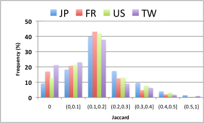
For more than 80% of the queries, the overlap between two sets of search results is less than 30%.
To support this finding, we present Fig. 3, where a histogram for the overlap in URLs is given for four representative markets. The x-axis shows the Jaccard ratio () as an interval for the URLs common to both lists and the y-axis shows the frequency of overlap.
In this figure, markets have similar behavior. The highest frequency bucket across markets is that for about 40% of the queries the overlap as measured by the Jaccard ratio fall into the interval (i.e., between 2 and 3 common URLs within top-10 results). If we add up the first three buckets, then we get what the observation claims. Over all markets, less than 5% of the queries have more than 7 common URLs.
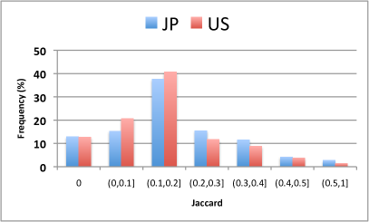
In Fig. 3, we also show that the low overlap is independent of the duplicate detection measure used from a stricter (on the left) to a looser (on the right). Notice that we performed in parallel for JP and US the same process (of course with queries chosen randomly and independently as described in Section 5.1) only using a different duplicate detection. We chose JP and US because in this example we have the largest overlap. This shows that the little overlap is because of the documents in the lists instead of the way we perform the tests (inherent property of the engines results). Of course, if we do not apply any duplicate detection, the overlap will be even lower exaggerating the divergence of the result lists. Previous works show overlap only for URL-based comparisons, so we show a larger divergence with a stronger approach for the lists comparisons. Nonetheless, despite our best effort to bring forth more common URLs in the lists, the overlap is very limited and decreasing.
If we would apply list-based correlation measures on this set as in the previous works, we will find little correlation (or un-correlation for that matter) because there is little overlap not because there is a real correlation. We will come back to this in Section 6.3.
6.2 Varying Quality: quality vs. overlap
The results in this section require a quality definition and measurement. By the quality of a set of search results for a query, we mean the relevance of the search results in satisfying the information need of the user expressed by the query (e.g., see [8] for a detailed discussion on relevance).
Among the measures to quantify the relevance, Discounted Cumulative Gain (DCG) [18] seems to be the measure preferred by most search engines. For a query set , each with ranked search results, DCG is defined as
| (10) |
where is the gain for the document for the URL at rank and is the discounting factor to bias towards top ranks. Typically, where is equal to 5, 4, 3, 2, or 1 for the judgments of Perfect, Excellent, Good, Fair or Bad results, respectively. The judgments are from editors binding the query intent to the result lists and their document contents.
In this section, we used about 800 queries selected uniformly at random from user queries submitted to our search engine (some are identical queries at different times). For each query, we scraped the top 5 search results for each of the major search engines.
We define a relative measure between two search engines and as
| (11) |
where and is the DCG for with (where we leave the true identity of the search engine anonymous for obvious reasons).
Armed with these definitions and results, we can state the relationship between quality and overlap.
Observation 2
When the overlap is low between the results of two search engines, the relative quality between search engines varies widely.
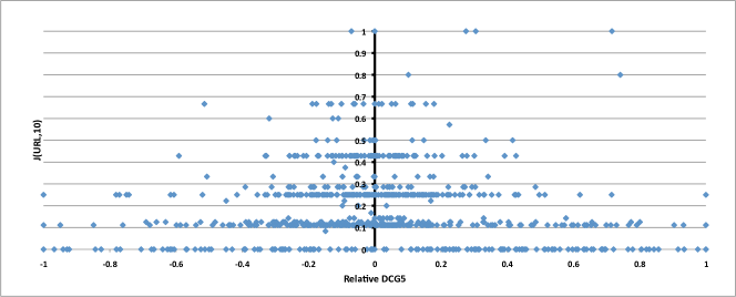
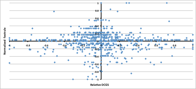
In Fig. 4, we present a comparison between the relative , (footrule) and (common intersection). There is no correlation (not upon intended) between DCG and footrule. However, we can say that when the common intersection between the result list is large enough there is no particular difference of DCG values and thus the search engines seem correlated and equivalent (i.e., having a large number of common URLs and the editors graded these URLs with similar scores based on contents and ranking, we can safely infer that the engines provide the same URLs and with the same ranking). In other words, low overlap does not necessarily mean that one of the search engines is consistently better at the search results quality.
To support this finding, we present Fig. 4, where the scatter plot between the DCG and two similarity measures is given. The x-axis shows the relative DCG measure and the y-axis shows the Jaccard ratio (top) and normalized footrule (bottom).
We have three observations: First, most of the queries have low overlap as measured by the Jaccard ratio; second, most of the queries fall into the narrow interval [-0.2, 0.2] as measured by the normalized footrule; third, for most of the queries the DCG value is orthogonal to both measures. One application of list based measures is the determination of query with little overlap to filter/reduce the list of queries that really need editorial judgments.
In Fig. 5, we provide additional evidence for our third observation (i.e., for most of the queries the DCG value is orthogonal to both measures). In this figure, we present the distribution of the over all queries such that the Jaccard ratio is less than 0.2; that is, with low overlap (1 in 5 common results). The existence of fat tails at both ends of the distribution implies a large range of values for quality as measured by the DCG (most likely the quality of the search results does not come from the common results).
6.3 Results on Similarity Measures
We conclude the experimental section by stating our last observation, which is one of the main motivations for this work.
Observation 3
Due to the low overlap between search results, content-based similarity measures provide more discriminating conclusions than URL-based similarity measures do.
We are going to break down the discussion into four parts: the relationship of content-based and URL-based Jaccard ratios (i.e., different ways of measuring overlap), URL- and content-based measures and normalized Spearman’s footrule (i.e., overlap vs. rank correlation), the effect of contents size on the similarity outcome (i.e., parameter sensitivity of content-based measures), and the relationship between content-based measures and relative DCG (i.e., overlap vs. quality).
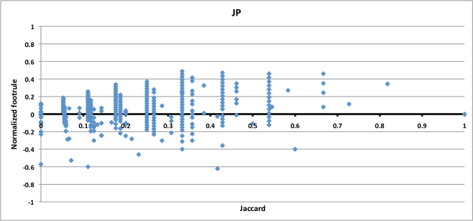
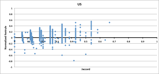
6.3.1 URL-based Jaccard ratio vs. normalized footrule
In practice, here we present how weak lists based correlation measures are and we show in a plain cross product (scatter plot) that little correlation (or lack of correlation thereof) is because the lists have really small intersection.
In Fig. 6, we show the relationship between the overlap of the URLs and the normalized footrule for two markets US and JP. As soon as the overlap of the lists decreases, the range of the normalized footrule also shrinks. Thus, at low overlap, list similarity measures will be less meaningful and less discriminating. Even the power of the URL-based Jaccard ratio decreases, helping support the need for content-based measures.
If we wanted to use Spearman’s foot rule as correlation measure we would be tempted to assume there is little correlation between the lists even in the most favorable cases. Actually, we have halved the range of the measure and thus what we really miss is the confidence in the measure more than missing a correlation measure. Thus, these measures have little or no discriminative power. List-based measure are not suitable for neither automatic nor unsupervised methods.
6.3.2 Content-based vs. URL-based Jaccard ratios
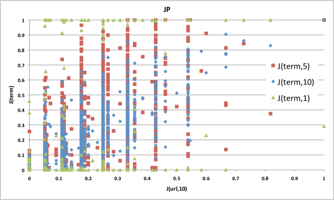
Let us refresh our memory about these contents-based measures: URL-based Jaccard ratio is computed by first normalizing the URL name by duplicate detection. Then the URL results are taken as list and the intersection/union ratio is computed. The duplicate detection is computed by using shingles or word histograms. If a threshold is reached, then the two URLs are considered identical and only one URL will be placed on both positions. For contents-based Jaccard ratio we take the shingles of all documents in a results list up to a specific rank and then we compute the intersection/union ratio of both lists. We may summarize that the former emphasizes the discrete nature of the list, instead the latter emphasizes the full contents of the documents in the lists.
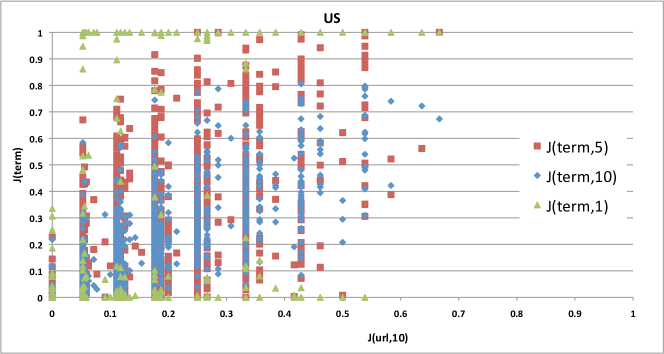
In Fig. 7, we show the relationship between the content-based Jaccard ratios for contents from top- search results for and the the URL-based Jaccard ratio for the US and JP markets. It seems that a single search result is too few to show similarity based on contents; that is, taking the top results is a hit/miss measure and thus very limited. However, if we use the first five search results we have enough information to reach the whole similarity range (i.e,. [0,1]). The ability to provide enough information in only the first five results is probably because of the emphasis of search engines to return the key results at the top.
Notice that Fig. 7 (and Fig. 6) show the same information about the URL-based Jaccard presented in Fig. 3 but we did not create bins. We want to show that even thought we wanted to collect 10 URLs per engines, there are queries for which we have less than 10. We can see that is in clusters (i.e., close vertical lines) having the same number of common URLs but different number of search results.
6.3.3 Content-based measures vs. normalized footrule
Now, we finally present the comparison between content-based measures such as and versus the most common correlation measures. The goal is to expose the different information, presented as quantitative value by the two different types of measures.
In Fig. 8, we present the relationship between the content-based measures and the normalized footrule for the US market —for which we have the largest overlap in our experiments. This is to show how small the range of the normalized footrule is and, in contrast, how the range of the content-based measure offers more variety and insights. It also shows that these effects greatly magnify when the overlap is really low, which we have shown is increasing common.
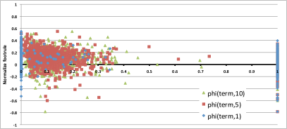
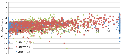
We show that the normalized footrule will be indifferent to cases where the first five documents in the lists are almost perfect duplicates ( and ). First, let us recall what means: take an engine list and consider only the first 5 URLs, take the contents of the documents as shingles (10 words each shingle without repetition) and create a set, and now perform the Jaccard ratio of the sets so determined. Let us interpret this situation: both engines give the same contents in the top of the results, it could be the same URLs (but it is not really important). On one side, this will provide the same experience to the user, we see intuitively that the engines are highly correlated for the query; on the other side, the footrule measure does not provide any information, despite our best efforts to find common items in the lists. In such a case, having a 10 URLs lists (20 total) is large enough that if only 3-4 URLs are really common and high in the result list, the footrule is dominated by the denominator and the contribution in the numerator is mixed. As a note, the size of one document, may dominate the value —even when few documents have common contents. This is a natural weight and, in practice, contents based measures emphasizes the literal size of the common documents. So we have a correlation measure for which we can interpret the value in a more intuitive fashion and it is more discriminative.
Let us take a look at the range of the measure and let us recall what the measure means: take the first 5 URLs of each lists (e.g., ), we create an histogram word–count by the contents of the documents, then we compare the histograms by creating a cumulative distribution function (CDF) and apply the formula Eq.9. If we use a lexicographical sort and a natural merge algorithm of the words, we can always create a CDF out of the histograms. We present the raw distance and the function has a natural range between 0 and 2 —where 0 means equality, 2 difference, but as a function of the number of different words the real statistically difference may be as small as 0.2). In this figure, it seems that the function has a limited range but for this function we have a significance value or p-value. There are two reasons: First, we require at a minimum 30% overlap before to perform any comparison (from histograms to CDFs); otherwise we state a distance of 1 and p-value of 1. Second, for this distance function (and for all the stochastic distance function we used in this work) we do have a statistical confidence level or p-value, which offers further granularity for the distance measure as described above. The footrule confidence will not adjust to the different range, but we have reformulated the problem in such a way that we can use a statistically sound approach with a confidence level making this measure more discriminative and suitable for a automatic approach (practically independent of the measure range).
6.3.4 Jaccard ratio with different contents sizes
In practice, we are introducing a correlation measure that return a vector of values: we can compute values of the contents-based Jaccard ratio , here we presented three values for . Here, we show how to use the vector of values to find rank correlation problems.
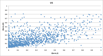
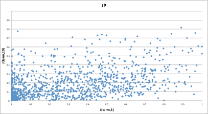
In Fig. 9, we show a scattered plot for the US and JP markets for the content-based Jaccard ratios for different contents sizes . The relatively strong correlation is evident from these plots. Intuitively, if there is a strong , that is the results lists are top heavy, having lots of common contents, this will contribute to as well.
The most interesting cases are where , that is the tail of the result lists are richer of common contents than the heads. For example, with the simple rule that and , we have found queries for which ranking of one of the search engines had problems. Let us elaborate this. If we can see two possible cases. First, the tail of the results list has contents common to the head of the other, this is the classic case of inverse correlation. Second, the tails of both lists have the common contents, thus the heads are different, this is a case of un-correlated results. In both cases, the queries exploit different engine rankings. A supervised approach may take these queries and verify whether we return the better results (editorial test) or otherwise why our system did not return the other engine results. Each such case provides a way to automatically generate training data or regression tests for machine-learned ranking systems. Think about this process of query selection as a filtering so that only the queries requiring editorial judgment are necessary and then can be used for training of ranking/relevance systems.
6.3.5 Overlap by Jaccard ratio vs. results quality by DCG
We conclude with a final evaluation of the content-based measures ( and ) with the contents quality as measured by DCG5.
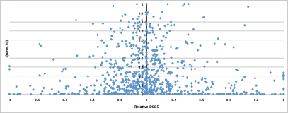
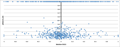
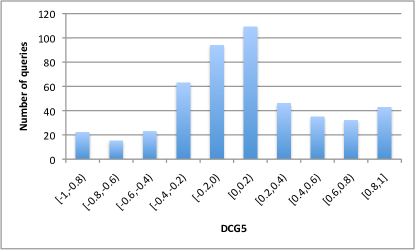
We present our experimental results in Fig. 10 and the conclusions are similar to what we have found previously and presented in Fig. 4: DCG5 varies greatly when the overlap is low (URL or contents). In other words, the results quality can cover the whole range from perfect to bad results when the overlap between the results is low. This result also justifies that low overlap between two major search engines does not necessarily make one of them also better in results quality but clearly low overlap does not mean little correlation (or inverse correlation), it means that we can infer very little about the correlation of the results.
We would like to conclude this section and the experimental result section noting that —at the least— we have presented correlation measure that are more discriminative than the existing list-based correlation measures for search engine results. These measures can be certainly used as a filtering tool so that to find the queries that really need supervised approaches or used as testing tools for the debugging of a search engine pipeline.
7 Conclusions
We present how to measure search-results overlap using URL-based and content-based measures, with contents derived from the documents at the landing pages of the URLs in search results. We extend such measures to carry weights and also work for permutations as well as partial lists. In a separate and concurrent work [9], we prove the equivalence of the weighted generalizations of two well-known list similarity measures.
We show that the overlap between the results of two major search engines is fairly low (for over 80% of the queries, no more than three URLs). This result makes the application of URL-based measures difficult, thereby increasing the importance and applicability of content-based measures. We also show that low overlap does not necessarily indicate the superiority of one search engine over another in terms of results quality; the quality can vary greatly along the quality range when the overlap is low.
We present many results on the sensitivity of the proposed measures to different parameters (e.g., number of items in the lists) as well as the relationships between the measures (list-based vs. contents-based measures). We also briefly discuss how these measures can be used to automatically create regression tests (i.e., filtering out query for which two engines do well already) or training data for machine-learned ranking systems (i.e., filtering the query that need editorial judgment). In turn, this automatic selection of queries can be used for the debugging of the search engine pipeline and automatic classification could be obtained by the engineering team.
Acknowledgments
Under the hood of this machinery, we used several components and consulted very capable engineers: Suresh Lokia for the set of queries, Kexiang Hu for the scraping tool, Marcin Kadluczka for the high level fetching system for the retrieval of the documents in real time, and Amit Sasturkar and Swapnil Hajela for the word-view pipeline and document signature. We also thank Santanu Kolay for useful discussions on various aspects of this work and Ravi Kumar for discussions on the weighted form of Kendall’s tau.
References
- [1] J. Bar-Ilan, M. Mat-Hassan, and K. Levene. Methods for comparing rankings of search engine results. Comput. Netw. ISDN Syst., 50(10):1448–1463, 2006.
- [2] K. Bharat and A. Broder. A technique for measuring the relative size and overlap of public web search engines. Comput. Netw. ISDN Syst., 30(1-7):379–388, 1998.
- [3] A. Broder. On the resemblance and containment of documents. In Proc. Compression and Complexity of Sequences (SEQUENCES), page 21. IEEE, 1997.
- [4] B. Carterette. On rank correlation and the distance between rankings. In Proc. of Conf. on Research and Dev. in Info. Retrieval (SIGIR), pages 436–443. ACM, 2009.
- [5] Moses S. Charikar. Similarity estimation techniques from rounding algorithms. In Proc. Symp. Theory of Computing (STOC), pages 380–388. ACM, 2002.
- [6] P. D’Alberto and A. Dasdan. Non-parametric information-theoretic measures of one-dimensional distribution functions from continuous time series. In Proc. Int. Conf. Data Mining (SDM), pages 685–696. SIAM, 2009.
- [7] A. Dasdan, P. D’Alberto, S. Kolay, and C. Drome. Automatic retrieval of similar content using search engine query interface. In Proc. Int. Conf. Info. and Knowledge Management (CIKM). ACM, 2009.
- [8] A. Dasdan, K. Tsioutsiouliklis, and E. Velipasaoglu. Web search engine metrics: Direct metrics to measure user satisfaction. Tutorial in the 18th Int. Conf. World Wide Web (WWW), 2009.
- [9] Ali Dasdan and Paolo D’Alberto. Weighted generalization and equivalence of Spearman’s footrule and Kendall’s tau for comparing partial and permutation rankings. Submitted for pubblication.
- [10] P. Diaconis and R. Graham. Spearman’s footrule as a measure of disarray. J. Roy. Statistics Soc., 39(Ser. B):262–268, 1977.
- [11] C. Dwork, R. Kumar, M. Naor, and D. Sivakumar. Rank aggregation methods for the web. In Proc. Int. Conf. World Wide Web (WWW), pages 613–622. ACM, 2001.
- [12] R. Fagin, R. Kumar, M. Mahdian, D. Sivakumar, and E. Vee. Comparing and aggregating rankings with ties. In Proc. Symp. Principles of Database Syst. (PODS), pages 47–58. ACM, Jun 2004.
- [13] R. Fagin, R. Kumar, and D. Sivakumar. Comparing top k lists. SIAM J. Discrete Math., 17(1):134–160, 2003.
- [14] F. Galton. Co-relations and their measurement, chiefly from anthropometric data. Proc. the Roy. Soc. of London, 45:135–145, 1888–1889.
- [15] M. R. Henzinger. Finding near-duplicate web pages: a large-scale evaluation of algorithms. In Proc. of Conf. on Research and Dev. in Info. Retrieval (SIGIR), pages 284–291. ACM, Aug 2006.
- [16] P. Jaccard. Distribution de la flore alpine dans le bassin des Dranses et dans quelques r gions voisines. Bulletin del la Soci t VauOPTdoise des Sciences Naturelles, 37:241–272, 1901.
- [17] P. Jaccard. étude comparative de la distribution florale dans une portion des Alpes et du Jura. Bulletin del la Soci t VauOPTdoise des Sciences Naturelles, 37:547–579, 1901.
- [18] K. Järvelin and J. Kekäläinen. Cumulated gain-based evaluation of IR techniques. ACM Trans. Inf. Syst., 20(4):422–446, 2002.
- [19] O. Jarvinen. Species-to-genus ratios in biogeography: A historical note. Journal of Biogeography, 9(4):363–370, Jul 1982.
- [20] M. G. Kendall. A new measure of rank correlation. Biometrika, 30(1–2):81–93, Jun. 1938.
- [21] D. Kifer, S. Ben-David, and J. Gehrke. Detecting change in data streams. In Proc. Int. Conf. Very Large Data Bases (VLDB), pages 180–191. Morgan Kaufmann, Elsevier, Aug 2004.
- [22] Ravi Kumar and Sergei Vassilvitskii. Generalized distances between rankings. In Proceedings of the 19th international conference on World wide web, WWW ’10, pages 571–580, New York, NY, USA, 2010. ACM.
- [23] K. Pearson. Notes on the history of correlation. Biometrika, 13:25–45, 1920–1921.
- [24] D. Sculley. Rank aggregation for similar items. In Proc. Int. Conf. Data Mining (SDM), 2007.
- [25] G. B. Shieh. A weighted kendall’s tau statistic. Statist. Probab. Lett., 39:17–24, 1998.
- [26] G. B. Shieh, Z. Bai, and W. Y. Tsai. Rank tests for independence - with a weighted contamination alternative. Statistica Sinica, 10:577–593, 2000.
- [27] G. L. Sievers. Weighted rank statistics for simple linear regression. J. of the American Stat. Assoc., 73(363):628–631, Sep 1978.
- [28] C. Spearman. A footrule for measuring correlation. British J of Psychology, 2:89–108, 1906.
- [29] A. Tarsitano. Nonlinear rank correlation. Working paper, 2002.
- [30] E. Yilmaz, J. A. Aslam, and S. Robertson. A new rank correlation coefficient for information retrieval. In Proc. of Conf. on Research and Dev. in Info. Retrieval (SIGIR), pages 587–594. ACM, 2008.
Reviewers’ Comments The community has spoken about and against this work. Here we share the anonymous considerations without our reply. Enjoy the drama.
Reviewers’ Comments Journal 1
Dear Paolo,
Thanks for asking. Unfortunately, after having tried quite a few potential —- reviewers, we are not able to get even one referee report. Most of them declined to review, and some of them suggest this paper is not well within the scope of —-. The guardian editors of this work have evaluated the situation, they are convinced this paper is most likely not interesting to —- readers, by looking at especially the people and journals/conferences mentioned in their related work. they consider this work is more web search than web engineering.
Therefore, it should be the best interests of the authors to find some other better suitable journal to this work. We return this paper back to you as the author, and wish you good luck somewhere else.
Regards, Wei for —- Editorial Reviewers’ Comments Journal 2
Second Round.
Dear Dr. Paolo D’Alberto:
We have received the reports from our advisors on your manuscript, "On the Divergence of Search Engines’ Results (Unsupervised Comparison of Search Engine Rankings)".
With regret, I must inform you that, based on the advice received, the Editor-in-Chief has decided that your manuscript cannot be accepted for publication in World Wide Web Journal.
Attached, please find the reviewer comments for your perusal.
I would like to thank you very much for forwarding your manuscript to us for consideration and wish you every success in finding an alternative place of publication.
Comments for the Author:
Reviewer 2: The paper addressed most of reviewers’ comment reasonably well. Presentation has been improved greatly: scoping and motivation of the problem has been substantially improved, and it’s now in a good shape. The impact of the paper remains at the same level: not as strong as groundbreaking, but a useful proof plus empirical studies on the weakness of list-based comparison methods, and also suggestion/validation of a content-based comparison method.
The reviewer recommends the paper for the publication in —-, after the minor revisions discussed below:
1) section 3.2.1
the same as they are in the original lists \sigma and \pi, respectively. –>
the same as they are in the original lists \pi and \sigma, respectively.
2) same section 3.2.1 example (a,b,c,e,f) –> (a,b,d,e,f)
3) question: why use a,b,d,e,f? why no "c"? It’s not even an issue, but just curious…
4) section 3.2.2 example (nice example, BTW) it’s not clear how (normalized version) denominator is computed in the example. has been shown to the detail, and it’ll be nice to show the same procedure for the denominator (so that the reader doesn’t have to wonder.) Also it seems that uses rather than at the top, so shouldn’t it be , instead of ? Also, ’s can be cancelled form the top and bottom, so two ’s should cancel each other?
5) Figure 1. For the same countries, "JP" and "US", it’ll be nice to use the same color.
Reviewer 3: My primary complaints on the earlier draft were that
(1) The set (or list) similarity section is marginally related to the experimental part of the paper. (2) The contribution and the conclusion of experimental section were not clear. (3) The paper is difficult to follow at various places and needs significant revision.
In their reply, the authors tried to make the case for the relevance of their similarity part, but I am still not convinced. There are no new insights or results that the authors added to the new draft of the experiment section. The writing of the paper has improved but it still needs to be polished more. Based on these, I recommend rejecting the paper.
Here are more detailed comments.
(1) The authors argue that the similarity-metric equivalence result is significant because it gives credibility to their results in the experiment section. I do not agree with this argument. What is new in the paper (in terms of the similarity metric equivalence) is their extension of the equivalence theorem to weighted metrics. The equivalence of unweighted metrics are already known in the literature. Unfortunately, in their experimental section, the authors eventually decide that they will use only unweighted metrics. Then what was really the point of Section 3? Why do you need to prove the equivalence of weighted metrics when you do not use them?
(2) In the original review, I complained about the significance of results reported in the experimental section and the difficulty of reading parts of the section. The writing quality of the experimental section has improved in the new draft, but no new results or insights have been added. I am still not clear about what is the takeaway message of the results reported in the experimental section.
(3) At many places, the paper still needs quite a bit of proof reading and/or polishing. I will point out problems in Sec 3.2 as an example:
(a) Line 42 of Sec 3.2.1: pi(i) = n + sigma(i) - 1: what is n here? Since we are dealing with partial list, the meaning of n is different from earlier definition of n. I also believe that the equation should not have -1 at the end. Assuming n is the length of pi, when we append an element at the end of pi, its rank starts with n+1, not n.
(b) Line 58-61 of Sec 3.2.1: I do not understand this statement.
(c) Equation (5). the denominator has (n-i+1). Again, I am not clear what n means here.
(d) equation on s_w after Equation (6). I am not sure why it simplfies
to 1 - w 1/3. I also do not see why the denominator grows as .
(e) Equation (7). sigma = iota(?). Iota has not been defined.
(f) Line 31 on the right column of 5. What is F metric?
The paper has errors like these in other parts as well, which make it difficult to follow.
Reviewer 4: Second review of "On the divergence of search engines’ results" The results of Section 3 seem to be unrelated to those in later sections. There is some improvement in presentation, but further improvement is needed. Some examples: p.4 first example, sigma prime "c" replaced by "d"? How does the normalized Kw become negative? p.6 Example phi(Fsigma, Fpi) =2. The two distributions are not that different. Why the maximum difference? p.8 an example in Section 5.3.1 would help.
Sections 6.3.2- 6.3.4 need to be presented better. The figures are hard to read with three figures superimposed together. Better explanations should be provided.
First Round.
Dear Dr. Paolo D’Alberto:
We have received the reports from our advisors on your manuscript, "On the Divergence of Search Engines’ Results (Unsupervised Comparison of Search Engine Rankings)", which you submitted to World Wide Web Journal.
Based on the advice received, the Editor feels that your manuscript could be reconsidered for publication should you be prepared to incorporate major revisions. When preparing your revised manuscript, you are asked to carefully consider the reviewer comments which are attached, and submit a list of responses to the comments. Your list of responses should be uploaded as a file in addition to your revised manuscript.
COMMENTS FOR THE AUTHOR:
Reviewer 1: The paper proposes a method for comparing the results from different search engines. The paper is well motivated and has a potential of practical use. However, the first contribution claimed, proof of equivalence between a weighted generalizations of Spearman’s footrule and Kendall’s tau, is weak since it is a simple extension of the existing work, the proof for the unweighted permutations [9]. Moreover, I’m not sure whether the proof should be included in this paper. It consumes much space but it is not essential part of the paper. It would be enough to choose one of two measures. The other contributions claimed are applications of the existing work. It is difficult to find significant technical contributions.
Reviewer 2: The authors claim three main contributions - i) proof for equivalence of extended version of Spearman’s footrule and Kendall’s tau, ii) observation of divergent results from multiple search engines, and iii) content-based similarity measurement of search engine results.
First contribution appears to be a solid and useful contribution that can be used for general similarity measurement methods. However, to the reviewer, it seems that the rest of the paper is not very strongly motivated - why should readers care about the divergence of search engines? The current status of art provides a reasonable quality, and the fact that different search engines produce different results is hardly surprising considering the scale of web and the difficulty of search task. The paper may be interesting for some engineers at Google, Yahoo, or Microsoft, but to the general audience, it’s not clear what they gain from the paper. Authors recommend that users should use meta-search or multiple search engines because of the divergence, but it seems that users are fine with what they get from a single search engine, and the suggestion doesn’t seem to make sense.
One possible direction for improvement is to discuss more about the detailed anlysis of search engine biases, such as which search engine is good at what, and not so good at what, rather than simply reporting that they are different. This may give general audiences a better insight toward the current status of multiple search engine technologies.
Reviewer 3: Summary:
In this paper the authors present URL-based and content-based measures of search engine result overlap. For URLs, they show that (1) even with normalized URLs, overlap (e.g. Jaccard ratio) is generally small, and (2) URL overlap is not indicative of quality. Given this, they suggest content-based approaches for measuring overlap. They show content-based approaches (e.g. shingle overlap from the top n pages) provides a wider range of values, and again no correlation between overlap and quality. These apply to both ordered (set) and unordered (list) measures. These measures can be used, for example, to see where one search engine performs better than another.
Comments:
* The bulk of the contributions seems to be Section 3 and small observations about the figures throughout Section 6. Could use more insight into what each of the graphs really means. Isn’t the "second" contribution really just motivation for the use of content-based comparisons?
* Very long discussion and proofs of footrule and Kendall’s, their equivalence, etc in Section 3… but then the figures seem to suggest footrule is not particularly useful for comparing search results anyways (due to high divergence)? So then why is their equivalence or the extension to weighted lists important here?
* A lot of the details of the paper seem to be in areas mostly unrelated to what I perceived as the main point (most of Section 3, 5.1, 5.3).
* Query classification (e.g. navigational) could make a huge difference on the results. One would reasonably expect navigational queries to have much higher URL correlation than, say, informational queries, particularly in the top few results. The high J(term,1) and phi(term,1) results in Fig 4 and 6 could be due to this, and it could raise the overall content-based similarity scores.
* The paper could benefit from reorganization. Motivations aren’t as clear upfront (e.g. at the time, I didn’t really know why I was reading through the messy details of Section 3). The "Normalization" steps in Section 5.3.1 is almost unreadable. I’m not clear what this is saying or what each of the symbols really means.
* Are the x-y labels for Fig 7 (JP) correct?
Reviewer 4: The paper has three results. (1) a proof that Spearman’s footrule and Kendall’ tau are equivalent. (2) Most queries have very little overlap for the top two search engines, Google and Yahoo, in their top 10 results. (3) Introduce measures to compare performance of search engines based on contents. The results are somewhat interesting, but the presentation needs improvement. There is not even a single example in the entire paper. The authors should utilize examples to illustrate their ideas.
Specifice comments:
p.5 Give the intuitive idea of Kw in equation (6). line after equation (8) Should it be the numerator instead of the denominator? SMetric space: Should F be Section 3.2.4 Equivalence usually implies "stronger than within small constant multiples of one another"?
p.7 Section 4.4 second para What is exactly the similarity score defined in [22]?
p.8 left line 32 Should the Jaccard ratio be above 0.5? Section 5.3.1 I am lost. What is sigma zero? What is the intuition for normalization. Please explain Step 1 and step 2 clearly.
p.9 right l.48 Why are "the search engines seem correlated"?
p.10 first para Fig. 3 The values in the range [0.4, 1] seem to be larger than those in [-0.4, -1]. Does’nt that imply one search engine has better performance than the other?
p.10 I don’t understand what Fig. 4 shows. Please explain clearly. What exactly are the purposes for detecting near-duplicates using shingles? Is it used to detect near duplicates among documents in the search result of one search engine and those in the search result of the other? Or, the near duplicates are detected among documents within single search engine?
p.11 left lines 31-33 I have difficulty understanding this sentence. l.57 What is meant by "we could create queries for which ranking pf one of the search engines had problems" and how? Section 6.3.5 For the statement "DCG5 varies greatly when the overlap is low", should’nt DCG5 be the Y-axis and the overlap be the X-axis? Conclusion It is not clear "how these measures can be used to atomatically create regression tests or training data for machine-learned ranking systems"?
Reviewers’ Comments Conference 1 to add