Semiclassical Wigner distribution for two-mode entangled state
generated by an optical parametric oscillator

Abstract

We derive the steady state solution of the Fokker-Planck equation that describes the dynamics of the nondegenerate optical parametric oscillator in the truncated Wigner representation of the density operator. We assume that the pump mode is strongly damped, which permits its adiabatic elimination. When the elimination is correctly executed, the resulting stochastic equations contain multiplicative noise terms, and do not admit a potential solution. However, we develop an heuristic scheme leading to a satisfactory steady-state solution. This provides a clear view of the intracavity two-mode entangled state valid in all operating regimes of the OPO. A nongaussian distribution is obtained for the above threshold solution.

I Introduction

Among the quasiprobability functions that represent the density operator of a quantum state, the Wigner distribution has undoubtedly advantages over others, since in this phase space representation the quantum-classical correspondence is, in general, much more visible. At the same time these functions contain all information available in the density operator.

Unfortunately, just a few states have been represented by this distribution due to the difficulty to solve Fokker-Planck equations for nonlinear systems. Indeed, the phase space description of quantum systems is well known for quadratic hamiltonians carmichael ; dodonov , but very little is known for nonlinear systems, such as, for example, the single-mode degenerate parametric oscillator kinsler , or the transverse multimode degenerate parametric oscillator kaled2 .

Of special interest is the two-mode entangled state generated in the optical parametric oscillator (OPO) villar2 , used in many experiments of quantum information and recently shown to produce tripartite continuous variable entanglement science-usp . The Wigner distribution of this state was obtained exactly using the solution derived from the complex P-representation (after adiabatic elimination of the pump mode) karen , and tranformed into a Wigner distribution. Since this analytical result appears as an infinite series of gamma functions (hypergeometric series), some important physical aspects are hidden by its mathematical complexity. For example, two-mode entanglement is not of easy identification from the usual partial transpose criterion simon ; duan . The same happens to the generalized P-representation for the intracavity parametric oscillator derived in Ref. mcneil . In order to calculate the intensity correlations, the authors obtained an integral expression that depends on degenerate hypergeometric functions, and the outcome also depends on an infinite sum.

In the present work, we derive the Wigner function of a two-mode quantum state of the electromagnetic field generated by an OPO using a truncated Wigner equation. This truncated approximation is valid when the nonlinearity is small enough, which is true for most of the OPO experiments developed so far. A simple expression is obtained for the Wigner distribution, which renders clear the many quantum features of the intracavity OPO field such as squeezing and entanglement. Moreover, this expression is valid in all regions of the OPO operation regimes, that is, below, and above threshold, where the validity of both the linear approximation, and the perturbation theory break down. This distribution also describes the OPO quantum fluctuations properly around the operation threshold, while the usual linear approach provides divergent results. In order to illustrate the reliability of the distribution we obtain, we compare moments calculated with this Wigner function with those obtained by numerical simulations using the positive P-representation of the density operator without any approximations, that is, full quantum result for any control parameters of the OPO.

The paper is organized as follows. Section II presents the master equation describing the three-mode OPO dynamics in the Wigner representation. The correct adiabatic elimination of the pump mode is addressed in Sec. III, where we show that the standard procedure graham leads to wrong results for some quadrature moments. After truncation and adiabatic elimination a two-mode Fokker-Planck is obtained which does not satisfy the conditions for a steady-state potential solution. However, we show that an approximately potential solution can be found which reproduces satisfactorily many quantum features of the OPO (Sec. IV). Comparisons with the linear theory are exhibited in Sec. V. Section VI contains the concluding remarks.

II Theoretical model

We present here a model of three quantized modes coupled by a nonlinear crystal inside a triply resonant Fabry-Perot cavity. The Heisenberg picture Hamiltonian that describes this open system is given by carmichael

$$\hat{H} = \sum_{i=0}^{2}\hbar\omega_{i}\hat{a}_{i}^{\dagger}\hat{a}_{i}+i\hbar\chi\left(\hat{a}_{1}^{\dagger}\hat{a}_{2}^{\dagger}\hat{a}_{0}-\hat{a}_{1}\hat{a}_{2}\hat{a}_{0}^{\dagger}\right)$$ (1)

$$+ i\hbar\left(Ee^{-i\omega_{0}t}\hat{a}_{0}^{\dagger}-E^{*}e^{i\omega_{0}t}\hat{a}_{0}\right)$$

$$+ \sum_{i=0}^{2}\left(\hat{a}_{i}\hat{\Gamma}_{i}^{\dagger}+\hat{a}_{i}^{\dagger}\hat{\Gamma}_{i}\right)\;.$$

Here $E$ represents the external coherent driving pump field at frequency $\omega_{0}$. The operators $\hat{a}_{0}$, $\hat{a}_{1}$ and $\hat{a}_{2}$ represent the pump, signal and idler fields, respectively, satisfying the following frequency matching condition, $\omega_{0}=\omega_{1}+\omega_{2}$. The terms $\hat{\Gamma}_{i}$ represent damping reservoir operators, and $\chi$ is the nonlinear coupling constant due to the second order polarizability of the nonlinear crystal.

The master equation for the reduced density operator, after the elimination of the heat bath by standard techniques carmichael , is given by

$$\frac{\partial\hat{\rho}}{\partial t} = -i\sum_{i=0}^{2}\omega_{i}\left[\hat{a}_{i}^{\dagger}\hat{a}_{i},\hat{\rho}\right]+\chi\left[\hat{a}_{1}^{\dagger}\hat{a}_{2}^{\dagger}\hat{a}_{0},\hat{\rho}\right]-\chi\left[\hat{a}_{1}\hat{a}_{2}\hat{a}_{0}^{\dagger},\hat{\rho}\right]$$ (2)

$$+Ee^{-i\omega_{0}t}\left[\hat{a}_{0}^{\dagger},\hat{\rho}\right]-E^{*}e^{i\omega_{0}t}\left[\hat{a}_{0},\hat{\rho}\right]$$

$$+\sum_{i=0}^{2}\gamma_{i}\left(2\hat{a}_{i}\hat{\rho}\hat{a}_{i}^{\dagger}-\hat{a}_{i}^{\dagger}\hat{a}_{i}\hat{\rho}-\hat{\rho}\hat{a}_{i}^{\dagger}\hat{a}_{i}\right)\;,$$

where $\gamma_{i}$ is the corresponding mode damping rate.

In order to treat the operators evolution, we now turn to the method of operator representation theory. These techniques can be used to transform the density matrix equation of motion into c-number Fokker-Planck or stochastic equations. The phase space Wigner equation for the nondegenerate parametric amplifier that corresponds to the master equation (2) is then

$$\frac{\partial W}{\partial t} = \left\{\frac{\partial}{\partial\alpha_{0}}\left(i\omega_{0}\alpha_{0}+\gamma_{0}\alpha_{0}+\chi\alpha_{1}\alpha_{2}-Ee^{-i\omega_{0}t}\right)\right.$$ (3)

$$+ \frac{\partial}{\partial\alpha_{0}^{*}}\left(-i\omega_{0}\alpha_{0}^{*}+\gamma_{0}\alpha_{0}^{*}+\chi\alpha_{1}^{*}\alpha_{2}^{*}-E^{*}e^{i\omega_{0}t}\right)$$

$$+ \frac{\partial}{\partial\alpha_{1}}\left(i\omega_{1}\alpha_{1}+\gamma_{1}\alpha_{1}-\chi\alpha_{2}^{*}\alpha_{0}\right)$$

$$+ \frac{\partial}{\partial\alpha_{1}^{*}}\left(-i\omega_{1}\alpha_{1}^{*}+\gamma_{1}\alpha_{1}^{*}-\chi\alpha_{2}\alpha_{0}^{*}\right)$$

$$+ \frac{\partial}{\partial\alpha_{2}}\left(i\omega_{2}\alpha_{2}+\gamma_{2}\alpha_{2}-\chi\alpha_{1}^{*}\alpha_{0}\right)$$

$$+ \frac{\partial}{\partial\alpha_{2}^{*}}\left(-i\omega_{2}\alpha_{2}^{*}+\gamma_{2}\alpha_{2}^{*}-\chi\alpha_{1}\alpha_{0}^{*}\right)$$

$$+ \gamma_{0}\frac{\partial^{2}}{\partial\alpha_{0}\partial\alpha_{0}^{*}}+\gamma_{1}\frac{\partial^{2}}{\partial\alpha_{1}\partial\alpha_{1}^{*}}+\gamma_{2}\frac{\partial^{2}}{\partial\alpha_{2}\partial\alpha_{2}^{*}}$$

$$+ \left.\frac{\chi}{4}\left(\frac{\partial^{3}}{\partial\alpha_{1}\partial\alpha_{2}\partial\alpha_{0}^{*}}+\frac{\partial^{3}}{\partial\alpha_{1}^{*}\partial\alpha_{2}^{*}\partial\alpha_{0}}\right)\right\}W\;.$$

This is not a Fokker-Planck equation due to the third order derivative term, but in the case where $\chi$ is small enough we can drop this term, as discussed in appendix A (see Ref. polvo for a recent review of the truncated Wigner approximation and its applications). The truncated equation so obtained is a genuine Fokker-Planck equation with a positive diffusion term, and we can easily derive the corresponding stochastic differential equations in the rotating frame ($\tilde{\alpha}_{j}=\alpha_{j}\exp{(-i\omega_{j}t)}$ with $j=0,1,2$):

$$\frac{d\tilde{\alpha}_{0}}{dt}=-\gamma_{0}\tilde{\alpha}_{0}+E-\chi\tilde{\alpha}_{1}\tilde{\alpha}_{2}+\sqrt{\gamma_{0}}\xi_{0}(t)\;,$$

$$\frac{d\tilde{\alpha}_{1}}{dt}=-\gamma_{1}\tilde{\alpha}_{0}+\chi\tilde{\alpha}_{0}\tilde{\alpha}_{2}^{*}+\sqrt{\gamma_{1}}\xi_{1}(t)\;,$$

$$\frac{d\tilde{\alpha}_{2}}{dt}=-\gamma_{2}\tilde{\alpha}_{0}+\chi\tilde{\alpha}_{0}\tilde{\alpha}_{1}^{*}+\sqrt{\gamma_{2}}\xi_{2}(t)\;.$$ (4)

III Validity of the adiabatic approximation

It is possible to find a stationary solution of the truncated Fokker-Planck equation when we adiabatically eliminate the pump mode variables. This means that we are considering the relaxation rate of this mode much larger than those of the downconverted modes, that is $\gamma_{0}\gg\gamma_{1},\gamma_{2}$. The stationary solution for the pumped mode is

$$\tilde{\alpha}_{0}=\frac{1}{\gamma_{0}}\left[E-\chi\tilde{\alpha}_{1}\tilde{\alpha}_{2}+\sqrt{\gamma_{0}}\xi_{0}(t)\right]\;,$$ (5)

where the noise term is retained in the adiabatic elimination in order to properly deal with the noise dynamics. We are then left with two nonlinear dynamical equations for the complex amplitudes of the down-converted fields, where the pump amplitude is replaced by expression (5).

We now define the following real quadrature variables:

$$x_{1}=\tilde{\alpha}_{1}+\tilde{\alpha}_{1}^{*}\;,\,\,\,\,\,\,\,\,\,\,y_{1}=-i\left(\tilde{\alpha}_{1}-\tilde{\alpha}_{1}^{*}\right)\;,$$

$$x_{2}=\tilde{\alpha}_{2}+\tilde{\alpha}_{2}^{*}\;,\,\,\,\,\,\,\,\,\,\,y_{2}=-i\left(\tilde{\alpha}_{2}-\tilde{\alpha}_{2}^{*}\right)\;,$$ (6)

so that the remaining dynamical equations can be cast in the compact form:

$$\frac{d\mathbf{X}}{dt}=\mathbf{A}+\mathbf{B}\,\mathbf{\xi}(t)\;,$$ (7)

where $\mathbf{X}=[x_{1},y_{1},x_{2},y_{2}]^{T}$ is a column vector, and the drift vector is defined as

$$\mathbf{A}=\gamma\left[\begin{array}[]{c}-x_{1}+\mu x_{2}-\frac{g^{2}}{2}x_{1}\left(x_{2}^{2}+y_{2}^{2}\right)\\ \vskip 6.0pt plus 2.0pt minus 2.0pt\cr-y_{1}-\mu y_{2}-\frac{g^{2}}{2}y_{1}\left(x_{2}^{2}+y_{2}^{2}\right)\\ \vskip 6.0pt plus 2.0pt minus 2.0pt\cr-x_{2}+\mu x_{1}-\frac{g^{2}}{2}x_{2}\left(x_{1}^{2}+y_{1}^{2}\right)\\ -y_{2}-\mu y_{1}-\frac{g^{2}}{2}y_{2}\left(x_{1}^{2}+y_{1}^{2}\right)\\ \end{array}\right]\;.$$ (8)

We have set $\gamma_{1}=\gamma_{2}=\gamma$, which is a reasonable physical assumption for most OPO experiments, and defined the normalized pump parameter $\mu=\chi E/(\gamma\gamma_{0})$, as well as the nonlinear coupling $g=\chi/(\sqrt{2\gamma\gamma_{0}})$. $\mathbf{B}$ is a $4\times 6$ matrix defined as

$$\mathbf{B}=\sqrt{2\gamma}\left(\begin{array}[]{cccccc}1&0&0&0&\frac{g}{\sqrt{2}}x_{2}&\frac{g}{\sqrt{2}}y_{2}\\ 0&1&0&0&-\frac{g}{\sqrt{2}}y_{2}&\frac{g}{\sqrt{2}}x_{2}\\ 0&0&1&0&\frac{g}{\sqrt{2}}x_{1}&\frac{g}{\sqrt{2}}y_{1}\\ 0&0&0&1&-\frac{g}{\sqrt{2}}y_{1}&\frac{g}{\sqrt{2}}x_{1}\\ \end{array}\right)$$ (9)

and ${\mathbf{\xi}}(t)$ is a six component column vector whose entries are uncorrelated real Gaussian noises associated with the noise terms for the three interacting fields.

Note that the last two columns in $\mathbf{B}$ give rise to multiplicative noise terms in the stochastic equation (7). It is important to remark that if these multiplicative noise terms are drop graham , some essential quantum features, particularly important in the above threshold regime, will be lost.

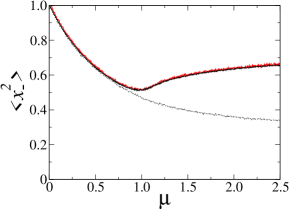
In order to illustrate the importance of the multiplicative noise terms around and above threshold, and study the validity of both the truncation and adiabatic approximations, we compare the numerical integration of the stochastic equations in the positive-P representation (without adiabatic elimination) with the stochastic equations for the truncated Wigner representation in the adiabatic approximation both with and without multiplicative noise terms. The results for the squeezed quadrature variances (defined in Sec. V) as a function of the pump level is presented in Fig. 1. The positive-P calculation clearly agrees with the truncated Wigner if the multiplicative noise terms are properly taken into account. Although valid below threshold, neglection of the multiplicative noise terms clearly fails around and above threshold, where it predicts the unphysical wallsmilburn vanishing of the intracavity quadrature noise.

Figure 1: Squeezed quadrature variance as a function of the pump level. We compare the results of the positive-P (solid black line) and truncated-Wigner stochastic equations with (solid red line) and without (dotted black line) multiplicative noise terms. The first two curves are almost indistinguishable; the third one decreases monotonically. We chose $g^{2}=0.01$ in all calculations and $\gamma_{0}=10\,\gamma$ in the positive-P simulation. All plotted quantities are dimensionless.

IV Approximate potential solution of the Fokker-Planck Equation

The set of stochastic equations (7) can be mapped onto a genuine Fokker-Planck equation:

$$\frac{\partial W(\mathbf{X})}{\partial t}=\left[-\frac{\partial}{\partial\mathbf{X}_{i}}\mathbf{A}_{i}+\frac{1}{2}\frac{\partial}{\partial\mathbf{X}_{i}}\frac{\partial}{\partial\mathbf{X}_{j}}\mathbf{D}_{ij}\right]W(\mathbf{X})$$ (10)

where the diffusion matrix is defined as $\mathbf{D}=\mathbf{B}\mathbf{B}^{T}$, and summation over repeated indices is assumed throughout the text carmichael .

Neglection of the multiplicative noise terms in the adiabatic elimination allows for a steady state solution in the potential form $W(\mathbf{X})=N\exp{(-\int\mathbf{Z}_{i}\,d\mathbf{X}_{i})}$ with $\mathbf{Z}_{i}$ given by

$$\mathbf{Z}_{i}=\mathbf{D}_{ik}^{-1}\left[2\mathbf{A}_{k}-\frac{\partial}{\partial\mathbf{X}_{j}}\mathbf{D}_{kj}\right]\;,$$ (11)

as obtained in Ref. graham . As we have seen, this distribution gives incorrect squeezing results for above threshold operation. On the other side, if multiplicative noise terms are kept, a potential solution is no longer possible

This difficulty can be circumvented if one replaces the diffusion matrix by its mean value, as explained in Appendix B, so that a potential solution for $W(\mathbf{X})$ becomes possible. This solution provides a quite simple form for the Wigner distribution which allows for the calculation of several statistical properties. We remark that this approximate potential solution is achievable only when $\gamma_{1}=\gamma_{2}\equiv\gamma$ as we have already assumed gardiner . In this case, the steady state Wigner distribution for signal and idler reads:

$$W(x_{1},y_{1},x_{2},y_{2})={\cal{N}}\exp\left\{\frac{-1}{2s(\mu)}\left[x_{1}^{2}+y_{1}^{2}+x_{2}^{2}+y_{2}^{2}\right.\right.$$

$$\left.\left.+2\mu\left(y_{1}y_{2}-x_{1}x_{2}\right)+g^{2}\left(x_{1}^{2}+y_{1}^{2}\right)\left(x_{2}^{2}+y_{2}^{2}\right)\right]\right\}$$ (12)

where ${\cal{N}}$ is the normalization constant and unimportant terms $O(g^{4})$ were neglected. We also defined

$$s(\mu)=\left\{\begin{array}[]{cc}1&(\mu\leq 1)\\ \mu&(\mu\geq 1)\\ \end{array}\right.\;.$$ (13)

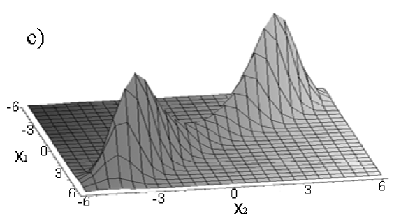
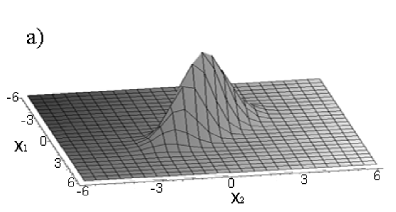
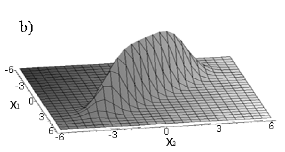
As a concrete physical example, expression (12) can describe the joint Wigner distribution for two polarization modes of a frequency degenerate type II OPO, where signal and idler are distinguished by their polarization states. All statistical properties, including experimentally accessible quantities like quadrature noise and correlations in the stationary state may be calculated with this distribution in any operation regime of the OPO within the validity of the adiabatic elimination. It is interesting to note that the distribution given by expression (12) is single peaked below threshold operation ($\mu<1$) and becomes double peaked above threshold. In Fig. 2, it is possible to visualize the conditional Wigner distribution for fixed values of $y_{1}$ and $y_{2}$, for an OPO operating below, at, and above threshold. It is easy to identify the squeezed and unsqueezed quadratures in all regimes.

Figure 2: Conditional Wigner distribution for $y_{1}=0$ and $y_{2}=0$, a) below ($\mu=0.5$); b) at ($\mu=1.0$); and c) above threshold ($\mu=1.5$). In all cases $g^{2}=0.01$. All plotted quantities are dimensionless.

For the nonlinear media employed in most OPO devices, the coupling parameter $g\ll 1$. Therefore, the first two terms in the exponent of the Wigner distribution governs the OPO behaviour below threshold. They are enough to predict the usual nonclassical features. In fact, it is evident now that the usual linearized approach to quantum noise in below-threshold OPOs is equivalent to completely neglect the $g^{2}$ term in the distribution. However, it is important to notice that for $\mu\geq 1$, the Wigner distribution becomes divergent if we neglect the $g^{2}$ term. This means that this term plays a crucial role for a complete description of the OPO behaviour at and above threshold.

Additional insight is provided by a careful investigation of the marginal distribution obtained by integrating $W(x_{1},y_{1},x_{2},y_{2})$ with respect to one mode variables. Of course, due to the symmetry of $W$, the form of the resulting marginal distribution is independent of the mode being traced out. The marginal distribution for mode 2 becomes:

$$W\left(x_{2},y_{2}\right)=\frac{2\pi{\cal{N}}\mu}{1+g^{2}\left(x_{2}^{2}+y_{2}^{2}\right)}\times$$ (14)

$$\exp\left\{\frac{-1}{2s(\mu)}\left[\left(x_{2}^{2}+y_{2}^{2}\right)\left(1-\mu^{2}\right)+g^{2}\left(x_{2}^{2}+y_{2}^{2}\right)^{2}\right]\right\}$$

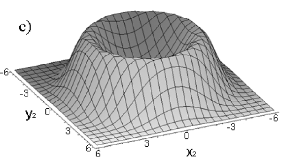
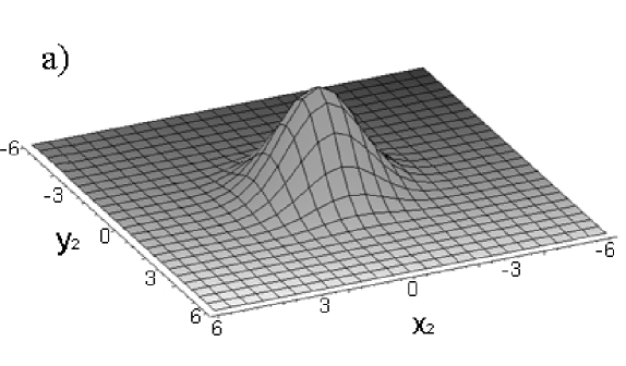
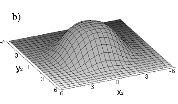
It gives the statistical properties of isolated measurements on mode 2. The variances given by this marginal distribution are larger than those of the vacuum state. This excess noise can be seen as a consequence of information loss when one looks only at part of the whole system. Fig. 3 presents the marginal distribution below, at and above threshold. Above threshold the marginal distribution is clearly peaked out of the phase space origin, what is a consequence of the macroscopic amplification of the down-converted fields. However, the distribution presents radial symmetry indicating complete phase uncertainty in each individual mode.

Figure 3: Marginal distributions: a) below threshold, $\mu=0.8$; b) at threshold, $\mu=1.0$; c) above threshold, $\mu=1.2$. In all cases $g^{2}=0.01$. All plotted quantities are dimensionless.

V Comparison with the linearized quantum approach

Almost the totality of theoretical works devoted to the analysis of quantum noise in optical systems rely on linearization of the small quantum fluctuations around the macroscopic steady state mean values. It is worth to notice that this procedure has limited validity, especially around the threshold critical point where quantum fluctuations may become comparable to the mean values. In order to evidence the breakdown of the linearized theory, we shall compare its results with those obtained from the solution of the Fokker-Planck equation (10).

The usual approach given to quantum noise in the literature is obtained from first order stochastic equations of motion ndturco ; villar . These equations are often used to predict squeezing in a linearized fluctuation analysis. They are non-classical in the sense that they can describe states without a positive Glauber-Sudarshan P-distribution, but correspond to a Gaussian Wigner distribution.

We now find it useful to introduce combined field quadratures, as in two-mode approaches used previously Caves . These combined quadratures are the Einstein-Podolsky-Rosen (EPR) variables used to characterize continuous variable entanglement between the down converted fields. They are defined as

$$x_{\pm}=\frac{x_{1}\pm x_{2}}{\sqrt{2}},\;\;\;\;\;\;y_{\pm}=\frac{y_{1}\pm y_{2}}{\sqrt{2}}.$$ (15)

These quantities correspond to the squeezed and anti-squeezed combined quadratures obtained in the linearized theory. From the first order stochastic equations one can easily obtain the steady state variances of the EPR variables ndturco ; villar :

$$\langle x_{+}^{2}\rangle = \langle y_{-}^{2}\rangle=\frac{1}{1-\mu}$$

$$\langle x_{-}^{2}\rangle = \langle y_{+}^{2}\rangle=\frac{1}{1+\mu}$$ (16)

for below threshold operation, and

$$\langle x_{+}^{2}\rangle = \langle y_{-}^{2}\rangle=\frac{1}{\mu-1}+\frac{1}{g^{2}}(\mu-1)$$

$$\langle x_{-}^{2}\rangle = \langle y_{+}^{2}\rangle=\frac{1}{2}$$ (17)

for above threshold operation.

Now let us briefly discuss the predictions of the linearized approach and its validity. The quadratures $x_{-}$ and $y_{+}$ exhibit the expected squeezing, going from the vacuum fluctuations for zero pump until 50% intracavity squeezing (which corresponds to perfect squeezing outside the cavity) at and above the oscillation threshold. The unsqueezed quadratures $x_{+}$ and $y_{-}$ present divergent behaviour around threshold, which is certainly not physical. In fact, as we shall see next, the steady state solution of the Fokker-Planck equation (10) gives a well behaved Wigner distribution which does not display any divergences. This Wigner distribution will also put limits on the amount of squeezing attainable.

In order to investigate the two-mode entanglement directly from the Wigner distribution, we now write it in terms of the EPR variables. Below threshold, where the linearization of the equation of motion is valid, we can neglect the $g^{2}$ term, and the distribution can be approximated as

$$W_{L}(x_{+},y_{+},x_{-},y_{-})={\cal{N}}exp\left\{-\frac{1}{2}\left[\left(1+\mu\right)x_{-}^{2}+\right.\right.$$

$$\left.\left.\left(1+\mu\right)y_{+}^{2}+\left(1-\mu\right)x_{+}^{2}+\left(1-\mu\right)y_{-}^{2}\right]\right\}\;.$$ (18)

With this expression we can easily calculate any moment of the distribution. For instance, we easily reobtain the results of Eqs. (16) for the intracavity noise squeezing in the combined quadratures. As we mentioned before, at threshold we have perfect external squeezing while the unsqueezed combined quadratures blow up showing the failure of linearization ndturco . Moreover, it is easy to characterize this state as entangled by using the Duan-Simon criterion simon ; duan . Above threshold we can also calculate the moments and we find that this criterion shows the sufficient condition to characterize this state as entangled, in spite of not being a Gaussian state in that regime.

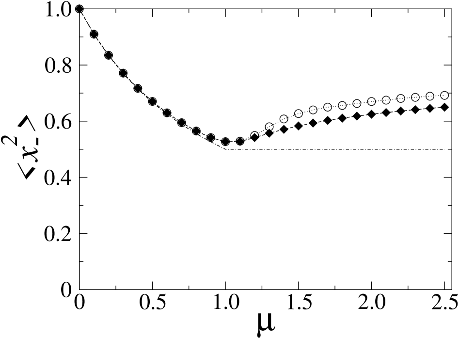
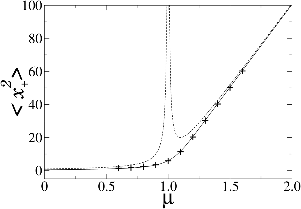
It is also interesting to compare the results obtained for $\langle x^{2}_{+}\rangle$ with the linearized theory (both below and above threshold) with those obtained from the Wigner function given by Eq. (12). This is done in Fig. (4). While the linearized approach gives a divergent behavior at the oscillation threshold, the results obtained from the truncated Wigner function gives a more realistic smooth behavior in agreement with the full quantum solution of Refs. karen ; mcneil ; singh . The results for the squeezed quadrature $\langle x^{2}_{-}\rangle$ are shown in Fig. 5 where, again, the results given by the truncated Wigner distribution agree with those obtained from the full quantum solution. Below threshold, the linearized approach also agrees with the full quantum theory and the truncated Wigner approach, but an important deviation can be observed above threshold where the linearized theory gives $\langle x^{2}_{-}\rangle=0.5$ for any pump power. The same results are obtained for the other squeezed variable $\langle y^{2}_{+}\rangle$, so that the Duan-Simon separability criterion simon ; duan shows that the two-mode quantum state is entangled. However, note that both the full quantum approach and the truncated Wigner distribution predict a less pronounced violation of the criterion above threshold.

Figure 4: Comparison between the values of the anti-squeezed variable $\langle x^{2}_{+}\rangle$ obtained from the linearized theory (dashed line) with those obtained from the Wigner function of reference karen (solid line), and the one given by Eq. (12) (crosses). In all cases we have set $g^{2}=0.01$. All plotted quantities are dimensionless.

In Refs. mcneil ; singh Fokker-Planck equations were derived for the complex-P mcneil and positive-P singh representations, and stationary solutions were obtained for the corresponding distributions. Since these Fokker-Planck equations were derived without any truncation, we can consider the stationary distributions so obtained as exact. In Ref. karen an exact stationary Wigner function was mapped from the complex-P distribution of Ref. mcneil and expressed in terms of Bessel functions. It is important to remark that the simple Wigner function presented here provides a very good approximation for those exact solutions, as can be seen in Figs. 4 and 5, even for a rather large value for the nonlinear coupling $g^{2}$.

Figure 5: Comparison between the values of the squeezed variable $\langle x^{2}_{-}\rangle$ obtained from the linearized theory (solid line) with those obtained from the Wigner function of Ref. karen (open circles), and the one given by Eq. (12) (rhombs). In all cases we set $g^{2}=0.01$. All plotted quantities are dimensionless.

VI Conclusion

By truncating the evolution equation for the Wigner function of an optical parametric oscillator, followed by the proper adiabatic elimination of the pump mode, we obtained a Fokker-Planck equation which describes satisfactorily the properties of the steady state in any operation regime of the OPO within the validity of the adiabatic elimination. This was checked by direct numerical simulation of the corresponding stochastic equations. Then we showed that the Fokker-Planck admits a simple “quasi-potential” solution. For the unsqueezed quadratures, this solution does not present the unphysical divergent behavior of the linearized theory on the oscillation threshold. Moreover, it provides good agreement with exact quasiprobabilities already available in the literature, both for the squeezed and unsqueezed quadratures. While these exact solutions are given as infinite series, the potential solution of the truncated Wigner distribution presents a simple form allowing for an easier visualization of the phase space distribution.

APPENDIX A

In order to clarify the hierarchy of the terms in the dynamical equation for the Wigner distribution, let us define the following dimensionless parameters:

• Dimensionless coupling:

  $$g\equiv\frac{\chi}{\sqrt{2\gamma\gamma_{0}}}$$ (19)

• Dimensionless pump:

  $$\mu\equiv\frac{E}{E_{c}}\equiv\frac{\chi E}{\gamma\gamma_{0}}$$ (20)

• Dimensionless time:

  $$\tau\equiv\gamma\,t$$ (21)

• Dimensionless damping:

  $$\gamma_{r}\equiv\frac{\gamma_{0}}{\gamma}$$ (22)

• Rescaled field amplitudes:

  $$\beta_{0} \equiv g\,\sqrt{2\gamma_{r}}\,\alpha_{0}\,e^{i\omega_{0}\,t}$$ (23)

  $$\beta_{1} \equiv g\,\alpha_{1}\,e^{i\omega_{1}\,t}$$ (24)

  $$\beta_{2} \equiv g\,\alpha_{2}\,e^{i\omega_{2}\,t}$$ (25)

with $\omega_{0}=\omega_{1}+\omega_{2}$ (phase match) and $E_{c}\equiv\gamma\gamma_{0}/\chi$ (threshold pump amplitude).

Perturbative approaches to the quantum stochastic equations of the parametric oscillator has been widely discussed in Refs. ndturco . In these approaches, the perturbation parameter is the dimensionless coupling $g$, usually assumed to be small as is the case in most experimental situations. The quantum fluctuations are then expanded in powers of $g$ in order to provide progressive corrections to linearized theories (the zero order terms correspond to the macroscopic mean field equations).

Therefore, let us rewrite the phase space Wigner equation for the nondegenerate parametric amplifier in terms of the rescaled amplitudes and dimensionless parameters. The equation then becomes:

$$\frac{\partial W}{\partial\tau} = \left\{\gamma_{r}\frac{\partial}{\partial\beta_{0}}\left(\beta_{0}+2\,\beta_{1}\beta_{2}-\mu\right)\right.$$

$$+ \gamma_{r}\frac{\partial}{\partial\beta_{0}^{*}}\left(\beta_{0}^{*}+2\,\beta_{1}^{*}\beta_{2}^{*}-\mu\right)$$

$$+ \frac{\partial}{\partial\beta_{1}}\left(\beta_{1}-\beta_{2}^{*}\beta_{0}\right)+\frac{\partial}{\partial\beta_{1}^{*}}\left(\beta_{1}^{*}-\beta_{2}\beta_{0}^{*}\right)$$

$$+ \frac{\partial}{\partial\beta_{2}}\left(\beta_{2}-\beta_{1}^{*}\beta_{0}\right)+\frac{\partial}{\partial\beta_{2}^{*}}\left(\beta_{2}^{*}-\beta_{1}\beta_{0}^{*}\right)$$

$$+ g^{2}\left(2\,\gamma_{r}^{2}\frac{\partial^{2}}{\partial\beta_{0}\partial\beta_{0}^{*}}+\frac{\partial^{2}}{\partial\beta_{1}\partial\beta_{1}^{*}}+\frac{\partial^{2}}{\partial\beta_{2}\partial\beta_{2}^{*}}\right)$$

$$+ \left.g^{4}\frac{\gamma_{r}}{\sqrt{2}}\left(\frac{\partial^{3}}{\partial\beta_{1}\partial\beta_{2}\partial\beta_{0}^{*}}+\frac{\partial^{3}}{\partial\beta_{1}^{*}\partial\beta_{2}^{*}\partial\beta_{0}}\right)\right\}W\;.$$

This rescaled form, evidences the hierarchy of the different terms in the dynamical Wigner equation and makes it clear that the third order derivative terms are negligible for small coupling, since it is proportional to $g^{4}$. It is interesting to make a close inspection in the physical meaning of this hierarchy. For small enough coupling ($g\ll 1$), if we neglect both the $g^{2}$ and $g^{4}$ terms, we are left with a Liouvillian evolution which is deterministic in essence, any indeterminacy comes from the initial conditions. In this case, for example, initially delta distributed amplitudes evolve as such for all times:

$$W(t)=C\,\delta(\beta_{0}-\beta_{0}(t))\,\delta(\beta_{1}-\beta_{1}(t))\,\delta(\beta_{2}-\beta_{2}(t))\;.$$ (27)

This corresponds to a classical deterministic evolution of the system.

As $g$ is continuously increased, the next approximation corresponds to neglecting only the $g^{4}$ term. In this case, Eq. (APPENDIX A) assumes the form of a standard Fokker-Planck equation, leading to the usual diffusive evolution with a possible stationary state (under self pulsing conditions, for instance, there is no stationary solution).

Finally, there are effects of the $g^{4}$ term which are essentially quantum mechanical, but have received little attention in the literature. However, these effects require a coupling constant consideraby larger than what is experimentally available in parametric systems.

APPENDIX B

Here we clarify the steady state solution derivation of the effective Fokker-Planck equation for the two down-converted modes of the field, after adiabatic elimination of the pump. We begin with the set of stochastic differential equations in the rotating frame, associated with the truncated Fokker-Planck equation for three modes

$$\frac{d\alpha_{0}}{dt}=-\gamma_{0}\alpha_{0}+E-\chi\alpha_{1}\alpha_{2}+\sqrt{\gamma_{0}}\xi_{0}(t)$$

$$\frac{d\alpha_{1}}{dt}=-\gamma_{1}\alpha_{1}+\chi\alpha_{0}\alpha_{2}^{*}+\sqrt{\gamma_{1}}\xi_{1}(t)$$

$$\frac{d\alpha_{2}}{dt}=-\gamma_{2}\alpha_{2}+\chi\alpha_{0}\alpha_{1}^{*}+\sqrt{\gamma_{2}}\xi_{2}(t)$$ (28)

The adiabatic elimination of the pump mode requires a special care. We need to keep the fluctuations in the steady state beacause they provide important additional coupling between the down-converted modes. The stationary solution of the pumped mode will be taken as

$$\alpha_{0}=\frac{1}{\gamma_{0}}\left(E-\chi\alpha_{1}\alpha_{2}+\sqrt{\gamma_{0}}\xi_{0}(t)\right)$$ (29)

We now substitute this expression into the other two amplitude mode equations to have the effective dynamical nonlinear equations,

$$\frac{d\alpha_{1}}{dt} = -\gamma_{1}\alpha_{0}+\chi\alpha_{2}^{*}\frac{1}{\gamma_{0}}\left(E-\chi\alpha_{1}\alpha_{2}+\sqrt{\gamma_{0}}\xi_{0}\right)+\sqrt{\gamma_{1}}\xi_{1}$$

$$\frac{d\alpha_{2}}{dt} = -\gamma_{2}\alpha_{0}+\chi\alpha_{1}^{*}\frac{1}{\gamma_{0}}\left(E-\chi\alpha_{1}\alpha_{2}+\sqrt{\gamma_{0}}\xi_{0}\right)+\sqrt{\gamma_{2}}\xi_{2}$$

In the vacuum state $\langle\alpha_{i}\alpha^{*}_{i}\rangle=1/2$, and $\langle\xi_{i}(t)^{*}\xi_{j}(t^{\prime})\rangle=\delta_{ij}\delta(t-t^{\prime})$. It is clear from the above equations that the pump noise enhances the coupling between the amplitudes (quadratures) of the down-converted modes.

In terms of real-quadrature variables,

$$x_{1}=\alpha_{1}+\alpha_{1}^{*}\,\,\,\,\,\,\,\,\,\,y_{1}=-i\left(\alpha_{1}+\alpha_{1}^{*}\right)$$

$$x_{2}=\alpha_{2}+\alpha_{2}^{*}\,\,\,\,\,\,\,\,\,\,y_{2}=-i\left(\alpha_{2}+\alpha_{2}^{*}\right)$$ (31)

the stochastic equations (LABEL:eq32) can be written in the form

$$\frac{d\mathbb{X}}{dt}=\mathbb{A}+\mathbb{B}\,\mathbf{\eta}(t)$$ (32)

where $\mathbb{X}$ is a vector that has the four quadratures as components, and the drift vector is defined as

$$\mathbb{A}=\gamma\left[\begin{array}[]{c}-x_{1}+\mu x_{2}-\frac{g^{2}}{2}x_{1}\left(x_{2}^{2}+y_{2}^{2}\right)\\ \vskip 6.0pt plus 2.0pt minus 2.0pt\cr-y_{1}-\mu y_{2}-\frac{g^{2}}{2}y_{1}\left(x_{2}^{2}+y_{2}^{2}\right)\\ \vskip 6.0pt plus 2.0pt minus 2.0pt\cr-x_{2}+\mu x_{1}-\frac{g^{2}}{2}x_{2}\left(x_{1}^{2}+y_{1}^{2}\right)\\ -y_{2}-\mu y_{1}-\frac{g^{2}}{2}y_{2}\left(x_{1}^{2}+y_{1}^{2}\right)\\ \end{array}\right]$$ (33)

where we have defined the adimensional pump parameter $\mu=\frac{\chi E}{\gamma\gamma_{0}}$, and the nonlinear coupling $g=\frac{\chi}{\sqrt{2\gamma\gamma_{0}}}$. $\mathbb{B}$ is a $4\times 6$ matrix defined as

$$\mathbb{B}=\sqrt{2\gamma}\left(\begin{array}[]{cccccc}1&0&0&0&\frac{g}{\sqrt{2}}x_{2}&\frac{g}{\sqrt{2}}y_{2}\\ 0&1&0&0&-\frac{g}{\sqrt{2}}y_{2}&\frac{g}{\sqrt{2}}x_{2}\\ 0&0&1&0&\frac{g}{\sqrt{2}}x_{1}&\frac{g}{\sqrt{2}}y_{1}\\ 0&0&0&1&-\frac{g}{\sqrt{2}}y_{1}&\frac{g}{\sqrt{2}}x_{1}\\ \end{array}\right)$$ (34)

and $\mathbb{\eta}(t)$ is a vector with six uncorrelated real gaussian noise components.

Associated with this set of stochastic equation there is a Fokker-Planck equation that can be written as

$$\frac{\partial P(\mathbb{X})}{\partial t}=\left[-\frac{\partial}{\partial\mathbb{X}_{i}}\mathbb{A}_{i}+\frac{1}{2}\frac{\partial}{\partial\mathbb{X}_{i}}\frac{\partial}{\partial\mathbb{X}_{j}}\mathbb{D}_{ij}\right]P(\mathbb{X})$$ (35)

where the diffusion matrix is defined as $\mathbb{D}=\mathbb{B}\mathbb{B}^{T}$ and has the following expression

$$\mathbb{D}=2\gamma\left(\begin{array}[]{cccc}a&0&c&d\\ 0&a&-d&c\\ c&-d&b&0\\ d&c&0&b\\ \end{array}\right)$$ (36)

Its inverse reads

$$\mathbb{D^{-1}}=\frac{2}{\gamma\left(ab-c^{2}-d^{2}\right)}\left(\begin{array}[]{cccc}b&0&-c&-d\\ 0&b&d&-c\\ -c&d&a&0\\ -d&-c&0&a\\ \end{array}\right)$$ (37)

where we have defined

$$a = 1+\frac{g^{2}}{2}\left(x_{2}^{2}+y_{2}^{2}\right)$$

$$b = 1+\frac{g^{2}}{2}\left(x_{1}^{2}+y_{1}^{2}\right)$$

$$c = \frac{g^{2}}{2}\left(x_{1}x_{2}+y_{1}y_{2}\right)$$

$$d = \frac{g^{2}}{2}\left(x_{1}y_{2}-y_{1}x_{2}\right)$$ (38)

and $ab-c^{2}-d^{2}=1+\frac{g^{2}}{2}\left(x_{1}^{2}+y_{1}^{2}+x_{2}^{2}+y_{2}^{2}\right)$

The Fokker-Planck equation admits a potential steady state solution in the form $P(\mathbb{X})=N\exp{-\int\sum_{i}\mathbb{Z}_{i}\mathbb{X}_{i}}$, where $\mathbb{Z}_{i}$ given by

$$\mathbb{Z}_{i}=\sum_{k}\mathbb{D}_{ik}^{-1}\left[2\mathbb{A}_{k}-\sum_{j}\frac{\partial}{\partial\mathbb{X}_{j}}\mathbb{D}_{ij}\right]$$ (39)

if the potential condition, $\,\partial_{i}\mathbb{Z}_{j}=\partial_{j}\mathbb{Z}_{i}\,$, is satisfied.

In the present case the $\mathbb{Z}$ vector is written as

$$Z_{1} = \frac{1}{1+\frac{g^{2}}{2}(x_{1}^{2}+y_{1}^{2}+x_{2}^{2}+y_{2}^{2})}\times$$

$$\left[-(1+g^{2})x_{1}+\mu x_{2}-\frac{g^{2}}{2}x_{1}\left(x_{1}^{2}+y_{1}^{2}\right)\right]$$

$$Z_{2} = \frac{1}{1+\frac{g^{2}}{2}(x_{1}^{2}+y_{1}^{2}+x_{2}^{2}+y_{2}^{2})}\times$$

$$\left[-(1+g^{2})y_{1}+\mu y_{2}-\frac{g^{2}}{2}y_{1}\left(x_{1}^{2}+y_{1}^{2}\right)\right]$$

$$Z_{3} = \frac{1}{1+\frac{g^{2}}{2}(x_{1}^{2}+y_{1}^{2}+x_{2}^{2}+y_{2}^{2})}\times$$

$$\left[-(1+g^{2})x_{2}+\mu x_{1}-\frac{g^{2}}{2}x_{2}\left(x_{2}^{2}+y_{2}^{2}\right)\right]$$

$$Z_{4} = \frac{1}{1+\frac{g^{2}}{2}(x_{1}^{2}+y_{1}^{2}+x_{2}^{2}+y_{2}^{2})}\times$$ (40)

$$\left[-(1+g^{2})y_{2}+\mu y_{1}-\frac{g^{2}}{2}y_{2}\left(x_{2}^{2}+y_{2}^{2}\right)\right]$$

Unfortunately, a potential solution cannot be achieved with the present form of matrix $\mathbb{D}$. Of course, a steady state solution of the Fokker-Planck equation still exists, since the detailed balance is established, but the solution will not be in a potential form.

For a sufficiently peaked distribution, we may approximate the diffusion matrix $\mathbb{D}$ by its average. The off diagonal terms have zero mean value due to phase space symmetry. Indeed, it is easy to verify that the dynamical equations remain unchanged under the transformation $\alpha_{1}^{\prime}=\alpha_{1}\exp(-i\theta)$ and $\alpha_{2}^{\prime}=\alpha_{2}\exp(i\theta)$. which corresponds to a definition of rotated quadratures $x_{1}^{\prime},y_{1}^{\prime},x_{2}^{\prime},y_{2}^{\prime}$. This symmetry of the dynamical equations imply in $W(x_{1},y_{1},x_{2},y_{2})=W(x_{1}^{\prime},y_{1}^{\prime},x_{2}^{\prime},y_{2}^{\prime})$ For a particular choice of $\theta=\pi/2$, this corresponds $x_{1}^{\prime}=y_{1}$, $y_{1}^{\prime}=-x_{1}$, $x_{2}^{\prime}=-y_{2}$, and $y_{2}^{\prime}=x_{2}$ so that $W(x_{1},y_{1},x_{2},y_{2})=W(y_{1},-x_{1},-y_{2},x_{2})$. This parity property of the Wigner function forces the off diagonal terms $c$ and $d$ to be zero. Note that the diagonal terms of the diffusion matrix are related to the individual intensities of the down-converted fields and can be replaced by the mean values calculated from the deterministic classical equations. This substantially simplifies the expression for vector $\mathbb{Z}$

$$Z_{1} = \frac{1}{s(\mu)}\left[-x_{1}+\mu x_{2}-\frac{g^{2}}{2}x_{1}\left(x_{2}^{2}+y_{2}^{2}\right)\right]$$

$$Z_{2} = \frac{1}{s(\mu)}\left[-y_{1}+\mu y_{2}-\frac{g^{2}}{2}y_{1}\left(x_{2}^{2}+y_{2}^{2}\right)\right]$$

$$Z_{3} = \frac{1}{s(\mu)}\left[-x_{2}+\mu x_{1}-\frac{g^{2}}{2}x_{2}\left(x_{1}^{2}+y_{1}^{2}\right)\right]$$

$$Z_{4} = \frac{1}{s(\mu)}\left[-y_{2}+\mu y_{1}-\frac{g^{2}}{2}y_{2}\left(x_{1}^{2}+y_{1}^{2}\right)\right]$$ (41)

where $s(\mu)=1+g^{2}\,\langle x_{i}^{2}+y_{i}^{2}\rangle/2$ is given by Eq. (13).

This vector represents a conservative field that generates the approximate potential solution of the effective Fokker-Planck equation.

References

• (1) H. J. Carmichael, Statistical Methods in Quantum Optics 1 (Springer, Berlin, 1999).
• (2) V. V. Dodonov, in Theory of Nonclassical States of Light, edited by V. V. Dodonov and V. I. Man’ko (Taylor and Francis, London, 2003).
• (3) P. Kinsler, and P. D. Drummond, Phys. Rev. A 43, 6194 (1991).
• (4) P. D. Drummond and K. Dechoum, Phys. Rev. Lett. 95, 083601 (2005).
• (5) A. S. Villar, L. S. Cruz, K. N. Cassemiro, M. Martinelli and P. Nussenzveig, Phys. Rev. Lett. 95, 243603 (2005).
• (6) A. S. Coelho, F. A. S. Barbosa, K. N. Cassemiro, A. S. Villar, M. Martinelli and P. Nussenzveig, Science 326, 823 (2009); A. S. Villar, M. Martinelli, C. Fabre and P. Nussenzveig, Phys. Rev. Lett. 97, 140504 (2006).
• (7) K. V. Kheruntsyan, and K. G. Petrosyan, Phys. Rev. A 62, 015801 (2000).
• (8) R. Simon, Phys. Rev. Lett. 84, 2726 (2000).
• (9) L. M. Duan, G. Giedke, J. I. Cirac, and P. Zoller, Phys. Rev. Lett. 84, 2722 (2000).
• (10) K. J. McNeil and C. W. Gardiner, Phys. Rev. A , 28, 1560 (1983).
• (11) R. Graham, Phys. Lett. A 32, 373 (1970); Statistical theory of instabilities in stationary non-equilibrium systems with applications to lasers and nonlinear optics, Springer Tracts in Modern Physics 66, 1973.
• (12) A. Polkovnikov, arXiv:0905.3384v1 [cond-mat.stat-mech].
• (13) D. Walls and G. Milburn, Quantum Optics (Springer, Berlin, 2008).
• (14) B. Coutinho dos Santos, K. Dechoum, A. Z. Khoury and L.F. da Silva, Phys. Rev. A72, 033820, (2005).
• (15) K. Dechoum, P. D. Drummond, S. Chaturvedi, and M. D. Reid, Phys. Rev. A, 70, 053807 (2004).
• (16) C. M. Caves and B. L. Schumaker, Phys. Rev. A 31, 3068 (1985); B. L. Schumaker and C. M. Caves, ibid. 31, 3093 (1985).
• (17) H. J. Kimble, Fundamental systems in quantum optics edited by J. Dalibard, J. M. Raimond and J. Zinn-Justin (1992).
• (18) A. S. Villar, K. N. Cassemiro, K. Dechoum, A. Z. Khoury, M. Martinelli, P. Nussenzveig, J. Opt. Soc. Am. B 24, 249 (2007).
• (19) C. W. Gardiner, Handbook of Stochastic Methods (Springer, Berlin, 1985).
• (20) R. Vyas, S. Singh, Phys. Rev. Lett. 74, 2208 (1995).