Abstract:

We present a determination of the parton distributions of the nucleon from a global set of hard scattering data using the NNPDF methodology at LO and NNLO in perturbative QCD, thereby generalizing to these orders the NNPDF2.1 NLO parton set. Heavy quark masses are included using the so-called FONLL method, which is benchmarked here at NNLO. We demonstrate the stability of PDFs upon inclusion of NNLO corrections, and we investigate the convergence of the perturbative expansion by comparing LO, NLO and NNLO results. We show that the momentum sum rule can be tested with increasing accuracy at LO, NLO and NNLO. We discuss the impact of NNLO corrections on collider phenomenology, specifically by comparing to recent LHC data. We present PDF determinations using a range of values of $\alpha_{s}$, $m_{c}$ and $m_{b}$. We also present PDF determinations based on various subsets of the global dataset, show that they generally lead to less accurate phenomenology, and discuss the possibility of future PDF determinations based on collider data only.

1 Introduction

In a series of previous papers [1, 2, 3, 4, 5, 6], we have presented a novel methodology for the determination of parton distributions which strives to minimize parametrization bias and ad hoc statistical assumptions by using a Monte Carlo approach with neural networks as unbiased underlying interpolating functions. The statistical consistency of this approach was confirmed in Ref. [7] by showing explicitly that it yields a probability distribution of PDFs which, upon the inclusion of new data, behaves in accordance with Bayes’ theorem. In Ref. [8] this NNPDF methodology was used to determine a set of parton distributions based on a global dataset, using NLO QCD, with inclusion of heavy quark mass effects. This PDF set, called NNPDF2.1, is arguably the most accurate NLO PDF set currently available, from every point of view: dataset, theoretical treatment, and statistical methodology. It has been made available for a variety of values of the strong coupling and of the heavy quark masses.

In this paper, we provide companion PDF sets based on the same methodology and data, but now using LO or NNLO theory: NNPDF2.1 LO and NNPDF2.1 NNLO. Both are needed for collider phenomenology: the LO parton distributions are principally for use with LO Monte Carlos, while the NNLO sets are needed for evaluation of LHC standard candle processes, some of which (such as Higgs production) are characterized by large NNLO QCD corrections and are either measured or measurable to an accuracy which may be comparable to the size of NNLO effects.

The full theoretical framework that is necessary in order to construct NNLO (and of course LO) PDFs is already available. There are however several implementation issues which must be dealt with. At LO, parton distributions can be interpreted as probability distributions, and they are therefore non-negative: to ensure this, it will be advantageous to introduce a modification of the neural network parametrization of Ref. [6] such that positivity is hard-wired. Also, it has been suggested [9, 10] that it may be useful to relax the momentum sum rule at leading order, and use a next-to-leading order form of the strong coupling in the determination of LO PDFs. All these issues will be investigated.

As we move now to NNLO, we have to address the issue of implementing higher order corrections in a numerically efficient way. In Ref. [6] we developed a method, dubbed FastKernel, for the inclusion of NLO corrections to parton evolution and to the computation of deep-inelastic (DIS) and Drell-Yan (DY) observables, without the use of $K$-factors. Here, we will use the same method for the computation of evolution and DIS to NNLO. Heavy quark mass effects will be included using the so-called FONLL method, first developed for hadronic processes in Ref. [11] and extended to DIS in Ref. [12]: the implementation of the FONLL method up to NNLO (called FONLL-C in Ref. [12]) requires the computation of some hitherto unknown Mellin transforms, and its implementation in the FastKernel framework must be benchmarked. For Drell-Yan we will rely on the NLO FastKernel implementation of Ref. [12], with NNLO corrections to it included by means of $K$-factors (note that in other global PDF fits such as Refs. [13, 14] both NLO and NNLO corrections to Drell-Yan are included using $K$-factors). This computation of the Drell-Yan process to NNLO will also be benchmarked. For the inclusive jet cross-section we will employ the threshold approximation to the NNLO corrections, since exact results are as yet unknown: these will be implemented using the FastNLO code[15].

While we will refer to our previous papers for a general introduction to the NNPDF methodology and for a detailed description of the NNPDF2.1 NLO PDF set, here we will document all the new issues that arise in the determination of LO and NNLO PDFs, specifically those mentioned above. With LO, NLO and NNLO results at our disposal, we will be able to investigate the perturbative stability of PDFs. We will thus be able to show that for PDFs in the kinematic range currently accessible the convergence of the perturbative expansion is very good: in particular NNLO PDFs are quite close to NLO ones. In particular, we will perform a study of the momentum sum rule at LO, NLO and NNLO, based on PDF determinations in which the sum rule is not imposed as a constraint and check that indeed the sum rule follows from the experimental data. We will then perform some phenomenological NNLO studies, in particular for LHC standard candles. Finally, we will discuss, in the context of the NNLO determination — which is theoretically the most accurate — the dependence of results on the value of the strong coupling and the size of the dataset, which are the main potential sources of uncertainty.

The outline of this paper is the following. In Sect. 2 we present the experimental data used in the analysis: these only differ from those used in the NNPDF2.1 NLO determination of Ref. [8] in that the inclusion of NNLO heavy quark corrections allows for looser kinematic cuts on charm structure function data. In Sect. 3 we summarize our computation of all NNLO physical observables that enter the PDF fit, and specifically discuss the NNLO heavy quark mass implementation, and the implementation of NNLO corrections to the Drell-Yan process. Mellin transforms of the NNLO heavy quark coefficient functions are given in Appendix A. In Sect. 4 we discuss modifications to the PDF parametrization and minimization which have been performed at LO and NNLO, in particular to optimize the requirement of positivity at LO, and to obtain accurate minimizations at LO and NNLO. The NNPDF2.1 LO and NNPDF2.1 NNLO sets are presented in Sect. 5 and Sect. 6 respectively, where they are also compared to other available PDF sets. In Sect. 7 we examine the convergence of the perturbative expansions for individual PDF flavours, and perform a precision determination of the momentum carried by quarks and gluons in the nucleon. The implications of NNPDF2.1 NNLO PDFs for LHC phenomenology are reviewed in Sect. 8, where, after discussing the relevant parton luminosities, we present predictions for LHC standard candles and compare them to the LHC data which are available at present. We finally turn in Sect. 9 to the issues of the dependence of results on the value of the strong coupling, and the size of the dataset, which we will study by constructing PDFs based on various subsets of data (HERA only, DIS only, collider only, DIS+Drell-Yan). Technical details on the implementation and benchmarking of DIS structure functions and NNLO PDF evolution are collected in Appendices B and C respectively.

2 Experimental data

The experimental data on which the LO and NNLO PDF sets are based are the same as those used for the NNPDF2.1 NLO set of Ref. [8] and discussed there, with some minor differences in data and kinematic cuts which we discuss here.

Experiment	Set	Ref.	$N_{\rm dat}$	$x_{\rm min}$	$x_{\rm max}$	$Q^{2}_{\rm min}$	$Q^{2}_{\rm max}$
ZEUSF2C			69 (62)
	ZEUSF2C99	[16]	21 (18)	$5\,10^{-5}$ ($1.3\,10^{-4}$)	0.02	1.8 (4)	130
	ZEUSF2C03	[17]	31 (27)	$3\,10^{-5}$ ($7\,10^{-5}$)	0.03	2.0 (4.0)	500
	ZEUSF2C08	[18]	9	$2.2\,10^{-4}$	0.032	7.0	112
	ZEUSF2C09	[19]	8	$8\,10^{-4}$	0.03	30	1000
H1F2C			47 (45)
	H1F2C01	[20]	12 (10)	$5\,10^{-5}$ ($1.3\,10^{-4}$)	$3.2\,10^{-3}$	1.5 (3.5)	60
	H1F2C09	[21]	6	$2.4\,10^{-4}$	0.025	120	400
	H1F2C10	[22]	29	$2\,10^{-4}$	0.05	5.0	2000
LO Total			3330
NLO Total			3338
NNLO Total			3357

Table 1: Charm structure function datasets included in the NNPDF2.1 NNLO analysis. All other data are the same as in the NNPDF2.1 NLO analysis, given in Table 2 of Ref. [8]. The number of data points after kinematic cuts are shown in parentheses. In the last three lines we give the total number of datapoints included in the NNPDF2.1 LO, NLO and NNLO fits.

2.1 Data sets

The NNPDF2.1 NLO dataset includes NMC [23, 24], BCDMS [25, 26] and SLAC [27] deep–inelastic scattering (DIS) fixed target data; the combined HERA-I DIS dataset [28], HERA $F_{L}$ [29] and $F_{2}^{c}$ structure function data [16, 17, 18, 19, 20, 21, 22], ZEUS HERA-II DIS cross-sections [30, 31], CHORUS [32] inclusive neutrino DIS, and NuTeV [33, 34] dimuon production data; fixed-target E605 [35] and E866 [36, 37, 38] Drell-Yan production data; CDF [39] $W$ asymmetry and CDF [40] and D0 [41] $Z$ rapidity distributions; and CDF [42] and D0 [43] Run-II one-jet inclusive cross-sections. A scatter plot of these data in the $x,Q^{2}$ plane is displayed in Fig. 1, with the values of $x$ determined using LO kinematics.

In the NNPDF2.1 LO fit, the dataset is modified in comparison to the NLO dataset in that the $F_{L}$ structure function data are removed, since this observable vanishes at LO.

In the NNPDF2.1 NNLO fit, the dataset is modified in two respects in comparison to the NLO dataset. First, the E866 data, published as $x_{F}$ distributions, have been converted into rapidity distributions, since the use of rapidity as kinematic variable makes the inclusion of NNLO corrections simpler. This was done following the procedure discussed in Ref. [44], by using the average $p_{T}$ of the lepton pair in each bin. We have verified explicitly that if this procedure is also applied at NLO, the fit results are unchanged. Second, the NMC proton data are now included as data for reduced cross-sections, rather than for structure functions. It was shown in Ref. [45] that the impact of this different treatment is almost negligible at NLO. However the use of cross-section data is in principle preferable, as they are closer to what is actually measured. In Ref. [46] it was claimed that the treatment of these data may have a significant impact on NNLO PDFs, though this claim is not supported by preliminary investigations with NNPDF2.1 NNLO [47], or with MSTW08 [49] PDFs.

Figure 1: The experimental data which enter the NNPDF2.1 PDF determination with NNLO kinematic cuts.

2.2 Kinematic cuts

All data included in the NNPDF2.1 LO, NLO and NNLO fits are subject to cuts on the invariant mass $W^{2}$ and the scale $Q^{2}$ of the DIS final state $W^{2}_{\rm min}>12.5$ GeV² and $Q^{2}>3$ GeV². In the NLO fit, the $F_{2}^{c}$ data were subject to the further cuts $Q^{2}>4$ GeV² and $Q^{2}>10$ GeV² if $x<10^{-3}$, due to the fact that in this region NNLO massive corrections are so large that a NLO approximation is not acceptable. These cuts will be removed for the NNLO fit, in which the $F_{2}^{c}$ data will only be subject to the cuts which are common to all other DIS data. The LO fit instead will use the same cuts as the NLO one. The charm structure function data included in the NNLO fit are listed in Table 1; all other data are the same as in the NLO fit, Table 2 of Ref. [8]. The total numbers of datapoints used at LO, NLO and NNLO are also given in Table 1.

3 Physical observables

As mentioned in the introduction, there are two aspects of the theoretical implementation of QCD corrections which require some discussion away from NLO: the treatment of heavy quark masses, and the fast implementation of NNLO corrections to hadronic observables and the corresponding benchmarking. The former will be discussed in Sect. 3.1, both at LO and NNLO, while the analytic expression of various hitherto unknown NNLO coefficient functions in Mellin space are listed in Appendix A; the general-mass deep-inelastic coefficient functions will then be benchmarked in Appendix B. The latter will be discussed and benchmarked in Sect. 3.2. Perturbative evolution at NNLO will be benchmarked in Appendix C. Given that for jets we will rely on the FastNLO code [15], this provides us with a full benchmarking of all NNLO expressions used.

3.1 LO and NNLO structure functions with heavy quark mass effects

We will include heavy quark masses using the FONLL method of Ref. [11], extended to DIS in Ref. [12] (see Ref. [8] for charged-current DIS expression). In the NNPDF2.1 NLO fits [8] we used the FONLL-A scheme, which combines NLO massless perturbative evolution with the $\mathcal{O}\left(\alpha_{s}\right)$ massive coefficient functions.

At LO, the massive neutral-current coefficient function vanishes, and thus, for neutral current DIS, the FONLL scheme of Ref. [12] only differs from a naive zero-mass scheme by a damping factor which suppresses dynamically generated charm contributions below threshold. The same is true for charged-current DIS when the heavy quark is the struck quark, while for contributions in which a heavy quark is produced from a struck light quark the FONLL expression simply reduces to the parton-model (${\mathcal{O}}(\alpha_{s}^{0})$) massive coefficient function.

At NNLO, it is possible to combine NNLO massless perturbative evolution with the ${\mathcal{O}}(\alpha_{s}^{2})$ massive coefficient functions: this was called the FONLL-C scheme in Ref. [12]. It is also possible to instead combine the ${\mathcal{O}}(\alpha_{s}^{2})$ massive coefficient functions with NLO massless perturbative evolution, which was called FONLL-B scheme in Ref. [12]; a comparison of FONLL-B with FONLL-A for NLO fits will be performed elsewhere.

Different schemes for the inclusion of the heavy quark mass in DIS structure functions were benchmarked in Ref. [48], with common input toy PDFs and common choices of all other settings, such as the values of the heavy quark masses. Preliminary comparisons of FONLL-C with S-ACOT-$\chi$ at NNLO [50] suggest that the two GM-VFN schemes are numerically similar.

The charm structure functions $F_{2,c}$ and $F_{L,c}$ computed in the FONLL-C scheme are shown in Fig. 2 and Fig. 3 respectively. They are compared to the NNLO determination of the structure function in which the heavy quark mass is neglected (ZM-VFN, or zero-mass variable-flavour number scheme), and to the $O(\alpha_{s}^{2})$ computation in a fixed $n_{f}=3$ scheme with charm mass (FFN). It is clear from the plots that the FONLL-C scheme interpolates smoothly between the $O\left(\alpha_{s}^{2}\right)$ massive scheme (FFN) near the heavy quark threshold, and the $O\left(\alpha_{s}^{2}\right)$ massless scheme (ZM-VFN) at large $Q^{2}$. Mass effects are much larger for the longitudinal structure function $F_{L,c}$ than for $F_{2,c}$, so there the ZM-VFN computation is completely unreliable.

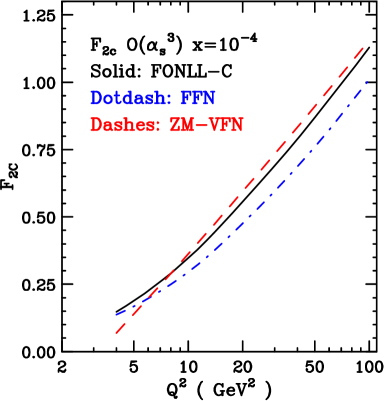
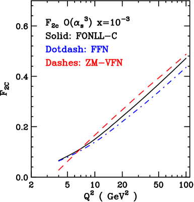
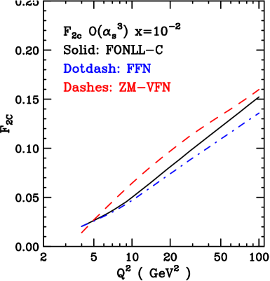
Figure 2: The charm structure function $F_{2,c}(x,Q^{2})$ as a function of $Q^{2}$ for different values of $x$ from $x=10^{-5}$ to $x=10^{-2}$ computed in the FONLL-C scheme, and compared to the zero mass (ZM-VFN) and fixed-flavour number (FFN) results. The reference input PDFs and settings of Les Houches benchmarks [48] are used throughout.

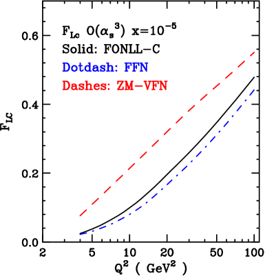
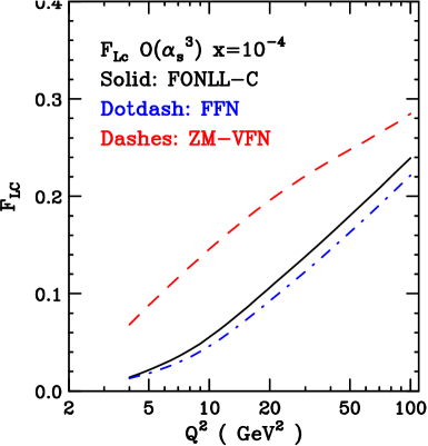
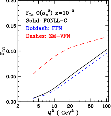
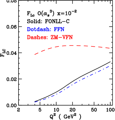
Figure 3: Same as Fig. 2 for the longitudinal charm structure function $F_{L,c}(x,Q^{2})$.

In the sequel we will adopt FONLL-C with threshold damping factor [12] as our default choice for the NNPDF2.1 NNLO fit. The heavy quark masses will also take the same default values as in the NNPDF2.1 NLO fit, namely $m_{c}=1.414$ GeV and $m_{b}=4.75$ GeV. These should be taken as pole masses, because this choice is adopted in the construction of the FONLL-B and FONLL-C expressions given in Ref. [12]. The use of running $\overline{\rm MS}$ masses has been advocated recently [51] because of the greater perturbative stability of the running mass: this possibility will be studied in future NNPDF releases.

All the above discussion applies to neutral-current structure functions. In the case of charged-current DIS, a full implementation of the FONLL-C scheme is not possible, because the massive $O(\alpha_{s}^{2})$ heavy quark coefficient functions are not available (only the asymptotic $Q^{2}\to\infty$ limit is known [52]). Consequently, in the FONLL-C charged current structure functions the $O(\alpha_{s}^{2})$ massive contribution is set to zero, while PDFs, the ZM structure functions and $\alpha_{s}$ are evaluated at NNLO. We have checked that the impact of NNLO corrections in the charged current sector is very moderate, typically well below 10%. This choice achieves the best accuracy that can be obtained from the available perturbative information without introducing any modelling.

All NNLO structure functions have been implemented in the FastKernel framework of Ref. [6]. The benchmarking of the numerical accuracy of the implementation is discussed in Appendix B.

3.2 The treatment of hadronic data

We now turn to the NNLO implementation of the hadronic data, namely, Drell-Yan, $W$ and $Z$ production, and inclusive jets.

For NNPDF2.1 NLO, Drell-Yan and vector boson production were treated consistently at NLO in perturbative QCD in all the stages of the PDF fit using the FastKernel framework [6]. The extension of the FastKernel method to NNLO is in principle straightforward, but in practice challenging, in particular because of the distribution structure and intricate choice of kinematic dependence of the NNLO coefficient functions of Ref. [53]. Therefore, here we instead adopt an approximate NNLO computation, which leads to an accuracy which is fully adequate for our purposes as we shall now show.

Figure 4: The NNLO/NLO $K$-factors for the Drell-Yan, $W$ and $Z$ production data included in the NNPDF2.1 fit.

In this approximation, Drell-Yan observables are computed with NNLO PDF evolution and NLO partonic cross-section supplemented by a $K$-factor that accounts for the missing $O(\alpha_{s}^{2})$ partonic coefficient functions. The $K$-factors are defined as the ratio of double differential cross-sections $d^{2}\sigma/dydM^{2}$ in Drell-Yan production where in the numerator we use the full NNLO expression and in the denominator the same expression but with the $\mathcal{O}\left(\alpha_{s}^{2}\right)$ correction to the partonic cross-section set to zero. In this definition the same NNLO PDFs and $\alpha_{s}$ are used both in the numerator and the denominator. This minimizes the impact of the NNLO $K$-factor corrections, which are then reduced to the missing $\mathcal{O}\left(\alpha_{s}^{2}\right)$ partonic cross-sections. These are rather small for most processes of interest, especially for collider kinematics.

Figure 5: Percentage difference between the values of the $K$ factors used in the NNPDF2.1 PDF fit (shown in Fig. 4) and their redetermination with the final NNPDF2.1 PDFs. The error bar is obtained as one sigma uncertainty over replicas.

We have computed these $K$-factors using the VRAP code [53], and cross-checked the results with the DYRAP [54] program. The $K$-factors are computed iteratively using central PDFs from a previous NNPDF2.1 NNLO fit. Results are shown in Fig. 4 for the different datasets as a function of the rapidity $y$ of the produced electroweak boson. For collider observables like $W/Z$ production at the Tevatron the $K$-factors are at the few percent level. The NNLO $K$-factors are more important for fixed-target Drell-Yan data, in particular for the E866 kinematics, where they are typically of order 10%, but sometimes as large as 25%. However, the average total experimental uncertainty on these data is larger than 20%.

The error incurred replica by replica through the use of the $K$-factor approximation is then subleading in the perturbative expansion. To see this, note that approximation in the computation of the $K$ factor comes from its dependence on the PDF. However, the $K$-factor only enters at NNLO, while the NLO is exact, so the error in the PDF used to compute the $K$-factor is $\mathcal{O}\left(\alpha_{s}^{2}\right)$. However the $K$-factor itself is $\mathcal{O}\left(\alpha_{s}^{2}\right)$, so the error in the cross section is in fact $\mathcal{O}\left(\alpha_{s}^{4}\right)$. Note that this is not the case if $K$-factors are used for both NLO and NNLO corrections (as in Refs. [13, 14]), since then the error in the PDF is $\mathcal{O}\left(\alpha_{s}\right)$, and thus $\mathcal{O}\left(\alpha_{s}^{2}\right)$ in the cross section, hence at least in principle of the same order as the NNLO correction to the cross section itself.

In Fig. 5 we show the percentage shift of the $K$-factors if they are recomputed using the final NNPDF2.1 NNLO PDF set. In order to study the possible dependence of the accuracy of the $K$-factor approximation on the choice of (central) PDF used to compute the $K$–factors, we have repeated this comparison for ten different randomly chosen replicas. The standard deviation of the results is also shown as an error bar in Fig. 5. We conclude that the accuracy is always better than 3%, which translates into an uncertainty of no more than $0.7\%$ in the cross-section.

For the inclusive jet production data exact NNLO corrections are not known. However, an approximation to the full NNLO result based on threshold resummation is available [55]. We will compute inclusive jet observables using an approximation on which PDFs are evolved at NNLO, but coefficient functions are computed using this threshold approximation of the full NNLO result, as implemented in the FastNLO code [15]. This provides us with an approximate NNLO calculation which combines the most accurate perturbative information available. Fits in which the jet data are evaluated with NLO coefficient functions, or simply removed altogether, will be discussed in Sect. 9.2.

4 Implementation issues at LO and NNLO

The parton parametrization, minimization algorithm, and determination of the optimal fit in the LO and NNLO fits presented here are the same as in the NLO PDF determination of Ref. [8], including almost all settings for the parameters which control the parametrization and minimization. The small number of changes are discussed here: first, we describe how at LO the parton parametrization is optimized in view of LO positivity constraints, and then we examine some adjustments in the choices of parameters for the genetic algorithm and the stopping of the minimization.

4.1 Parton parametrization: positivity constraints

In all previous NNPDF fits, positivity of physical observables has been imposed: beyond leading order, PDFs depend on the factorization scheme and can be either positive or negative, however cross-sections must remain non-negative [56]. Positivity of physical observables at NLO was enforced by means of Lagrange multipliers (see Ref. [8]), and the same procedure will be used here for the determination of NNLO PDFs.

However, at leading order parton distributions admit a probabilistic interpretation and are thus non-negative. The positivity constraint can then be imposed directly on all PDFs at the initial scale. Leading-order evolution preserves the probabilistic interpretation of PDFs [57, 58], hence this is sufficient to guarantee positivity at all scales. This can again be done by Lagrange multipliers, i.e. adding to the $\chi^{2}$ a large penalty term whenever any of the individual PDFs turns negative. However, in order to speed up the LO PDF fits, it is advantageous to impose positivity directly at the level of the PDF parametrization. Within the neural network PDF parametrization which we adopt, this can be done as follows. Recall that in the architecure that we adopt for neural networks, the response function is a sigmoid

$$\xi^{(l)}_{i}\,=\,g\Big{(}\sum_{j}\,\omega_{ij}^{(l)}\xi_{j}^{(l-1)}\,-\,\theta^{(l)}_{i}\Big{)},\qquad g(x)={{1}\over{1+e^{-x}}}\,,$$ (1)

for hidden layer, but it is linear in the last layer. For the LO fits, we adopt instead for the last layer a quadratic reponse function

$$\xi^{(n_{l})}_{i}\,=\,\Big{(}\sum_{j}\,\omega_{ij}^{(n_{l})}\xi_{j}^{(n_{l}-1)}\,-\,\theta^{(n_{l})}_{i}\Big{)}^{2}\,.$$ (2)

The output of the neural network, and thus the PDF, is then guaranteed to be non-negative.

The basis of PDFs that are parametrized by neural networks in NNPDF fits [4, 5] includes the gluon, quark singlet, and various other linear combinations of quark PDFs. Of these, only the gluon and singlet must be positive, since all other combinations contain differences of PDFs. However, in practice also the total valence and isospin triplet combination are positive definite. Hence the parametrization Eq. (1-2) for simplicity is adopted for all PDFs: PDFs other than singlet, gluon, valence and triplet are allowed to change sign by simply adding to the above form a constant shift. It turns out that with the constraints from the data, this is sufficient in practice to ensure positivity of all PDFs: we have checked a posteriori that for every replica the gluon and all individual quark and anti-quark flavours are positive for all values of $x$ and $Q^{2}$ for which the NNPDF2.1 LO PDFs are provided.

4.2 Minimization and stopping

	$N_{\rm gen}^{\rm wt}$	$N_{\rm gen}^{\rm mut}$	$N_{\rm gen}^{\rm max}$	$E^{\mathrm{sw}}$	$N_{\rm mut}^{a}$	$N_{\rm mut}^{b}$
LO & NLO	$10000$	2500	30000	2.6	80	10
NNLO	$10000$	2500	30000	2.3	80	30

	LO & NLO		NNLO
PDF	$N_{\rm mut}$	$\eta^{\rm k}$	$N_{\rm mut}$	$\eta^{k}$
$\Sigma(x)$	2	10,1	2	10,1
$g(x)$	2	10,1	3	10,3,0.4
$T_{3}(x)$	2	1,0.1	2	1,0.1
$V(x)$	2	1,0.1	3	8,1,0.1
$\Delta_{S}(x)$	2	1,0.1	3	5,1,0.1
$s^{+}(x)$	2	5,0.5	2	5,0.5
$s^{-}(x)$	2	1,0.1	2	1,0.1

Table 2: Parameter values for the genetic algorithm for the NNLO fits compared to those of the LO and NLO fits (top). The number of mutations and the values of the mutation rates for the individual PDFs in the NNLO fit as compared to the values of the LO and NLO fits are also given (bottom).

The poorer quality of the LO fit on the one hand, and the greater complexity of NNLO coefficient functions on the other hand, require some retuning of the parameters of the minimization algorithm.

At leading order, the best-fit value of the figure of merit $E^{(k)}$ which is being minimized for each replica (which is essentially the $\chi^{2}$ of the fit of each PDF replica to the given data replica) is on average rather larger than in an NLO fit, because of the poorer accuracy of the LO theory. This is particularly true for the Drell-Yan observables, which have large NLO corrections with a $K$-factor of order two. As a consequence, the minimum value that $E^{(k)}$ must reach for each experiment in order for the fit to stop has been increased from $E_{\rm th}=6$ to $E_{\rm th}^{\rm DY}=12$ for all Drell-Yan experiments. Furthermore, the cross-validation method that we use to determine the optimal fit stops the minimization when the moving average (over iterations of the genetic algorithm) of $E^{(k)}$ increases more than a fixed percentage threshold value $r_{v}$, larger than a typical random fluctuation. Because the size of fluctuations of $E^{(k)}$ remains fixed, while its value at best fit has increased, the typical values of $r_{v}$ are smaller at LO, and thus it turns out to be necessary to reduce the value of $r_{v}$ required for stopping to $r_{v}-1=2\cdot 10^{-4}$, from $r_{v}-1=3\cdot 10^{-4}$ used at NLO.

Even with these adjustments, for a sizable fraction of replicas the cross-validation algorithm fails to stop dynamically the minimization even after a large number of generations of the genetic algorithm. This reflects the poor accuracy of LO theory, and it could only be obviated by letting the genetic minimization run much longer. In view of the large theoretical uncertainties inherent to any LO PDF determination, as a practical compromise, we discard replicas that do not stop dynamically after 50000 iterations of the genetic algorithm, retaining only those replicas for which the stopping criterion was fulfilled. We have checked that this leads to no significant statistical bias.

At next-to-next-to-leading order the partonic cross-sections have rather more structure than at lower orders, both because of the opening of new partonic channels and because of the appearance of new transcendental functions in the perturbative results (such as higher order harmonic sums). This results in somewhat more complex PDF shapes. As a consequence, it turns out to be necessary to increase the number of mutants and mutations per PDF in the genetic minimization in order to fully explore this more complex space of minima. The NNLO settings for the genetic algorithm used for minimization are summarized in Table 2 and compared to those used at LO and NLO. The table is to be compared to Table 6 of Ref. [6] and Table 5 of Ref. [4], to which we refer for a more detailed discussion. We give the number of mutants in the two stages in which the minimization is divided, the number of mutations per PDF, and the values of the mutation rates for each PDF. We also show in a separate table the number of mutations that are applied to each PDF (which at NLO was two for all PDFs), and the values of the mutation rates $\eta^{\rm k}$ of each PDF (which at NLO were given in Ref. [4] and kept unchanged in Ref. [6]).

5 Leading order parton distributions

Parton distributions based on a leading-order QCD treatment of the data are mostly used with leading order Monte Carlo event generators, and are also of interest for comparison of QCD calculations at different perturbative orders. Of course, nothing prevents the inclusion of some NLO terms in a calculation which has LO accuracy, so in principle one could always use NLO PDFs in these and related contexts. However, in practice using NLO PDFs with LO matrix elements may lead to a poorly behaved perturbative expansion and to bad phenomenology. Indeed, the difference between the optimal PDFs determined from a LO analysis at their standard NLO counterparts is typically rather larger than NLO PDF uncertainties. Hence, the dominant uncertainty on LO PDFs is theoretical, and there is a certain latitude in their definition. Therefore, we will at first discuss various options for the construction of LO PDFs, then turn to results and comparisons, with the statistical aspects of the PDF determination now playing a relatively less important role.

PDF set	.LHgrid file	$\alpha_{s}\left(M_{Z}\right)$	Momentum SR
NNPDF2.1 LO	NNPDF21_lo_as_0119_100.LHgrid	0.119	Yes
NNPDF2.1 LO	NNPDF21_lo_as_0130_100.LHgrid	0.130	Yes
NNPDF2.1 LO*	NNPDF21_lostar_as_0119_100.LHgrid	0.119	No
NNPDF2.1 LO*	NNPDF21_lostar_as_0130_100.LHgrid	0.130	No

Table 3: Summary of NNPDF2.1 Leading Order PDF sets.

5.1 Definition of leading order PDFs

The issue of choosing the optimal parton sets to be used in combination with LO event generators has been discussed extensively. On the one hand, the possibility of using standard LO QCD theory (including the running of $\alpha_{s}$) seems theoretically simplest and most consistent. On the other hand, it could be that this leads to unacceptably poor fit quality for some datasets included in the global fit and thus modifications of the standard LO framework should be considered.

The simplest of these, advocated in [59], is to just use NLO PDFs within the LO Monte Carlo. This choice at hadron colliders can be justified by arguing that the difference between LO and NLO PDFs is driven by the difference in DIS matrix elements used in the PDF determination, but the LO and NLO matrix elements for hadron collider processes are much closer to each other, so NLO PDFs with LO collider matrix element may provide a reasonable approximation to the exact NLO result. However, it turns out that this choice requires a substantial retuning of the parameters in event generators.

An intermediate possibility consists of including some dominant NLO corrections to the LO matrix elements: for instance, in Ref. [13] it was pointed out that a sizable fraction of the large NLO and NNLO $K$ factor for Drell-Yan comes from contributions which have the same kinematics as the LO, and thus can be simply absorbed in a rescaling of the LO cross-section. The MSTW08LO PDFs of Ref. [13] where determined by rescaling the Drell-Yan cross-section in this way.

More general modifications of the standard LO were suggested in Ref. [9] and adopted in the construction of the MRST2007lomod PDFs. These PDFs are based on the observation that the LO fit quality mostly deteriorates because of the faster gluon evolution at small $x$ and the slower quark density evolution at large $x$. A possible way to improve this is to use the NLO value for the strong coupling constant together with its two-loop running. This leads to smaller values of $\alpha_{s}$ in the low $Q^{2}$ region where the small $x$ data are concentrated, and thus to slower PDF evolution. Of course, use of NLO $\alpha_{s}$ within an otherwise LO framework is a subleading and thus legitimate change. Another possibility is to relax the momentum sum rule. This alleviates another possible problem of the LO fit, namely the fact that faster small $x$ gluon evolution leads through the momentum sum rule to depletion of the gluon content at medium/large $x$, which may cause a poor description of large $x$ fixed-target data. Of course, a violation of the momentum sum rule is in principle forbidden by first principles, however it can be justified as an ad hoc phenomenological patch.

Finally, one may take the point of view [10] that the goal of LO PDFs is to be used with Monte Carlo generators, and thus they should be determined by optimizing the agreement with the data of the predictions obtained by using them in combination with a generator. This involves considering all the various modifications of the minimal LO framework discussed above, and also introducing suitable pseudodata to optimize the agreement with Monte Carlo generators. The CT09MC1/MC2 [10] PDFs were constructed in this way.

	NLO	LO $\alpha_{s}=$0.119	LO* $\alpha_{s}=$0.119	LO $\alpha_{s}=$0.130	LO* $\alpha_{s}=$0.130
Total $\chi^{2}$	1.16	1.74	1.76	1.68	1.74
$\left\langle\chi^{2\,(k)}\right\rangle$	$1.25\pm 0.07$	$1.95\pm 0.21$	$1.89\pm 0.22$	$1.95\pm 0.19$	$1.94\pm 0.18$
NMC-pd	0.97	1.43	1.13	1.18	1.12
NMC	1.72	2.05	1.68	1.74	1.72
SLAC	1.29	3.77	3.00	2.91	2.70
BCDMS	1.24	1.87	1.82	1.76	1.75
HERAI-AV	1.07	1.70	1.55	1.58	1.59
CHORUS	1.15	1.51	1.67	1.53	1.67
NTVDMN	0.45	0.69	0.71	0.71	0.78
ZEUS-H2	1.29	1.51	1.42	1.43	1.44
ZEUSF2C	0.78	1.75	1.26	1.56	1.34
H1F2C	1.51	1.77	2.00	1.81	2.02
DYE605	0.85	1.86	2.02	1.70	1.83
DYE886	1.26	1.99	2.52	2.59	3.11
CDFWASY	1.83	1.80	2.50	2.16	2.29
CDFZRAP	1.64	2.88	3.89	2.08	2.58
D0ZRAP	0.59	1.07	1.29	0.87	1.02
CDFR2KT	0.96	2.60	3.22	2.45	2.76
D0R2CON	0.83	1.18	1.56	1.17	1.35
$\left[M\right]$	1	1	$1.16\pm 0.03$	1	$1.09\pm 0.03$

Table 4: Fit quality for the global fit and for all experiments included in it for each of the NNPDF2.1 LO PDF sets. The corresponding values for the NNPDF2.1 NLO set of Ref. [60] are given for comparison. The value of the momentum integral $\left[M\right]$ Eq. (3) is also shown. All the fits have $N_{\rm rep}=100$ replicas.

5.2 Quality of the fit

We have produced four NNPDF2.1 LO PDF determinations: with two different values of $\alpha_{s}\left(M_{Z}\right)$, 0.119 and 0.130 (but always with LO running of $\alpha_{s}$), and with and without imposing the momentum sum rule. The various PDF sets, including the name of the corresponding LHAPDF grid files, are summarized in Table 3.

The $\chi^{2}$ of the four LO NNPDF2.1 sets, both for the global fit and for individual experiments, are collected in Table 4, and compared to the corresponding results of the NNPDF2.1 NLO set. The value of $\chi^{2}$ corresponds to the central PDF set (replica zero), obtained as the average over replicas, while $\langle\chi^{2\,(k)}\rangle$ is the average over the replica sample of the $\chi^{2}$ of each PDF replica. We refer to Sect. 4 of Ref. [8] for a more detailed discussion of the various statistical indicators: here it will suffice to say that all $\chi^{2}$ values are computed including the full covariance matrix of each experiment, with normalization uncertainties included using the method of Ref. [60].

The fit quality is the same within uncertainties in all four cases: the values of $\langle\chi^{2\,(k)}\rangle$ differ from each other by less than a standard deviation. The fit with a larger value $\alpha_{s}\left(M_{Z}\right)=0.130$ seems to be slightly favored, but the difference in $\chi^{2}$ as the value of $\alpha_{s}$ is varied is so small that we have not pursued further the option of also using NLO running of the strong coupling. The behaviour of the fit when the momentum sum rule (MSR) is not imposed is interesting: while the global fit quality is the same as in the fit with the MSR, the $\chi^{2}$ of individual experiments changes significantly: the fit quality improves for some sets (like for example HERA), but relaxing the MSR leads to a worse description of the hadronic data.

Note that we can fit simultaneously the Drell-Yan and deep-inelastic data without having to rescale the Drell-Yan data as discussed in Sect. 5.1 (unlike Ref. [13]). Of course, such a rescaling would likely lead to an improvement of the agreement of quality of the fit to Drell-Yan data. However, the ensuing PDFs would then be optimized for use in conjunction with codes (Monte Carlo or otherwise) in which similar corrections are also included. Optimizing LO PDFs in view of their use with some specific code such as a Monte Carlo event generator, as was done in Ref. [10], is an interesting task; however, we will not pursue it here, where we are rather mostly interested in constructing PDFs based on pure LO theory, with the clear limitations that this implies.

In Table 4 we also give the value of the momentum integral

$$\left[M\right]\equiv\int_{0}^{1}dx\,x\Sigma\left(x,Q^{2}\right)+\int_{0}^{1}dx\,xg\left(x,Q^{2}\right)\ ,$$ (3)

for each of LO PDF sets. These are determined at the starting scale $Q^{2}_{0}=2$ GeV², but note that the momentum integral $\left[M\right]$ does not depend on scale. A discussion of the behaviour of the momentum integral at LO, NLO and NNLO will be given in Sect. 7.2 below.

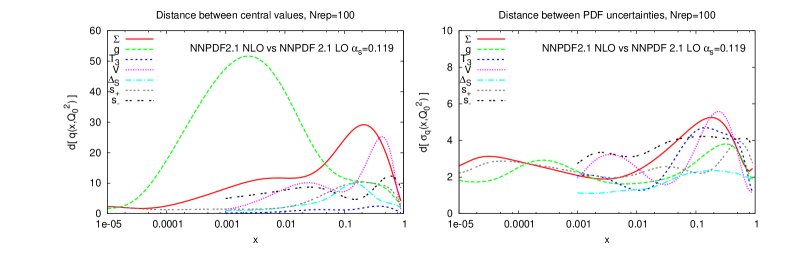
Figure 6: Distances between the reference LO and NLO NNPDF2.1 sets. Here and in subsequent figures in this section, the left plot shows the distance between central values, while the right plot shows the distance between the uncertainties. Both have $\alpha_{s}(M_{z})=0.119$.

In summary, while we do find a non-negligible deterioration in fit quality in comparison to the NLO fit, we do not find that this can be improved by either relaxing the momentum sum rule or changing the value of $\alpha_{s}$. Preliminary investigations using the NLO running of $\alpha_{s}$ also did not show significant improvements in fit quality. We did, however, find a significant improvement in fit quality if the positivity constraint on PDFs is removed: the $\chi^{2}$ of the LO fit then becomes only about $10$% higher than in the NLO case. The price to pay for this is that the gluon becomes rather negative at large $x$. However, negative LO PDFs are not acceptable, as they might lead to negative cross-sections; therefore we have not pursued this possibility further.

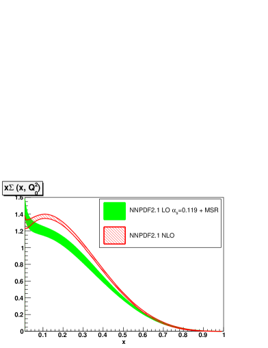
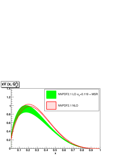
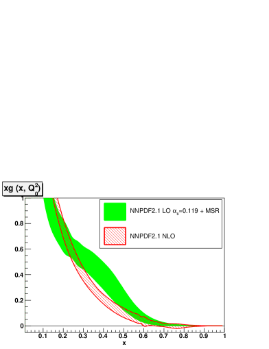
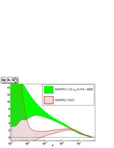
Figure 7: Comparison of the quark singlet, valence and gluon distributions for the pair of PDF fits whose distances are plotted in Fig. 6.

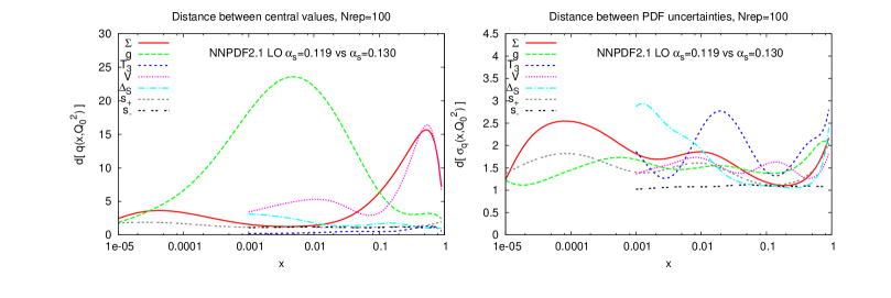
Figure 8: Distances between the NNPDF2.1 LO sets with $\alpha_{s}$=0.119 and $\alpha_{s}$=0.130.

5.3 Parton distributions

We now compare the four LO PDF sets with each other, with NLO PDFs, and with other available LO PDF sets. We will compute the distance between central values and uncertainties of the various pairs of PDFs which are being compared, defined as in Appendix A of Ref. [6]. Recall that with $N_{\rm rep}=100$ replicas a distance $d=1$ corresponds to central values which differ by ${{1}\over{\sqrt{50}}}\sigma$, with $\sigma$ the sum in quadrature of the uncertainties of the two sets. If the sets which are being compared are statistically equivalent, then all distances are of order one, while if they are statistically inequivalent but consistent at the $n$ sigma level, then distances are of order of $d\sim 7n$.

Figure 9: Comparison of the quark singlet, and gluon distributions for the pair of PDF fits whose distances are plotted in Fig. 8.

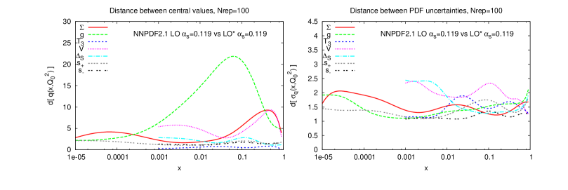
Figure 10: Distances between the NNPDF2.1 LO and LO^∗ sets with $\alpha_{s}$=0.119.

We begin by comparing the NNPDF2.1 LO set with $\alpha_{s}$=0.119, which we take as the LO reference, to the reference NNPDF2.1 NLO set. The corresponding distances are plotted in Fig. 6, while the singlet, valence and gluon PDFs are compared in Fig. 7. A full comparison of all LO, NLO and NNLO PDFs will be presented in Sect. 7.1. It is clear from Fig. 6 that LO and NLO PDF uncertainties, though clearly not statistically equivalent, are consistent at the one sigma level: this shows that these uncertainties essentially reflect the uncertainty of the underlying data, which are the same in the two PDF determinations. On the other hand, central values differ by many sigma: this means that, as already mentioned, the difference between LO and NLO PDFs is much larger than the uncertainty on either, and thus the dominant uncertainty on LO PDF is the theoretical uncertainty due to the lack of inclusion of higher order corrections.

The largest shift from LO to NLO, more than five times larger than the PDF uncertainty, is observed for the gluon at medium-small $x$ ($10^{-4}\leq x\leq 0.05$), consistent with the fact that the gluon decouples from LO observables, but also the large $x$ quark singlet and valence distributions change by more than three sigma. Generally, the LO gluon is larger than the NLO one. However, for $x\leq 10^{-4}$, where there are no data to constrain the fits, the LO and NLO gluons become consistent within the large PDF uncertainties. At larger $x$, the LO and NLO gluons are quite similar and compatible within the respective uncertainties. The LO quark is rather smaller (by more than one sigma) than the NLO one for large $x>0.1$, but it becomes compatible with it at the one sigma level for smaller $x$. Finally, the light sea and strangeness asymmetries are minimally affected and quite close at LO and NLO.

It is interesting to observe that the missing large NLO $K$-factors in Drell-Yan data should enhance the LO quark distributions in comparison to the NLO ones: the fact that they end up being instead either smaller or comparable suggests that the Drell-Yan data actually have relatively little effect on the LO fit, other than through the determination of the $\bar{u}-\bar{d}$ light flavor asymmetry. This is less sensitive to the $K$ factors (being mostly determined by a cross-section ratio), and indeed turns out to be almost the same at LO and NLO.

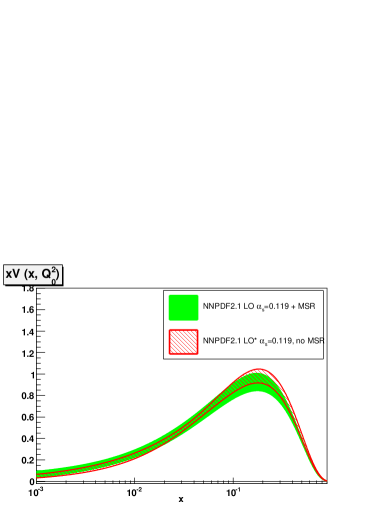
Figure 11: Comparison of the valence and gluon distributions for the pair of PDF fits whose distances are plotted in Fig. 10.

Next we compare the various LO PDF sets to each other. First we compare the two LO sets which differ in value of the strong coupling, $\alpha_{s}(M_{Z})=0.119$ vs. $\alpha_{s}(M_{Z})=0.130$. The larger value of the strong coupling, when evolved down to a scale $Q^{2}\sim 10$ GeV² using LO evolution, leads to a value of $\alpha_{s}$ close to that preferred by data in this region. Hence, the larger value leads to a better description of scaling violations at low scale, and conversely, as it is apparent from Table 4.

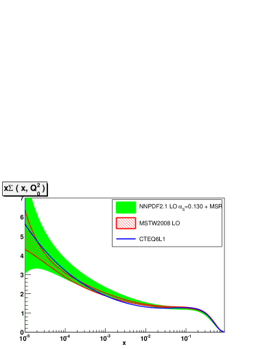
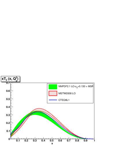
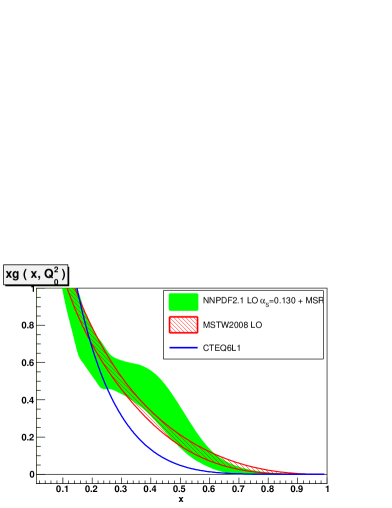
Figure 12: Comparison of LO PDFs: the quark singlet, triplet and gluon PDFs are shown for the NNPDF2.1, MSTW08 and CTEQ6L1 sets.

The distances for central values and uncertainties between the LO fits with different $\alpha_{s}$ are plotted in Fig. 8. The only PDF which is significantly affected by the value of $\alpha_{s}$ is the gluon, which, as shown in Fig. 9, becomes smaller at medium-small $x$ and thus, by the momentum sum rule, somewhat larger at large $x$ when $\alpha_{s}$ is increased. This makes the LO gluon with larger $\alpha_{s}$ closer to the NLO gluon. However, the shift as $\alpha_{s}$ is varied in this range is comparable to the PDF uncertainty. Also, the large $x$ singlet and valence quark PDFs increase somewhat when $\alpha_{s}$ is raised, especially at large $x\sim 0.3$, where a shift of about two sigma is observed.

The effect of relaxing the momentum sum rule is studied by comparing the LO and LO* sets. Those with $\alpha_{s}(M_{Z})=0.119$ are compared in Fig. 10, where the distance between them is displayed. The main difference is seen in the medium $x$ gluon, as shown in Fig. 11: the LO* gluon is rather larger than the LO one. However, the central values for all quark PDFs are very close to the standard LO ones.

In conclusion, we compare the NNPDF2.1 LO PDFs to other available LO sets. First, we compare the NNPDF2.1 LO set with $\alpha_{s}=0.130$ to MSTW08 LO [13] ($\alpha_{s}=0.139$) and CTEQ6L1 [61] ($\alpha_{s}=0.130$) in Fig. 12. Differences are especially large for the gluon distribution, both at small and large $x$, and for the isospin triplet distribution and large $x$, though differences between the NNPDF and MSTW sets are mostly compatible with the large uncertainties, while the difference between CTEQ and other sets is more difficult to quantify more precisely because CTEQ LO PDFs come without an uncertainty estimate.

Figure 13: Comparison of the NNPDF2.1 LO PDF to modified LO PDF sets: MRST2007lomod, CT09MC1, CT09MC2 and CT09MCS.

Finally we compare with the modified LO PDF sets MRST2007lomod [9], and with the dedicated Monte Carlo sets of the CTEQ/TEA collaboration [10], CT09MC1, CT09MC2 and CT09MCS. The MRST2007lomod set is obtained relaxing the momentum sum rule and using two-loop running of $\alpha_{s}$, with $\alpha_{s}(M_{z})=0.121$. The CT sets are based on an LO QCD analysis framework of data which, on top of the standard global dataset used for the NLO PDF determination, also includes a set of LHC pseudo-data generated using NLO PDFs. The normalization of the LO calculation for each pseudo-data set is allowed to float to reach the best agreement with the NLO cross-section. The CT09MCS is extracted from an analysis in which the two-loop strong coupling is used and the momentum sum rule is imposed during the fit. The CT09MC1 and CT09MC2 are fits in which the momentum sum rule is relaxed and one- and two-loop expressions for $\alpha_{s}$ are used respectively. All these sets are compared to the default NNPDF2.1 LO set in Fig. 13. Differences between these modified PDF sets are significant, and typically larger than the difference between the NNPDF2.1 LO and LO^∗ sets, consistent with the fact that they are based on different methodologies and assumptions.

6 Next-to-next-to-leading order parton distributions

Next-to-next-to-leading order PDFs are mostly of interest for their use in the computation of standard candle processes such as $W$, $Z$, top and Higgs production at hadron colliders. In this section we will discuss the statistical features of the NNLO fit, then present the NNPDF2.1 NNLO PDFs and compare them to other available NNLO sets. The implications of the NNPDF2.1 NNLO set for LHC observables are discussed in Sect. 8.

6.1 Statistical features

$\chi^{2}_{\mathrm{tot}}$	1.16
$\left\langle E\right\rangle\pm\sigma_{E}$	$2.22\pm 0.07$
$\left\langle E_{\rm tr}\right\rangle\pm\sigma_{E_{\rm tr}}$	$2.19\pm 0.09$
$\left\langle E_{\rm val}\right\rangle\pm\sigma_{E_{\rm val}}$	$2.27\pm 0.10$
$\left\langle{\rm TL}\right\rangle\pm\sigma_{\rm TL}$	$\left(17\pm 7\right)\,10^{3}$
$\left\langle\chi^{2(k)}\right\rangle\pm\sigma_{\chi^{2}}$	$1.23\pm 0.05$
$\left\langle\sigma^{(\exp)}\right\rangle_{\mathrm{dat}}$(%)	11.9
$\left\langle\sigma^{(\mathrm{net})}\right\rangle_{\mathrm{dat}}$(%)	3.2
$\left\langle\rho^{(\exp)}\right\rangle_{\mathrm{dat}}$	0.18
$\left\langle\rho^{(\mathrm{net})}\right\rangle_{\mathrm{dat}}$	0.53

Table 5: Table of statistical estimators for the NNPDF2.1 NNLO fit with $N_{\rm rep}=1000$ replicas.

Experiment	$\chi^{2}$	$\chi^{2}_{\rm nlo}$	$\left\langle E\right\rangle$	$\left\langle\sigma^{(\exp)}\right\rangle_{\mathrm{dat}}$(%)	$\left\langle\sigma^{(\mathrm{net})}\right\rangle_{\mathrm{dat}}$(%)	$\left\langle\rho^{(\exp)}\right\rangle_{\mathrm{dat}}$	$\left\langle\rho^{(\mathrm{net})}\right\rangle_{\mathrm{dat}}$
NMC-pd	0.93	0.97	1.98	1.8	0.5	0.03	0.34
NMC	1.63	1.73	2.67	5.0	1.8	0.16	0.75
SLAC	1.01	1.27	2.05	4.4	1.8	0.31	0.78
BCDMS	1.32	1.24	2.38	5.7	2.6	0.47	0.58
HERAI-AV	1.10	1.07	2.16	7.6	1.3	0.06	0.44
CHORUS	1.12	1.15	2.18	15.0	3.5	0.08	0.37
FLH108	1.26	1.37	2.25	72.1	4.8	0.65	0.68
NTVDMN	0.49	0.47	1.74	21.0	14.0	0.04	0.64
ZEUS-H2	1.31	1.29	2.33	14.0	1.3	0.28	0.55
ZEUSF2C	0.88	0.78	1.89	23.0	3.7	0.07	0.40
H1F2C	1.46	1.50	2.48	18.0	3.5	0.27	0.36
DYE605	0.81	0.84	1.88	25.0	7.2	0.55	0.76
DYE866	1.32	1.27	2.40	21.0	8.7	0.23	0.48
CDFWASY	1.65	1.86	2.80	6.0	4.3	0.52	0.61
CDFZRAP	2.12	1.65	3.21	12.0	3.6	0.82	0.67
D0ZRAP	0.67	0.60	1.69	10.0	3.0	0.54	0.70
CDFR2KT	0.74	0.97	1.84	23.0	4.8	0.77	0.61
D0R2CON	0.82	0.84	1.89	17.0	5.5	0.78	0.62

Table 6: Same as Table 5 for individual experiments. All estimators have been obtained with $N_{\rm rep}=1000$ replicas. Note that experimental uncertainties are always given in percentage. For reference we also provide the NNPDF2.1 NLO $\chi^{2}$ for the various experiments.

Statistical estimators for the NNPDF2.1 NNLO fit are shown in Table 5 for the global fit and in Table 6 for individual experiments, with, in the latter case, the NLO $\chi^{2}$ values also shown for comparison. While referring to Refs. [6, 8, 62, 60] for a detailed discussion of statistical indicators and their meaning, we recall that $\chi^{2}_{\mathrm{tot}}$ is computed comparing the central (average) NNPDF2.1 fit to the original experimental data, $\left\langle\chi^{2(k)}\right\rangle$ is computed comparing to the data each NNPDF2.1 replica and averaging over replicas, while $\left\langle E\right\rangle$ is the quantity which is minimized, i.e. it coincides with the $\chi^{2}$ computed comparing each NNPDF2.1 replica to the data replica it is fitted to, with the three values given corresponding to the total, training, and validation datasets.

Figure 14: Distribution of $\chi^{2(k)}$ (left) and $E^{(k)}_{\rm tr}$ (right), over the sample of $N_{\mathrm{r}ep}=1000$ replicas.

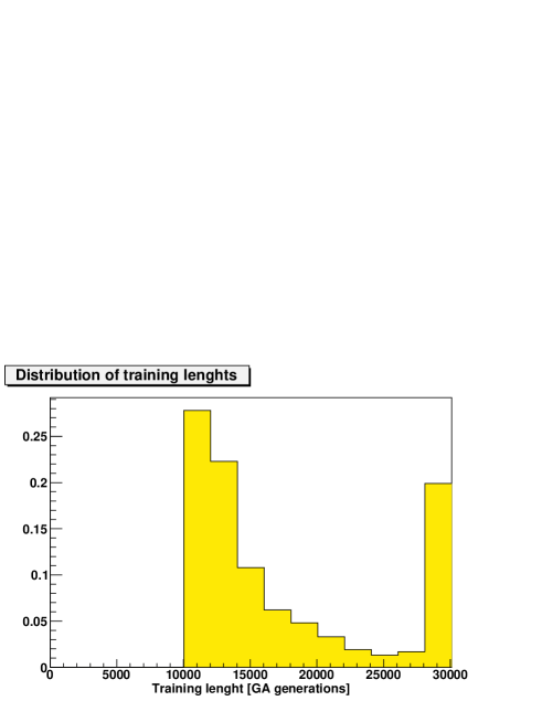
Figure 15: Distribution of training lengths over the sample of $N_{\mathrm{r}ep}=1000$ replicas.

All statistical indicators (including the training length), and in particular the quality of the global fit as measured by the value $\chi^{2}_{\mathrm{tot}}=1.16$ are quite similar to those of the NLO fit. Specifically, the NLO and NNLO $\chi^{2}$ differ by less than 10% for all experiments, except SLAC, the $W$ asymmetry and CDF jet data (for which NNLO is better) and the $Z$ rapidity distribution (for which it is worse). It is interesting to observe that an excellent description of the HERA $F_{2}^{c}$ data is obtained without the need of any ad hoc cut or tuning of the treatment of heavy quarks (the NNLO $\chi^{2}$ is somewhat worse than the NLO one, but at NNLO the dataset is considerably wider, as discussed in Sect. 2.2).

The distribution of $\chi^{2(k)}$, $E^{(k)}_{\rm tr}$, and training lengths among the $N_{\rm rep}=1000$ NNPDF2.1 NNLO replicas are shown in Fig. 14 and Fig. 15 respectively. While most of the replicas fulfill the stopping criterion, a fraction ($\sim 20\%$) of them stops at the maximum training length $N_{\rm gen}^{\rm max}$ which has been introduced in order to avoid unacceptably long fits. This fraction is comparable but somewhat larger than the corresponding NLO one. In order to check that this causes no significant loss of accuracy, we have verified that if all replicas that do not stop dynamically are discarded, the PDF change by an amount which is smaller than a statistical fluctuation. We have also verified that this fraction is reduced if the maximum training length is raised, thereby showing that the issue is merely one of computational efficiency, rather than principle.

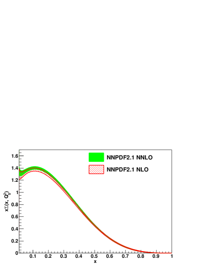
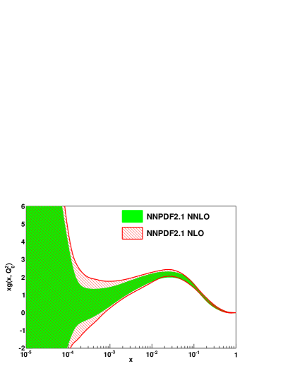
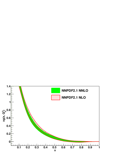
Figure 16: Comparison of NNPDF2.1 NLO and NNLO singlet sector PDFs, computed using $N_{\rm rep}=1000$ replicas from both sets. All error bands shown correspond to one sigma.

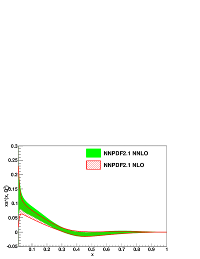
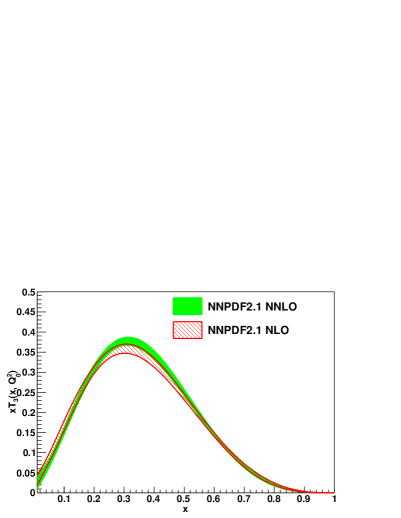
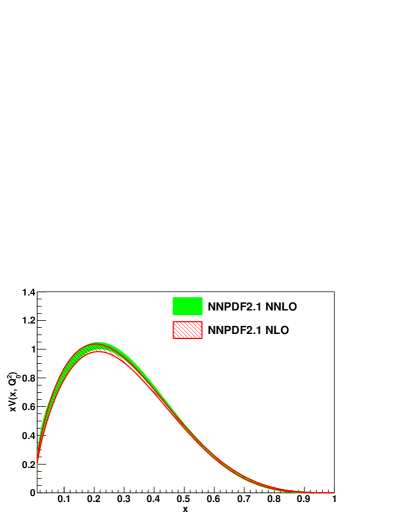
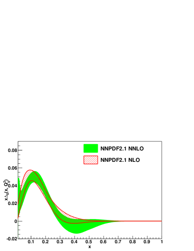
Figure 17: Same as Fig. 16 for the non–singlet sector PDFs.

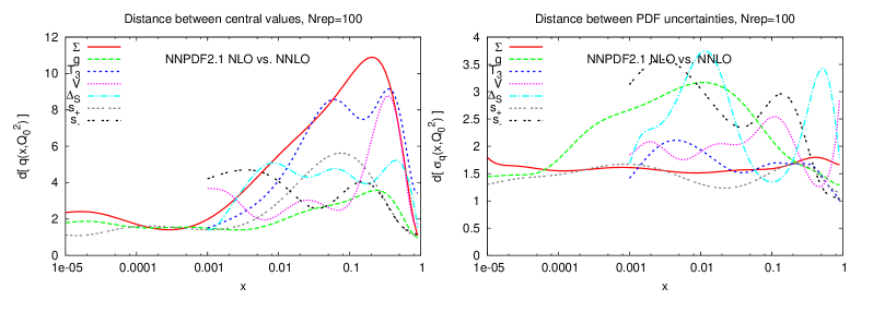
Figure 18: Distances between the NNPDF2.1 NLO and NNLO parton sets shown in Figs. 16 and 17. All distances are computed from sets of $N_{\rm rep}=100$ replicas.

6.2 Parton distributions

The NNPDF2.1 NNLO parton distributions are shown along with their NLO counterparts in Figs. 16 and 17 at the input scale $Q_{0}^{2}=2$ GeV², in the basis in which they are parametrized. The distances (defined as in Appendix A of Ref. [6]) between the NLO and NNLO sets are shown in Fig. 18.

Recalling that a distance $d\sim 1$ corresponds to statistical equivalence, while (with 100 replicas) $d\sim 7$ is a one sigma shift, it is apparent that the NLO and NNLO sets are statistically inequivalent, but differ by typically less than one sigma. This in particular means that PDFs in the NNPDF2.1 set are quite stable when going from NLO to NNLO. The largest variations are observed for quarks at $x\sim 0.1$, while the small $x$ PDFs (gluon and light quark sea) are very similar to their NLO counterparts. It is worth noting that the distances for the PDF uncertainties in Fig. 18 are particularly small. This is as it should be, consistently with the fact that the quality of the NLO and NNLO fits are similar, given that theory uncertainties are not included in PDF uncertainties.

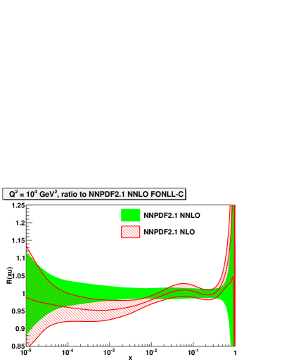
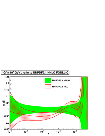
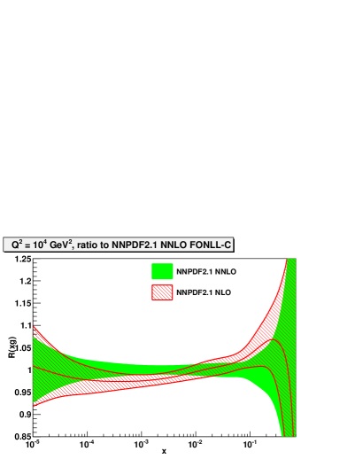
Figure 19: Comparison between NNPDF2.1 NLO and NNLO light quark and gluon PDFs at $Q^{2}=10^{4}$ GeV². The results have been obtained with $N_{\rm rep}=1000$ replicas. All curves are shown as ratios to the central NNPDF2.1 NNLO result.

In order to assess the impact of NNLO corrections on physical observables it is useful to compare NNLO and NLO PDFs for individual flavours at a typical hard scale. This is done in Fig. 19, where the NNLO/NLO ratio is shown as a function of $x$ at $Q^{2}=10^{4}$ GeV². The most noticeable changes are larger small $x$ quarks (and correspondingly, due to evolution, larger small $x$ gluons) and smaller large $x$ quarks. The biggest differences are observed for the light quark sea at $x\sim 10^{-3}$, where the NNLO and NLO bands just about miss each other.

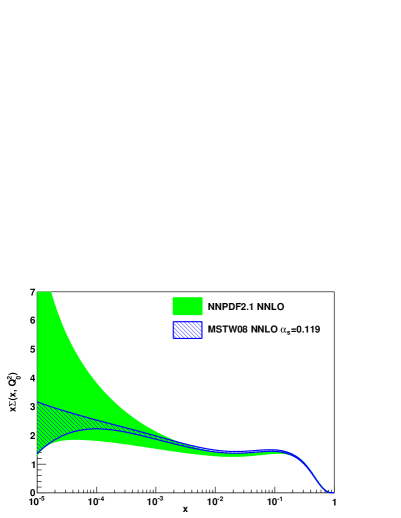
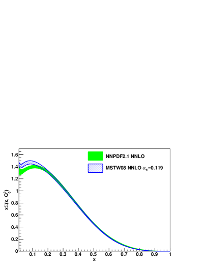
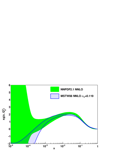
Figure 20: The NNPDF2.1 NNLO singlet sector PDFs, compared to MSTW08 PDFs. The results for NNPDF2.1 NNLO have been obtained with $N_{\rm rep}=1000$ replicas. All PDF errors are given as one sigma uncertainties. In the comparison a common value of $\alpha_{s}\left(M_{Z}\right)$=0.119 has been used.

Next, in Figs. 20 and 21 we compare the NNPDF2.1 NNLO PDFs to those from the MSTW08 NNLO set. For consistency we use in the comparison a common value of $\alpha_{s}\left(M_{Z}\right)$=0.119. The MSTW08 NNLO gluon, unlike its NNPDF2.1 counterpart, is unstable at small $x$, where it becomes very negative. For other PDFs there is reasonable agreement for central values, although the uncertainty bands from MSTW often seem unusually small. Sizable differences are observed in the strange distribution, but it should be recalled that in MSTW08 the parametrization of the $s+\bar{s}$ and especially $s-\bar{s}$ PDF is extremely restrictive, while in NNPDF2.1 they are treated on the same footing as the other PDFs.

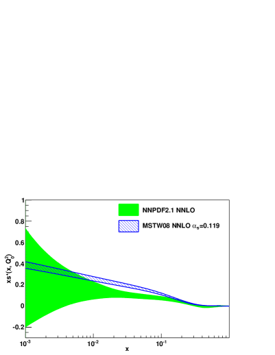
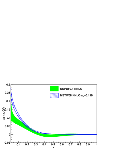
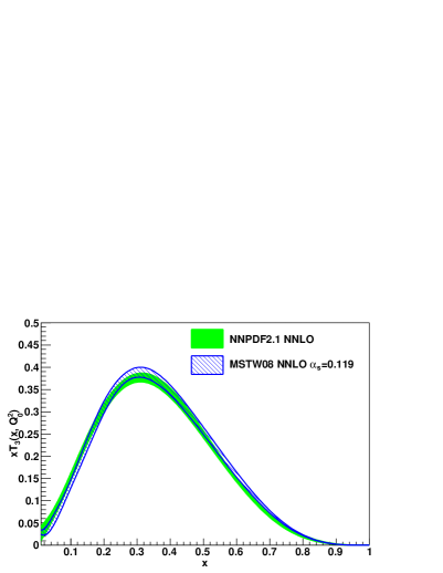
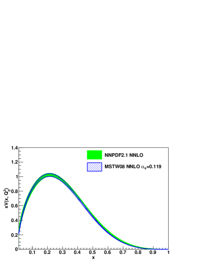
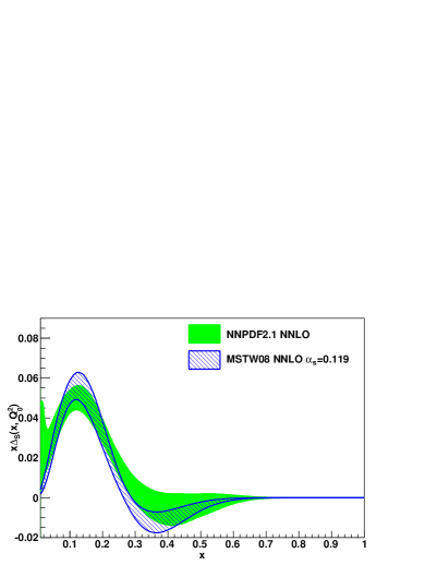
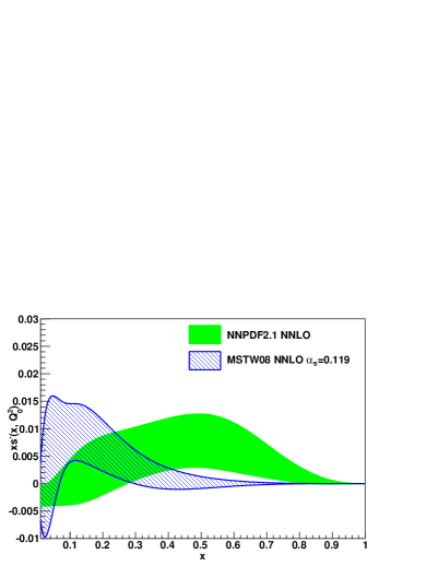
Figure 21: Same as Fig. 20 for the non–singlet sector PDFs.

At present, MSTW08 is the only NNLO PDF set which is publicly available through the LHAPDF [63, 64] interface for a variety of values of $\alpha_{s}$. However, it may also be interesting to compare the NNPDF2.1 NNLO PDFs to the ABKM09 NNLO set (with fixed flavour number $n_{f}=3$) [65]. This set is only provided for $\alpha_{s}\left(M_{Z}\right)=0.1135\pm 0.0014$, furthermore for this set (and its NLO counterpart) only combined PDF+$\alpha_{s}$ uncertainties can be determined, unlike other sets for which PDF uncertainties with fixed $\alpha_{s}$ may also be computed. The comparison is shown in Figs. 22 and  23 at $Q_{0}^{2}=$ 2 GeV², where we have chosen the NNPDF2.1 set with $\alpha_{s}=0.114$ in order to make the comparison more significant. Even so, the agreement is generally not very good.

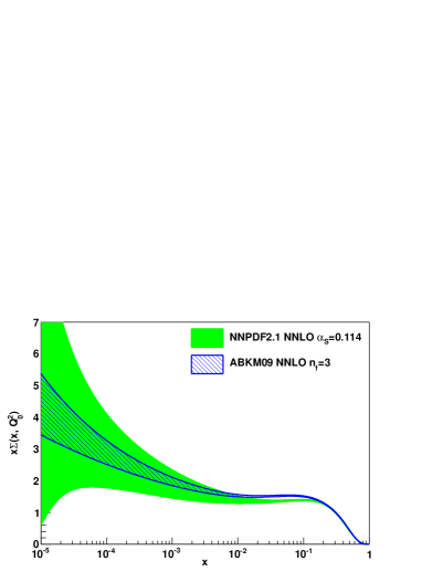
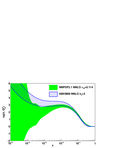
Figure 22: The NNPDF2.1 NNLO singlet sector PDFs, compared to the ABKM09 three-flavor set. The results for NNPDF2.1 NNLO have been obtained with $N_{\rm rep}=100$ replicas. The NNPDF2.1 set with $\alpha_{s}=0.114$ is shown because ABKM PDFs are only available for this value of $\alpha_{s}$. Note that for ABKM uncertainties also include the uncertainty on $\alpha_{s}$ while for NNPDF they are pure PDF uncertainties.

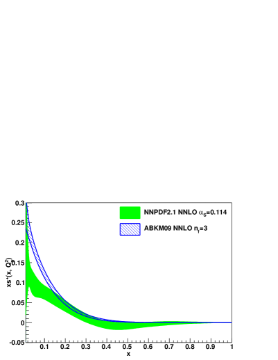
Figure 23: Same as Fig. 22 for the non–singlet sector PDFs.

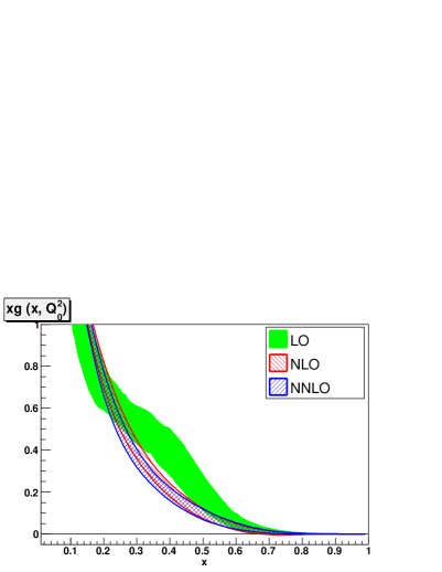
Figure 24: Comparison of NNPDF2.1 LO, NLO and NNLO singlet sector PDFs at $Q_{0}^{2}$=2 GeV². All uncertainty bands are defined as 68% confidence levels.

7 Perturbative stability

With PDF sets at LO, NLO and NNLO determined from the same data and using a uniform methodology we can address issues of perturbative stability. We will do this first by comparing individual PDFs, and then by looking at the behaviour of the total momentum fraction carried by partons.

7.1 Parton distributions

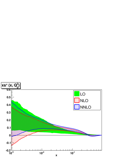
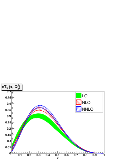
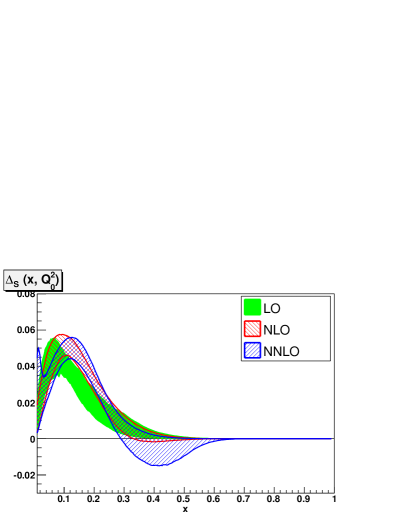
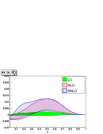
Figure 25: Same as Fig. 24 for the non-singlet sector PDFs.

We assess the perturbative stability of the PDF determination by comparing the NNPDF2.1 PDFs as they go from LO to NNLO accuracy in perturbative QCD. The LO, NLO and NNLO NNPDF2.1 PDFs are compared in Figs. 24 and 25 at the starting scale $Q_{0}^{2}$=2 GeV² in the basis in which they are independently parametrized by neural networks. All error bands shown are defined as 68% confidence levels, rather than as standard deviations, so that possible deviations from gaussian behaviour are accounted for. In Figs. 26 and 27 we provide a similar comparison but this time at the scale $Q^{2}$= (100 GeV)² in the basis of individual flavours.

The excellent convergence of the perturbative expansion within the kinematic region covered by the experimental data is clear from these plots. In particular, even in the small $x$ and large $x$ region, where we expect perturbation theory to become unstable and resummation to be necessary [66, 67], no evidence of instability is seen in the PDFs, thus suggesting that resummation corrections are smaller than current PDF uncertainties (at small $x$, this is borne out by the dedicated study of Refs. [68, 69]).

It is also clear that the NNLO and NLO results for all PDFs almost always agree within uncertainties. In particular, with one single exception, at the starting scale (Figs. 24-25) the NNLO central value is within (or just outside) the NLO uncertainty band, and in fact it differs from the NLO central value by an amount which is usually much smaller than the NLO uncertainty. The exception is the isospin triplet distribution around the valence peak $x\sim 0.3$, where the NLO and NNLO bands overlap, but the NNLO central value is clearly outside the NLO band. At a higher scale (Figs. 26-27) the situation further improves, and the NLO and NNLO results become almost indistinguishable, and only the small discrepancy in light quark distributions for $x\mathrel{\hbox to0.0pt{\lower 4.0pt\hbox{\hskip 1.0pt$\sim$}\hss}\raise 1.0pt\hbox{$>$}}10^{-3}$ already observed in Fig. 19 remains.

This leads to an important conclusion. At present, the PDF uncertainties provided by NNPDF, and indeed all other PDF groups, only reflect the data uncertainties: in particular they do not include the theoretical uncertainty due to higher perturbative orders, which could be estimated by varying the renormalization and factorization scale during the PDF fit. At NLO we can estimate the theoretical uncertainty by a direct comparison with the NNLO results. This comparison shows that at NLO (and beyond) it is at present generally a reasonable approximation to neglect the theoretical uncertainty, since it is usually smaller than the PDF uncertainty coming from uncertainties in the data.

On the other hand, at the starting scale the LO PDFs differ by many standard deviations from NLO PDFs. One must conclude that at LO the PDF uncertainty provided with NNPDF PDFs (as well as with any other available LO set) is only a fraction of the total uncertainty, the theoretical component here being the dominant one. The situation improves somewhat at high scale (Figs. 26-27), but the difference between LO and NLO remains large for the gluon.

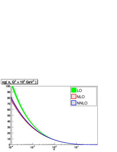
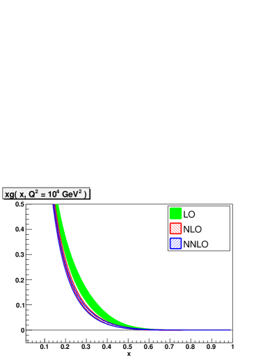
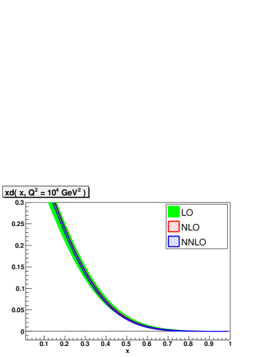
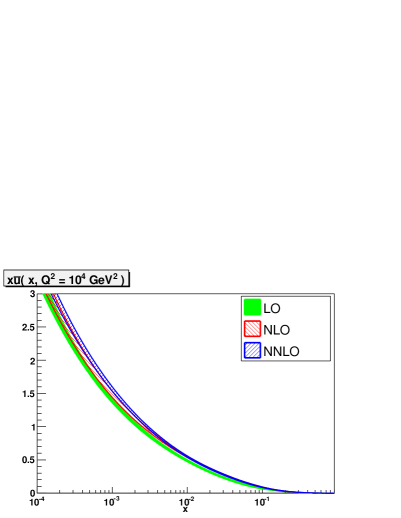
Figure 26: Comparison of NNPDF2.1 LO, NLO and NNLO PDFs in the flavour basis at $Q^{2}=10^{4}$ GeV²: light quarks and gluon.

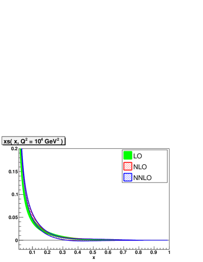
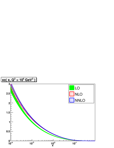
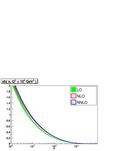
Figure 27: Comparison of NNPDF2.1 LO, NLO and NNLO PDFs in the flavour basis at $Q^{2}=10^{4}$ GeV²: strange and heavy quarks.

Finally, all seven independently parametrized LO, NLO and NNLO PDFs are collected in a single plot in Fig. 28 at a low scale $Q^{2}$=2 GeV² and in Fig. 29 at higher scale $Q^{2}=10^{4}$ GeV². These plots illustrate the relative size of individual PDFs. Note that at high scale the plot has a log scale on the vertical axis because due to perturbative evolution the different PDFs can differ by several orders of magnitude.

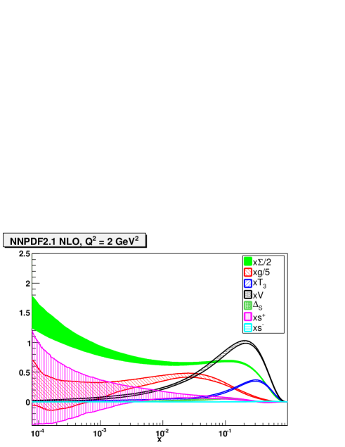
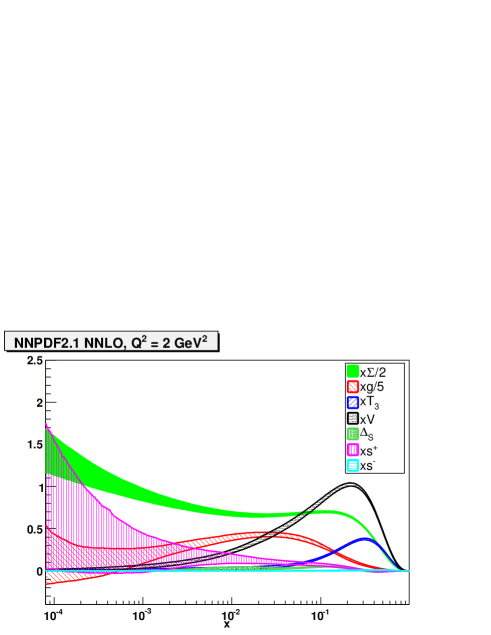
Figure 28: Summary of the NNPDF2.1 LO (top), NLO (center) and NNLO (bottom) PDF sets at $Q^{2}$=2 GeV². All uncertainty bands are defined as 68% confidence levels.

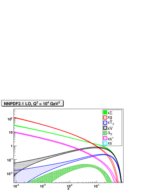
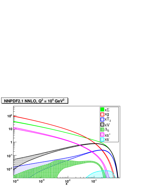
Figure 29: Same as Fig.28 at $Q^{2}=10^{4}$ GeV². Note the logarithmic scale on the $y$ axis.

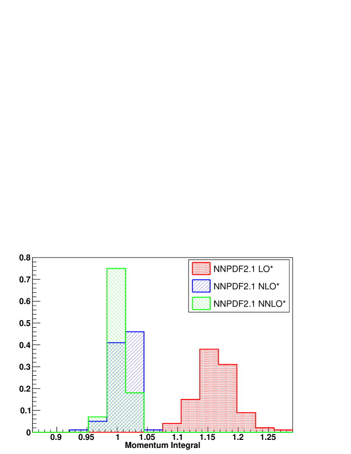
Figure 30: Distribution of total momentum integrals for the $N_{\rm rep}=100$ replicas in the NNPDF2.1 LO*, NLO* and NNLO* PDF sets; $\alpha_{s}(M_{z})=$0.119 in all cases.

7.2 The momentum of quarks and gluons in the nucleon

The value of the total momentum carried by quarks and gluons and its dependence on the perturbative order provide a strong consistency check of the perturbative QCD framework. With the aim of testing this, we have performed NLO and NNLO PDF determinations in which the momentum sum rule is relaxed, denoted as NLO* and NNLO*, which supplement the LO* fit of Sect. 5. We take $\alpha_{s}(M_{Z})=$0.119 at all perturbative orders. In all cases, we find that the fit quality is not changed in a significant way when relaxing the momentum sum rule.

The momentum fraction carried by a parton distribution is

$$\left[q\right]\left(Q^{2}\right)\equiv\int_{0}^{1}dx\,xq\left(x,Q^{2}\right)\ .$$ (4)

Using the LO*, NLO* and NNLO* PDF sets, we find that the total momentum $\left[M\right]=\left[\Sigma\right]+\left[g\right]$ carried by partons is

$$\left[M\right]_{\rm LO}=1.161\pm 0.032\,,$$

$$\left[M\right]_{\rm NLO}=1.011\pm 0.018\,,$$ (5)

$$\left[M\right]_{\rm NNLO}=1.002\pm 0.014\,.$$

where the uncertainty is only from PDFs (and thus does not include any theoretical uncertainty). The distributions of total momentum integrals over the 100 replicas for the NNPDF2.1 LO*, NLO* and NNLO* sets is shown in Fig. 30: they appear to be Gaussian to a good approximation.

Estimating the theoretical uncertainty as the difference between results at two subsequent perturbative orders, we see that at LO the theoretical uncertainty is dominant, as we already concluded from the PDF plots Figs. 24-25 in Sect. 7. The deviation of the LO momentum integral from the QCD prediction is mostly driven by the gluon, which turns out to be larger in the LO* set than in the default LO set with momentum sum rule imposed. On the other hand already at NLO the theoretical uncertainty is half of the PDF uncertainty, $\Delta^{\rm th}\left[M\right]_{\rm NLO}=0.01$, and thus at NNLO the theoretical uncertainty is likely to be negligible.

PDF combination	LO*	NLO*	NNLO*
$\left[\Sigma+g\right]$	$1.161\pm 0.032$	$1.011\pm 0.018$	$1.002\pm 0.014$
$Q^{2}_{0}=2$ GeV2
$\left[\Sigma\right](Q_{0}^{2})$	$0.550\pm 0.025$	$0.591\pm 0.010$	$0.602\pm 0.010$
$\left[g\right](Q^{2}_{0})$	$0.612\pm 0.028$	$0.421\pm 0.021$	$0.400\pm 0.018$
$\left[\left(u+\bar{u}\right)\right](Q^{2}_{0})$	$0.346\pm 0.015$	$0.371\pm 0.005$	$0.376\pm 0.005$
$\left[\left(d+\bar{d}\right)\right](Q^{2}_{0})$	$0.192\pm 0.011$	$0.206\pm 0.005$	$0.209\pm 0.003$
$\left[\left(s+\bar{s}\right)\right](Q^{2}_{0})$	$0.012\pm 0.004$	$0.014\pm 0.006$	$0.017\pm 0.006$
$Q^{2}=10^{4}$ GeV2
$\left[\Sigma\right](Q^{2})$	$0.546\pm 0.017$	$0.528\pm 0.009$	$0.527\pm 0.005$
$\left[g\right](Q^{2})$	$0.615\pm 0.020$	$0.486\pm 0.018$	$0.475\pm 0.011$
$\left[\left(u+\bar{u}\right)\right](Q^{2})$	$0.264\pm 0.009$	$0.256\pm 0.003$	$0.255\pm 0.002$
$\left[\left(d+\bar{d}\right)\right](Q^{2})$	$0.165\pm 0.007$	$0.160\pm 0.002$	$0.159\pm 0.001$
$\left[\left(s+\bar{s}\right)\right](Q^{2})$	$0.048\pm 0.003$	$0.047\pm 0.004$	$0.048\pm 0.004$
$\left[\left(c+\bar{c}\right)\right](Q^{2})$	$0.041\pm 0.002$	$0.039\pm 0.002$	$0.039\pm 0.001$
$\left[\left(b+\bar{b}\right)\right](Q^{2})$	$0.027\pm 0.001$	$0.025\pm 0.001$	$0.025\pm 0.001$

Table 7: Momentum fractions of various PDF combinations at low scale $Q_{0}^{2}=2$ GeV² and high scale $Q^{2}=10^{4}$ GeV² when the momentum sum rule is not imposed (LO*, NLO* and NNLO* PDF sets). All results are obtained with $N_{\rm rep}=100$ replicas.

PDF combination	LO	NLO	NNLO
$\left[\Sigma+g\right]$	$1$	$1$	$1$
$Q^{2}_{0}=2$ GeV2
$\left[\Sigma\right](Q_{0}^{2})$	$0.521\pm 0.023$	$0.590\pm 0.009$	$0.609\pm 0.013$
$\left[g\right](Q^{2}_{0})$	$0.479\pm 0.022$	$0.411\pm 0.009$	$0.391\pm 0.012$
$\left[\left(u+\bar{u}\right)\right](Q^{2}_{0})$	$0.328\pm 0.012$	$0.371\pm 0.005$	$0.381\pm 0.007$
$\left[\left(d+\bar{d}\right)\right](Q^{2}_{0})$	$0.181\pm 0.010$	$0.206\pm 0.004$	$0.211\pm 0.005$
$\left[\left(s+\bar{s}\right)\right](Q^{2}_{0})$	$0.012\pm 0.005$	$0.013\pm 0.006$	$0.017\pm 0.005$
$Q^{2}=10^{4}$ GeV2
$\left[\Sigma\right](Q^{2})$	$0.492\pm 0.010$	$0.523\pm 0.003$	$0.529\pm 0.004$
$\left[g\right](Q^{2})$	$0.509\pm 0.010$	$0.477\pm 0.003$	$0.471\pm 0.005$
$\left[\left(u+\bar{u}\right)\right](Q^{2})$	$0.245\pm 0.007$	$0.255\pm 0.003$	$0.257\pm 0.004$
$\left[\left(d+\bar{d}\right)\right](Q^{2})$	$0.150\pm 0.006$	$0.159\pm 0.002$	$0.159\pm 0.002$
$\left[\left(s+\bar{s}\right)\right](Q^{2})$	$0.041\pm 0.003$	$0.046\pm 0.003$	$0.048\pm 0.002$
$\left[\left(c+\bar{c}\right)\right](Q^{2})$	$0.033\pm 0.001$	$0.0383\pm 0.0004$	$0.0393\pm 0.0006$
$\left[\left(b+\bar{b}\right)\right](Q^{2})$	$0.021\pm 0.001$	$0.0245\pm 0.0002$	$0.0249\pm 0.0003$

Table 8: Same as Table 7, but when the momentum sum rule is imposed (LO, NLO and NNLO PDF sets).

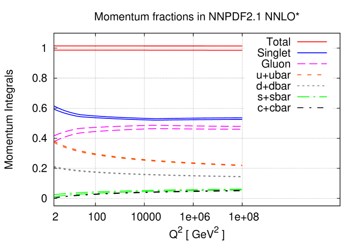
Figure 31: Momentum fractions carried by various combinations of quark and gluon distributions as a function of the scale $Q^{2}$ at NNLO, when the momentum sum rule is (top) or is not (bottom) imposed.

It is also interesting to determine the momentum fraction carried by individual PDFs. These are tabulated in Tables 7-8 at a low scale $Q^{2}_{0}=2$ GeV² and at a high scale $Q^{2}=10^{4}$ GeV², both before (Table 7, * PDF sets) and after (Table 8, standard PDF sets) imposing the momentum sum rule. They are also plotted as a function of scale in Fig. 31. We show the momentum fractions of the light quarks, the gluon, and the total quark singlet combination.

The asymptotic values of the momentum carried by the total quark and gluon distributions are predicted in perturbative QCD to be

$$\lim_{Q^{2}\to\infty}[\Sigma](Q^{2})={{3n_{f}}\over{16+3n_{f}}}\approx 0.5294; \lim_{Q^{2}\to\infty}[g](Q^{2})={{16}\over{16+3n_{f}}}\approx 0.4706$$ (6)

(see e.g. Ref. [70]). The results of Tables 7-8 are in impressive agreement with the QCD prediction Eq. (6). When the momentum sum rule is imposed (Table 8) the accuracy of the determination of each momentum component improves, and the agreement with the QCD prediction Eq. (6) improves accordingly. In Fig. 32 we compare for the NNPDF2.1 NNLO and NNLO* fits the gluon and singlet momentum fraction and their ratio with the corresponding asymptotic values predicted by pQCD. This confirms the excellent agreement, both with and without the momentum sum rule imposed.

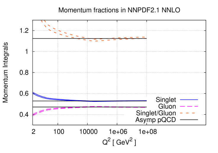
Figure 32: Momentum fractions carried by quarks and gluons, and their ratio, as a function of the scale $Q^{2}$ at NNLO, when the momentum sum rule is (top) or is not (bottom) imposed, compared to the asymptotic pQCD predictions, Eq. (6).

It is interesting to observe that even though the limits Eq. (6) hold at any perturbative order, because of asymptotic freedom, the results of Tables 7-8 agree better with the limits as the perturbative order increases. This is due to the fact that the uncertainties given in the tables do not include the theoretical uncertainty, which decreases as the perturbative order increase. Indeed, comparison of central values of the various momentum fractions at subsequent perturbative orders shows that at NLO this uncertainty is small, but not entirely negligible, as already concluded in Sect. 7.1, while at NNLO it is likely much less than the PDF uncertainties.

8 Phenomenological implications

We will now present the parton luminosities determined from NNPDF2.1 NNLO PDFs, and use them to compute several LHC standard cross-sections. As we shall see, the first LHC data already have discriminating power between existing PDF sets. They are thus likely to lead to a substantial improvement in PDF accuracy in the near future.

8.1 Parton luminosities

At a hadron collider, all factorized observables depend on parton distributions through a parton luminosity, which, following Ref. [59], we define as

$$\Phi_{ij}\left(M_{X}^{2}\right)={{1}\over{s}}\int_{\tau}^{1}{{dx_{1}}\over{x_{1}}}f_{i}\left(x_{1},M_{X}^{2}\right)f_{j}\left(\tau/x_{1},M_{X}^{2}\right)\ ,$$ (7)

where $f_{i}(x,M^{2})$ is a PDF and $\tau\equiv M_{X}^{2}/s$. Therefore, a good deal of information on the dependence of hadron-level cross-sections on PDFs can be gathered by simply looking at the luminosities which correspond to individual parton subprocesses. We consider in particular the gluon-gluon luminosity, the total quark-gluon and quark-antiquark luminosities defined as

$$\Phi_{qg}\equiv\sum_{i=1}^{n_{f}}\Phi_{q_{i}g};\quad\Phi_{q\bar{q}}\equiv\sum_{i=1}^{n_{f}}\Phi_{q_{i}\bar{q}_{i}},$$ (8)

and the charm and beauty quark-antiquark luminosities.

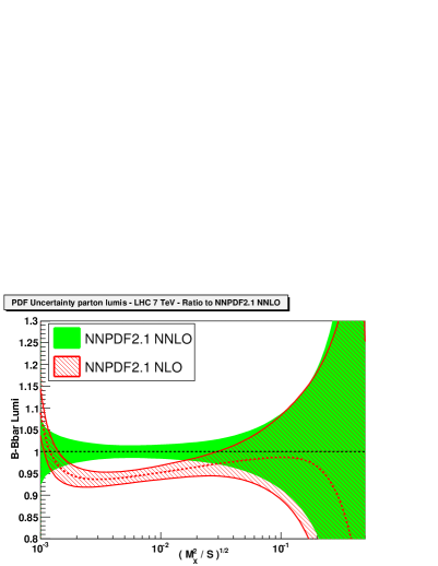
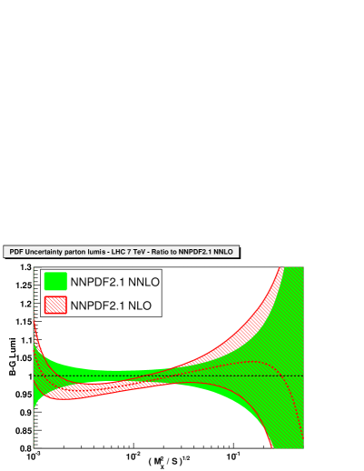
Figure 33: Comparison of the parton luminosities Eqs. (7-8) for LHC at 7 TeV, computed using the NNPDF2.1 NLO and NNLO PDFs, using $N_{\rm rep}=100$ replicas from both sets. From left to right we show $\Phi_{gg}$, $\Phi_{qg}$, (top) $\Phi_{q\bar{q}}$, $\Phi_{c\bar{c}}$, (middle) $\Phi_{b\bar{b}}$, $\Phi_{bg}$ (bottom). All luminosities are plotted as ratios to the NNPDF2.1 NNLO central value. All uncertainties shown are one sigma.

The luminosities computed from the NLO and NNLO NNPDF2.1 PDF sets are compared in Fig. 33, all normalized to the NNPDF2.1 NNLO central value. The compatibility, and thus the perturbative stability, is good for of all luminosities, as expected from the PDF comparison of Figs. 16-18. In particular, the gluon-gluon luminosity, which is relevant for Higgs production at the LHC, is quite stable in the region which corresponds to standard Higgs production, though for larger invariant masses the NNLO luminosity becomes smaller. Non-negligible differences are seen for the quark-antiquark luminosity, which is significantly larger at NNLO in the region relevant for $W$ and $Z$ production, as a consequence of the discrepancy in light quark distributions already noted in Fig. 19, which gets squared at the level of luminosities. Similar but somewhat smaller differences are seen in the quark-gluon channel. The heavy quark PDFs follow the behaviour of the gluon, from which they are generated dynamically via perturbative evolution. Note that the masses of the heavy quarks $m_{c}$ and $m_{b}$ are the same in the NLO and NNLO analyses.

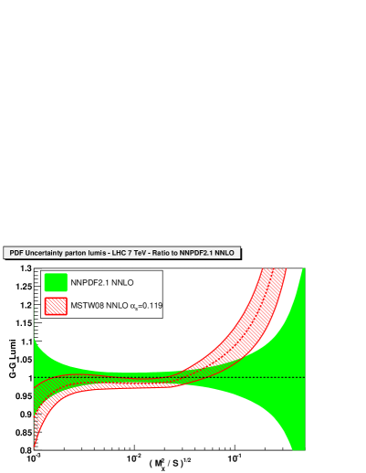
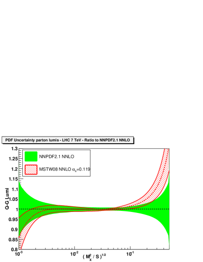
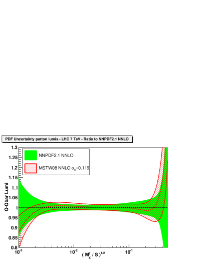
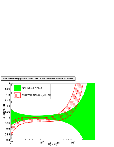
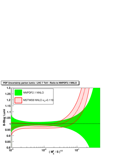
Figure 34: Same as Fig. 33, but for NNPDF2.1 NNLO and MSTW2008 NNLO PDFs. For both sets PDFs corresponding to the same value $\alpha_{s}=0.119$ have been used for consistency.

In Fig. 34 the NNPDF2.1 NNLO luminosities are compared to MSTW08 NNLO (at a common value of $\alpha_{s}=0.119$), all plotted as ratios to the NNPDF2.1 NNLO central value. The agreement is generally quite good in the region of $M_{X}^{2}/s$ which corresponds to typical electroweak final state masses $M_{X}$ at the LHC, but it deteriorates for very low and especially very high $M_{X}$. This is mostly a consequence of the strikingly different behaviour of the singlet and especially the gluon distribution at small $x$ seen in Fig. 20, related to the unstable behaviour of the MSTW08 NNLO gluon.

8.2 Predictions for LHC observables

NNLO computations are at the current frontier of perturbative QCD, and are thus available for only a small number of processes. We will now present NNLO results for the total cross-section for Higgs and weak vector boson production. We will consider also the approximate NNLO computation of the $t\bar{t}$ production cross-section.

When comparing predictions for physical observables with the aim of understanding their dependence on PDFs and their associated uncertainty it is important not to mix the uncertainties due to PDFs with uncertainties due to the choice of external parameters [71]. In particular, collider observables have a nontrivial dependence on the value of the strong coupling, both through the hard matrix elements and due to the correlation of PDFs with the value of $\alpha_{s}$ [72, 73, 74], which is particularly significant for the gluon distribution. As a consequence, as already discussed in Sect. 6, the only NNLO PDF set with which a detailed quantitative comparison is currently possible is MSTW08. For the sake of illustration, however, we will also present comparisons with the ABKM09 NNLO set, even though it should be kept in mind that these PDFs are provided for $\alpha_{s}(M_{Z})=0.1135\pm 0.0014$, and their uncertainties always include also the uncertainty due to the variation of $\alpha_{s}$ in this range.

Figure 35: The total cross-section for Higgs boson production via gluon fusion at NNLO as a function of $m_{H}$. Results are shown for NNPDF2.1 with $\alpha_{s}(M_{Z})=0.119$ and $\alpha_{s}(M_{Z})=0.117$, MSTW08 with $\alpha_{s}(M_{Z})=0.1171$, and ABKM09 with $\alpha_{s}(M_{Z})=0.1135\pm 0.0014$, all displayed as ratios to the central NNPDF2.1 curve. The NNPDF result is obtained using $N_{\rm rep}=100$ replicas. All uncertainties shown are one sigma; for NNPDF and MSTW they are pure PDF uncertainties, while for ABKM they also include the $\alpha_{S}$ uncertainty corresponding to their given range.

We consider first the total inclusive cross-section for Higgs production from gluon-gluon fusion, whose dependence on PDFs has attracted considerable attention recently, in view of claims in the literature (see Ref. [75] and references therein) that the recommended [76] determination of PDF uncertainties through the so-called PDF4LHC prescription [77] might be substantially underestimated (see Refs. [45] and especially Ref. [49] for a thorough discussion of this issue). We have computed the NNLO Higgs production cross-section in the gluon fusion channel using the code of Refs. [78, 79]. Results are shown in Fig. 35 as a function of the Higgs mass $m_{H}$, determined using the NNLO NNPDF2.1, MSTW08 and ABKM09 PDF sets. The predictions for each group are shown at the respective default value of $\alpha_{s}$, namely $\alpha_{s}(M_{Z})=0.119$ for NNPDF, $\alpha_{s}(M_{Z})=0.1171$ for MSTW08 and $\alpha_{s}(M_{Z})=0.1135\pm 0.0014$ for ABKM09; for NNPDF the prediction for $\alpha_{s}(M_{Z})=0.117$ is also shown in order to allow for a direct comparison with MSTW08 (NNPDF2.1 NNLO predictions for more values of $\alpha_{s}$ are shown and discussed in Fig. 39 of Sect. 9.1 below). All uncertainties shown are one sigma PDF uncertainties only (but in the case of ABKM, as mentioned, they include also the uncertainty on $\alpha_{s}$). The NNPDF and MSTW results are in excellent agreement, provided the same value of $\alpha_{s}$ is used. On the other hand, the ABKM result disagrees by many standard deviations: even though a sizable fraction of this disagreement is due to the different value of $\alpha_{s}$, it would persist even when the same value of $\alpha_{s}$ is adopted (see Fig. 39 below).

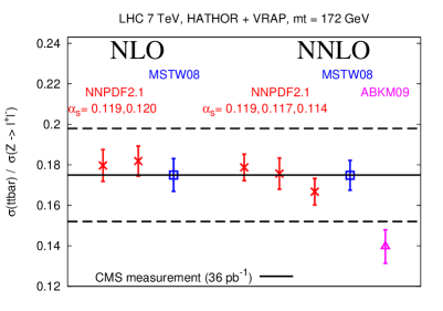
Figure 36: The total cross-section for $t\bar{t}$ production at the LHC 7 TeV computed using HATHOR (left) and its ratio to the total $Z$ production cross-section computed using VRAP (right). Results are shown for NNPDF2.1 with $\alpha_{s}(M_{Z})=0.119$ (NLO and NNLO), $\alpha_{s}(M_{Z})=0.120$ (NLO) and $\alpha_{s}(M_{Z})=0.114,0.117$ (NNLO), MSTW08 with $\alpha_{s}(M_{Z})=0.1202$ (NLO) and $\alpha_{s}(M_{Z})=0.1171$ (NNLO), and ABKM09 with $\alpha_{s}(M_{Z})=0.1135\pm 0.0014$ (NNLO). The NNPDF results are obtained using $N_{\rm rep}=100$ replicas. All uncertainties shown are one sigma; for NNPDF and MSTW they are pure PDF uncertainties, while for ABKM they also include the $\alpha_{S}$ uncertainty corresponding to the given range. The band corresponds to the combination of the most recent CMS and ATLAS measurements (left, see text) and to the CMS measurement [81] (right).

Another LHC process which is very sensitive to QCD dynamics is top production. Full NNLO corrections for this process are not available, however, approximate NNLO expressions based on threshold resummation have been constructed [82] and implemented in the public HATHOR code [83]. In Fig. 36 we show the prediction for the total $t\bar{t}$ cross-section determined at NLO and NNLO at the LHC 7 TeV with $m_{t}=$172 GeV (pole mass). Theoretical predictions are shown for NNPDF2.1 at NLO and NNLO using the corresponding parton sets with $\alpha_{s}(M_{Z})=0.119$; they are compared to the NLO and NNLO MSTW08 predictions which have $\alpha_{s}(M_{Z})=0.1202$ at NLO and $\alpha_{s}(M_{Z})=0.1171$ at NNLO, and to the ABKM NNLO prediction which has $\alpha_{s}(M_{Z})=0.1135\pm 0.0014$, by also displaying the NNPDF results with $\alpha_{s}(M_{Z})=0.120$ (NLO) and $\alpha_{s}(M_{Z})=0.114,0.117$ (NNLO). These theoretical predictions can be compared to the average of the recent measurements from CMS [81, 84], $\sigma\left(t\bar{t}\right)=158\pm 19$ pb, and ATLAS [85], $\sigma\left(t\bar{t}\right)=180\pm 19$ pb. Averaging the most accurate results, which have been obtained with a luminosity of $\sim 36$ pb^-1, and assuming that the two measurements are independent, yields $\sigma\left(t\bar{t}\right)=169\pm 13$ pb (shown in Fig. 36 as a dashed band).

Figure 36 shows that the NNPDF2.1 and MSTW08 predictions are in good agreement both at NLO and NNLO: however, once again, it is important that a common value of $\alpha_{s}$ be used. Also, of course, one should remember that the uncertainties shown in Fig. 36 are only PDF uncertainties. In particular theoretical uncertainties, such as may be estimated by scale variation, and uncertainties due to the dependence on the top mass, are not shown and might also be significant. Again, the ABKM09 prediction is significantly lower, and the disagreement persists even when a common value of $\alpha_{s}$ is adopted: already the LHC data are starting to discriminate between PDF sets.

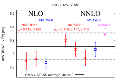
Figure 37: The total cross-sections for $W^{+}$, $W^{-}$ and $Z^{0}$ production at the LHC 7 TeV and their ratios $\sigma(W^{+}+W^{-})/\sigma(Z^{0})$ and $\sigma(W^{+})/\sigma(W^{-})$. Predictions are shown for the same PDF sets and values of $\alpha_{s}$ shown in Fig. 36, and compared to the ATLAS and CMS data summarized in Table 9, shown as a dashed band. Uncertainties shown are one sigma for absolute cross-sections, and 68% confidence levels for cross-section ratios.

A closely related recent measurement by CMS [81] is the ratio of $t\bar{t}$ and $Z$ cross-sections. We have computed predictions for this observable using the VRAP code [53] together with HATHOR, for the same PDF sets and settings. At NNLO this ratio is only weakly dependent on the value of $\alpha_{s}$. Results are also shown in Fig. 36 and compared to the CMS measurement, again shown as a dashed band. The conclusions are similar.

Finally, we consider the total cross-sections for electroweak gauge boson production and their ratios at the LHC. We have computed these observables with the VRAP code [53], within the narrow-width approximation (including the $\gamma^{*}$ contribution to gauge boson production). Results are collected in Fig. 37. As for the case of top production, we show NNPDF2.1 at NLO and NNLO, using our preferred value $\alpha_{s}=0.119$, and also compare NNPDF2.1 with MSTW08 at NLO and NNLO, and ABKM09 at NNLO, using their preferred values of $\alpha_{s}$. Again, we have averaged the most updated CMS [86] and ATLAS [87] results for these observables, assuming they are uncorrelated. The individual ATLAS and CMS results, corresponding to an integrated luminosity of $36$ pb^-1, together with their average are summarized in Table 9. The results are shown as dashed bands on the plots. Note that for cross-section ratios the uncertainty shown is computed as a 68% confidence level, because we have verified that the distribution of results can be markedly non-gaussian.

	ATLAS	CMS	Average
$\sigma\left(W^{+}\right)B\left(l^{+}\nu\right)$ (nb)	$6.26\pm 0.32$	$6.02\pm 0.26$	$6.11\pm 0.20$
$\sigma\left(W^{-}\right)B\left(l^{-}\nu\right)$ (nb)	$4.15\pm 0.21$	$4.26\pm 0.19$	$4.21\pm 0.14$
$\sigma\left(Z^{0}\right)B\left(l^{+}l^{-}\right)$ (nb)	$0.945\pm 0.051$	$0.975\pm 0.044$	$0.962\pm 0.033$
$\sigma\left(W^{+}+W^{-}\right)B\left(l\nu\right)/\sigma\left(Z^{0}\right)B\left(l^{+}l^{-}\right)$	$10.91\pm 0.28$	$10.54\pm 0.19$	$10.65\pm 0.16$
$\sigma\left(W^{+}\right)/\sigma\left(W^{-}\right)$	-	$1.421\pm 0.034$	$1.421\pm 0.034$

Table 9: Recent results from CMS at ATLAS for the total cross-sections for $W^{+}$, $W^{-}$ and $Z^{0}$ production and their ratios, obtained with an integrated luminosity of $\sim 36$ pb^-1, together with their average. The average has been obtained assuming the two measurements to be completely uncorrelated.

The dependence on $\alpha_{s}$ is weaker for these processes, which are quark-dominated, independent of the strong coupling at Born level, and affected by smaller NNLO corrections. However, the dependence of the predictions on the perturbative order is still not negligible. Differences between PDF sets are also less significant, except for the $W^{+}/W^{-}$ cross-section ratio which is a very sensitive probe of the quark flavor decomposition. The general conclusions are similar to those from top production: the LHC data (in particular the $W$ cross-section ratio) already show some discrimination between PDFs. Moreover, for some of these standard candle observables the LHC data may be able to discriminate between NLO and NNLO.

As a general conclusion of this first pehnomenological study, we note that the pattern of comparison between PDF sets is essentially unchanged when going from NLO to NNLO. Therefore, the arguments supporting the PDF4LHC recommendation [77] (and specifically its use in the computation of Higgs exclusion limits [76]) apply equally at NLO and NNLO.

9 Accuracy of the NNLO PDF determination

The NNLO PDF determination is based on the most accurate available theory. It is therefore worth discussing the dependence of results on the main sources of uncertainty. As shown in detail in our previous studies Ref. [6, 62], the main factor which drives PDF uncertainties is the underlying dataset. Also important are the values of the QCD parameters used in the PDF extraction, primarily the value of the strong coupling $\alpha_{s}$, but also of the quark masses: their impact is sometimes comparable to that of the data, in that the uncertainty due to their variation is similar to the PDF uncertainty when they are kept fixed [74, 80, 8, 48]. Here we study both aspects: first, the dependence of PDFs on parameters (specifically $\alpha_{s}$), by repeating the NNPDF2.1 NNLO determination as the underlying parameters are varied, and then the dependence on the size of the dataset by repeating the NNPDF2.1 NNLO determination with various subsets of the global dataset. Theoretical uncertainties will not be studied here: as we argued in Sect. 7, at NNLO the uncertainty related to higher order corrections (as might be estimated by renormalization and factorization scale variation) is usually subdominant, as are those related to the treatment of heavy quarks [48].

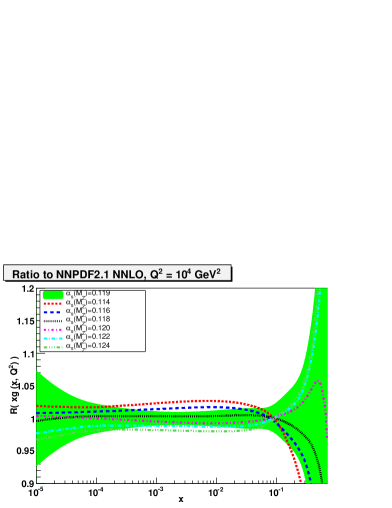
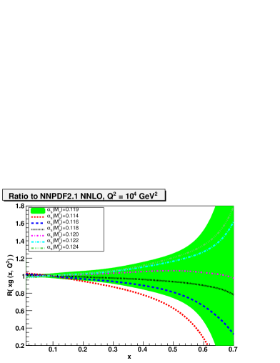
Figure 38: Comparison of NNPDF2.1 NNLO sets with different values of the strong coupling, shown as ratios to reference set with $\alpha_{s}=0.119$ at $Q^{2}=10^{4}$ GeV²: gluon at small and large $x$ (top), triplet at large $x$ and singlet at small $x$ (bottom). To improve readability PDF uncertainties are only shown for the $\alpha_{s}=0.119$ set.

9.1 Dependence on $\alpha_{s}\left(M_{Z}\right)$

In order to determine the dependence of PDFs on the value of $\alpha_{s}$ we have repeated the NNPDF2.1 NNLO determination as $\alpha_{s}$ is varied: we provide sets with $\alpha_{s}\left(M_{Z}\right)$ in the range from 0.114 to 0.124 in steps of 0.001, each including $N_{\rm rep}=100$ PDF replicas. Results for the gluon, the quark singlet and isospin triplet are displayed in Fig. 38, where the ratio of the central PDFs for each value of $\alpha_{s}$ to the default $\alpha_{s}\left(M_{Z}\right)=0.119$ set is shown, and compared to the PDF uncertainty on the central set. Results are qualitatively similar to their NLO counterparts of Ref. [74]: the PDF which is most sensitive to the choice of value of $\alpha_{s}$ is the gluon, which is mostly determined by scaling violations.

Figure 39: Same as Fig. 35, but for NNPDF2.1 NNLO sets with different values of $\alpha_{s}(M_{Z})$. Results are shown as ratios to the NNPDF2.1 NNLO reference with $\alpha_{s}(M_{Z})=0.119$.

As an illustration of the phenomenological impact of the choice of $\alpha_{s}$, in Fig. 39 we present results for the NNLO Higgs cross-section from gluon-gluon fusion (same as Fig. 35) computed using these PDF sets with varying $\alpha_{s}$, again normalized to the central prediction. The dependence on $\alpha_{s}$ of this observable is quite strong, both because it is quadratic in the gluon, and also because it starts at ${\mathcal{O}}(\alpha_{s}^{2})$, and it undergoes NLO corrections which are as large as the LO contribution, and NNLO corrections which are about half of the LO (see Ref. [80, 49] for detailed studies of the relative size of PDF and $\alpha_{s}$ uncertainties on this process).

Finally, in order to study the dependence on the value of the heavy quark masses, we have also produced PDF sets with $m_{c}=1.5,~{}1.6$ and $1.7$ GeV (in addition to the default $m_{c}=\sqrt{2}$ GeV), and with $m_{b}=4.25,~{}4.5,~{}5.0$ and $5.25$ GeV (in addition to the default $m_{b}=4.75$ GeV). The dependence of PDFs on the heavy quark masses is similar to that observed at NLO and discussed in Ref. [8].

9.2 Dependence on the dataset

We now turn to the dependence of PDFs and their uncertainties on the underlying dataset. This dependence is relevant in that one may think that even though a wider dataset always carries more information, smaller datasets may be more consistent (from either the experimental or theoretical point of view), and thus perhaps more reliable. It is thus important to understand what is the price that one pays for this putative improved consistency.

To this purpose, we have constructed four new PDF sets, each based on a subset of the full NNPDF2.1 NNLO dataset, but using exactly the same methodology. The possibility of obtaining reliable PDFs from datasets of widely varying size (more than a factor three, in our case) without having to modify any aspect of the methodology (and in particular without having to change the parametrization, see Ref. [88]) is an advantage of the NNPDF approach, since it allows a meaningful comparison of uncertainties. Each of these PDF sets is made available through the standard LHAPDF interface, and each so far as it goes is as good as the default one, the only difference between them being the smaller amount of experimental information that goes into them.

Experiment	Global	HERA–only	DIS–only	DIS+DY	Collider–only
$N_{\rm dat}$	3357	834	2783	3171	1090
Total	1.16	1.07	1.15	1.18	1.02
NMC-pd	0.93	[13.15]	0.88	0.94	[3.43]
NMC	1.63	[1.91]	1.69	1.69	[2.06]
SLAC	1.01	[3.17]	0.97	1.03	[1.23]
BCDMS	1.32	[2.15]	1.28	1.30	[2.22]
HERAI-AV	1.10	1.05	1.09	1.09	1.06
CHORUS	1.12	[2.63]	1.08	1.13	[1.74]
FLH108	1.26	1.32	1.27	1.26	1.26
NTVDMN	0.49	[60.51]	0.45	0.54	[23.02]
ZEUS-H2	1.31	1.21	1.26	1.28	1.30
ZEUSF2C	0.88	0.77	0.86	0.88	0.75
H1F2C	1.46	1.30	1.47	1.50	1.24
DYE605	0.81	[9.06]	[6.86]	0.82	[1.34]
DYE866	1.32	[12.41]	[2.70]	1.32	[5.76]
CDFWASY	1.65	[7.71]	[13.94]	1.64	1.07
CDFZRAP	2.12	[3.74]	[2.15]	1.91	1.22
D0ZRAP	0.67	[1.11]	[0.67]	0.65	0.61
CDFR2KT	0.74	[1.15]	[0.99]	[1.25]	0.64
D0R2CON	0.82	[1.28]	[0.88]	[1.03]	0.83

Table 10: Quality of the fit for NNLO PDF sets based on datasets of varying size. The total number of data points is given in the first row, followed by the $\chi^{2}$ normalized to the number of data points both for the total fitted set and for each of the individual experiments. The $\chi^{2}$ values for experiments which are not fitted are also shown in square brackets.

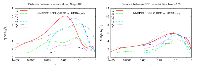
Figure 40: Distances between central values (left) and uncertainties (right) for PDFs in the HERA-only and default NNPDF2.1 NNLO fits. All distances are computed from sets of $N_{\rm rep}=100$ replicas.

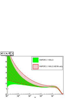
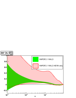
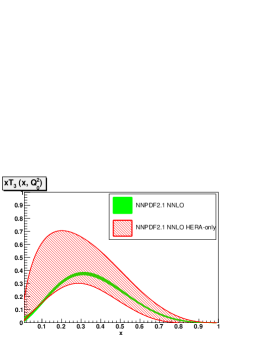
Figure 41: Comparison of NNPDF2.1 NNLO singlet, total strangeness and isotriplet PDFs in the global and in the HERA-only fits.

In particular the fits that we discuss in this section are, in order of increasing complexity:

• HERA data only. This determination exploits a maximally consistent set of data: the combined HERA-I inclusive data, the H1 and ZEUS $F_{2}^{c}$ data and the ZEUS HERA-II data. PDFs based on this dataset have also been determined and published by the HERAPDF group [28].

• Deep-inelastic scattering (DIS) only. This determination does not include hadron-hadron data, which one may perhaps consider theoretically or experimentally less clean than lepton-hadron data.

• Deep-inelastic scattering and Drell-Yan (DIS+DY) only. This determination is in principle the only truly NNLO one, as it excludes jet data, for which only approximate NNLO matrix elements are known. In order to better understand the relevance of approximate NNLO jet corrections, we will also construct a set which only differs from the default one by setting to zero the approximate NNLO terms in jet matrix elements.

• Lepton and hadron collider data only. This determination excludes fixed-target data, which are less clean, both because of the lower energy and because a sizable fraction of them (in particular, all the neutrino DIS data) are obtained using nuclear targets. This determination is of greater complexity than DIS+DY, despite having a smaller number of datapoints, because it also includes jet data.

In each case, a set of $N_{\rm rep}=100$ PDF replicas has been constructed. The NLO counterparts of the DIS and DIS+DY PDF determinations were discussed in Ref. [6] and are available from LHAPDF both for NNPDF2.0 and NNPDF2.1; the HERA-only NLO PDFs were briefly discussed in Ref. [89]; collider-only PDFs are presented here for the first time.

The total $\chi^{2}$ and that of the individual experiments for each of these PDF fits are shown in Table 10, along with the number of data in each reduced dataset, and compared to those of the default NNPDF2.1 fit. In each case, the $\chi^{2}$ of experiments not included in the corresponding fit is also shown, in square brackets.

We now turn to a discussion of these fits, and in particular a comparison between each of them, the default NNPDF2.1, and the fit with immediately greater complexity, in order to assess the impact of individual data. These comparisons are based on the computation of distances (defined as in Appendix A of Ref. [6]) between PDFs in the two sets which are being compared, bearing in mind that $d\sim 1$ means statistical equivalence (the data added have no impact on the given PDF), while $1<d\mathrel{\hbox to0.0pt{\lower 4.0pt\hbox{\hskip 1.0pt$\sim$}\hss}\raise 1.0pt\hbox{$<$}}7$ (for $N_{\rm rep}=100$ replicas) means statistical inequivalence but compatibility at the one sigma level (the data added do have an impact, but only at the one sigma level). Some of the pairs of PDFs with the largest distances will also be compared directly.

The HERA-only PDF set is subject to the limitation that charged-current DIS data are enough to determine at most four independent linear combinations of quark PDFs (see e.g. Ref. [90]), hence strangeness in this set is entirely uncertain — in the HERAPDF [28] set an independent parametrization is only provided for the combinations $d+s$ and $\bar{d}+\bar{s}$, but not separately for strangeness. Indeed, for this fit the quality of the fit to NuTeV dimuon data is extremely poor. This set also provides a poor description of all datasets which are sensitive to the singlet-triplet separation (such as fixed-target DIS and DY data) to the light sea decomposition (such as $W$ production data) and, to a lesser extent, the valence-sea separation (such as neutrino data). The description of the jet data is also of marginal quality.

Figure 42: Distances between central values (left) and uncertainties (right) for PDFs in the DIS-only and default NNPDF2.1 NNLO fits. All distances are computed from sets of $N_{\rm rep}=100$ replicas.

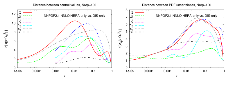
Figure 43: Distances between central values (left) and uncertainties (right) for PDFs in the HERA-only and DIS-only NNPDF2.1 NNLO fits. All distances are computed from sets of $N_{\rm rep}=100$ replicas.

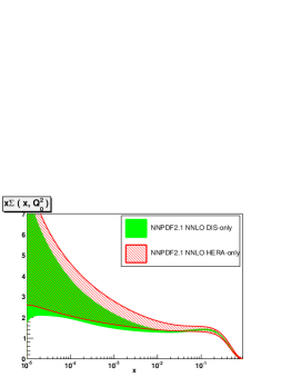
Figure 44: Comparison of NNPDF2.1 NNLO singlet, total strangeness and total valence PDFs in the DIS-only and in the HERA-only fits.

The distances between uncertainties (see Fig. 40) for this fit and the default are largest for the triplet, strangeness, sea asymmetry, and valence. The distance between central values remains large for triplet and strangeness, but it is yet larger for the singlet and gluon: the large shifts in strangeness and triplet are accompanied by a corresponding increase in their uncertainty, while the increase in the uncertainty of the singlet and gluon is more moderate, so the change in central value ends up being statistically more significant, as can be clearly seen in the direct PDF comparison of Fig. 41. All PDFs remain compatible with those of the global fit at the level of 90% confidence level, but the deviation of singlet and gluon is greater than one sigma. Phenomenology based on this PDF set is necessarily very uncertain in any contribution which depends on strangeness, as cross-sections using HERA-only PDF sets have a theoretical uncertainty of order of the size of the strange contribution, which for instance for $W$ and $Z$ production at the LHC is of order 15-25% of the total cross-section [91]. This uncertainty cannot be reduced regardless of the accuracy of the HERA data that go into the PDF determination.

The most severe problems of the HERA-only fit disappear in the DIS-only fit, which thanks to the presence of data with neutrino beams or deuterium targets, achieves reasonably accurate flavor decomposition: indeed, distances between strangeness, valence and light sea asymmetry determined in this fit and those of the global fit, shown in Fig. 42, are rather smaller than one sigma (though uncertainties are still significantly larger), and the singlet and gluon are now in near-perfect agreement with those of the global fit, with only the gluon showing a deviation at the half-sigma level in the large $x$ region. The improvement in accuracy in the flavour decomposition over the HERA-only fit is clear both in the distances between the uncertainties in these two fits (see Fig. 43), and directly comparing PDFs for which the improvement is most dramatic: singlet, strangeness, and valence (Fig. 44). The triplet distribution also shows a significant decrease in uncertainty, but around the valence peak it only agrees with that of the global fit at the 90% confidence level: this may suggest some tension between deuterium DIS and hadron collider data (as has been discussed elsewhere [7, 14]), though it could also be a statistical fluctuation.

As a consequence of all this, the quality of the agreement of the DIS-only PDFs with all Drell-Yan data shown in Table 10 (specifically $W$ and $Z$ production data) remains poor (at the level of many units of $\chi^{2}$), thus showing that a DIS-only PDF fit is not adequate for precision hadron collider phenomenology. On the other hand, it is interesting to observe that the gluon distribution determined by DIS scaling violations is in good agreement with that of the global fit, even in the large $x$ region where jet data have an impact on its uncertainty. Even though the gluon uncertainty at large $x$ is rather smaller in the global fit, the central value agrees at the half sigma level, and indeed the quality of the fit to jet data provided by the DIS-only fit is quite good, though of course not as good as when these data are also fitted. It is interesting to observe that other PDF fits based on reduced datasets (such as HERAPDF or ABKM) do not seem [49] to provide an equally good fit to jet data, presumably because of their less flexible PDF parametrization.

Figure 45: Distances between central values (left) and uncertainties (right) for PDFs in the DIS+DY and default NNPDF2.1 NNLO fits. All distances are computed from sets of $N_{\rm rep}=100$ replicas.

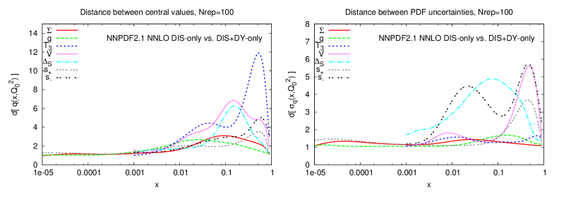
Figure 46: Distances between central values (left) and uncertainties (right) for PDFs in the DIS-only and DIS+DY NNPDF2.1 NNLO fits. All distances are computed from sets of $N_{\rm rep}=100$ replicas.

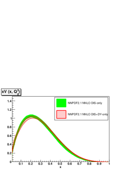
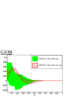
Figure 47: Comparison of NNPDF2.1 NNLO isotriplet, total valence and sea asymmetry PDFs in the DIS-only and in the DIS+DY fits.

Based on this, we expect the DIS+DY fit to be quite close to the default global fit. This expectation is borne out by the plot of the distance between these two fits, Fig. 45. In fact, almost all PDFs in this pair of fits are statistically equivalent. In comparison to the DIS-only fit (Fig. 46), the addition of the Drell-Yan data has a significant impact on all individual quark flavours, reducing the uncertainties of the flavour decomposition, as can also be seen by directly comparing PDFs (Fig. 47).

Figure 48: Distances between central values (left) and uncertainties (right) for PDFs in the default NNPDF2.1 NNLO fit when approximate NNLO jet matrix elements are switched off. All distances are computed from sets of $N_{\rm rep}=100$ replicas.

The only significant impact of jet data is on the gluon at large $x$ whose central value shifts by about half a sigma with a corresponding reduction in uncertainty when going from the DIS+DY to the global fit, also leading to a slight shift of the singlet and valence distributions.

Because of all this, one may wonder whether it might be advantageous to use the DIS+DY fit as the default global NNLO fit, given that the NNLO jet matrix elements are only approximate. To address this issue, we have produced a NNLO fit in which the jet matrix elements are computed at NLO, everything else being as in the NNLO global fit. Distances between this PDF set and the default are displayed in Fig. 48. These distances are all smaller than the distances of Fig. 45 between the reference and DIS+DY fits. Hence, the impact of NNLO corrections to the matrix elements is negligible in comparison to the impact of the jet data (however moderate this be). If one reasonably assumes that the difference between exact and approximate NNLO matrix elements is smaller, or at least not much larger, than the distance between NLO and approximate NNLO, one must conclude that there is no advantage in downgrading to the DIS+DY determination. Thus, the fit with jets at approximate NNLO (i.e. the NNPDF2.1 NNLO default) provides the most accurate PDF determination.

Figure 49: Distances between central values (left) and uncertainties (right) for PDFs in the collider-only and default NNPDF2.1 NNLO fits. All distances are computed from sets of $N_{\rm rep}=100$ replicas.

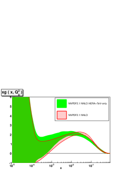
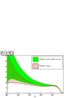
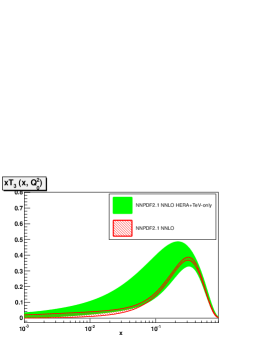
Figure 50: Comparison of NNPDF2.1 NNLO gluon, singlet and triplet PDFs in the collider-only and reference fits.

The last PDF determination that we consider is based on a fit to collider data only. To be precise, we use the same datasets as in the HERA–only fits supplemented by the Tevatron weak-boson production and inclusive jet production data. The quality of the global fit in this case, with $\chi^{2}=1.02$, is significantly better than that of the default global fit: this supports the idea that a collider-only dataset might be more consistent than one which also includes fixed-target data.

However, the distances between the collider-only and global PDFs (Fig. 49) show that they are far from being equivalent: in fact almost all the PDFs show a shift at the one sigma level, with uncertainties significantly larger in the collider-only fit. Correspondingly, the quality of the fit of the collider-only PDFs to the fixed target data is generally poor, especially for deuterium data (such as NMC-pd or DYE866), which control the up-down separation, and the dimuon data (which control strangeness). These increased uncertainties end up contaminating also the singlet and gluon PDFs, as shown by the distance computation and by direct PDF comparison (Fig. 50). Hence, we must conclude that a collider-only fit at present does not provide competitive accuracy for phenomenology due to its extremely poor determination of strangeness and light quark asymmetry, and rather poor determination of valence, triplet and even singlet PDFs. This situation might improve with forthcoming HERA-II and LHC data, so the collider-only fit remains an appealing possibility for the future.

10 Conclusions

The family of NNPDF2.1 PDF determinations — including the NLO set of Ref. [8] and the NNLO and LO sets presented here — provides arguably the most accurate available PDF determination: it is based on a wider dataset than ABKM09 [65] or HERAPDF [28], unlike CT10 [14] it also includes NNLO PDFs, and it is based on a more up-to-date dataset and treatment of uncertainties than MSTW08 [13] (in particular it uses the combined HERA-I data, and correlated uncertainties for all the experiments which supply them). Of course, this is in part due to it being the most recent PDF set, and updates from the other PDF fitting groups are to be expected in the future. However, the NNPDF set is unique in that it is based on a methodology which has been demonstrated [62, 7] to lead to PDFs and uncertainties which behave in a statistically consistent way and minimize parametrization bias.

In Ref. [90] it was proposed that an ideal parton set should satisfy a set of general requirements: NNPDF2.1 now satisfies essentially all of them. Its only shortcoming is that, like all other parton sets to date, it does not include an estimate of the uncertainty related to the truncation of the perturbative expansion (as given for instance by performing renormalization and factorization scale variation). However this is only a problem at NNLO, since at LO and NLO the availability of a higher-order set already provides this information. Furthermore there is every indication that at NNLO the theoretical uncertainty is small compared to the data uncertainties.

With the most relevant methodological and conceptual issues now solved, the emphasis now shifts to making an optimal use of the data which have started to flow so copiously from the LHC experiments.

 

All the NNPDF2.1 NNLO and LO PDF sets that have been discussed in this work are available from the NNPDF web site,

http://sophia.ecm.ub.es/nnpdf 

and through the LHAPDF interface [63] from v.5.8.6-beta onwards. The older NNPDF2.1 NLO PDF sets (called simply NNPDF2.1 on LHAPDF), described in detail in Ref. [8], remain unchanged.

Specifically, the new PDF sets that have been produced in the present analysis and are available in LHAPDF are the following:

• The reference NNPDF2.1 NNLO sets, sets of $N_{\rm rep}=100$ and 1000 replicas:
  NNPDF21_nnlo_100.LHgrid and NNPDF21_nnlo_1000.LHgrid.

• NNPDF2.1 NNLO sets of $N_{\rm rep}=100$ replicas with $\alpha_{s}$ varied from 0.114 to 0.124 with steps of $\delta\alpha_{s}=0.001$:
  NNPDF21_nnlo_as_0114_100.LHgrid, $\ldots$, NNPDF21_nnlo_as_0124_100.LHgrid.

• NNPDF2.1 NNLO sets of $N_{\rm rep}=100$ replicas with $m_{c}$ varied:
  NNPDF21_nnlo_mc_15_100.LHgrid, NNPDF21_nnlo_mc_16_100.LHgrid,
  NNPDF21_nnlo_mc_17_100.LHgrid.

• NNPDF2.1 NNLO sets of $N_{\rm rep}=100$ replicas with $m_{b}$ varied:
  NNPDF21_nnlo_mb_425_100.LHgrid, NNPDF21_nnlo_mb_45_100.LHgrid,
  NNPDF21_nnlo_mb_50_100.LHgrid, NNPDF21_nnlo_mb_525_100.LHgrid.

• The NNPDF2.1 NNLO PDF sets based on reduced datasets:
  NNPDF21_dis_100.LHgrid, NNPDF21_dis+dy_100.LHgrid,
  NNPDF21_heraonly_100.LHgrid, NNPDF21_collider_100.LHgrid.

• The reference NNPDF2.1 LO sets, sets of $N_{\rm rep}=100$, for alphas=0.119 and 0.130:
  NNPDF21_lo_as_0119_100.LHgrid and NNPDF21_lo_as_0130_100.LHgrid.

• The NNPDF2.1 LO* sets, without the momentum sum rule imposed, sets of $N_{\rm rep}=100$, for alphas=0.119 and 0.130:
  NNPDF21_lostar_as_0119_100.LHgrid and NNPDF21_lostar_as_0130_100.LHgrid.

 

Acknowledgments

We are grateful to Lance Dixon for correspondence on the VRAP code, to Frank Petriello for help with DYrap and to Marco Bonvini for help with the treatment of fixed-target Drell-Yan data. We thank Kevin Einsweiler, Ronan McNulty, Frank–Peter Schilling and Michael Schmitt for assistance with LHC data. We also acknowledge discussions with A. Accardi, J. Andersen, P. Nadolsky, F. Olness, R. Thorne, A. Vicini and G. Watt. We afe grateful to G. Watt for pointing out an error in Fig. 34 and to G. Salam for comments on the preprint version of this paper. M.U. is supported by the Bundesministerium für Bildung and Forschung (BmBF) of the Federal Republic of Germany (project code 05H09PAE). This work was partly supported by the Spanish MEC FIS2007-60350 grant. We would like to acknowledge the use of the computing resources provided by the Black Forest Grid Initiative in Freiburg and by the Edinburgh Compute and Data Facility (ECDF) (http://www.ecdf.ed.ac.uk/). The ECDF is partially supported by the eDIKT initiative (http://www.edikt.org.uk).

Appendix A Heavy quark coefficient functions to $\mathcal{O}\left(\alpha_{s}^{2}\right)$ in Mellin space

In this Appendix we provide expressions for the Mellin transforms of the $\mathcal{O}\left(\alpha_{s}^{2}\right)$ massive heavy quark coefficient functions in the $Q^{2}\to\infty$ limit. These asymptotic coefficient functions were first computed long in Ref. [92] in $x$–space. Their Mellin transforms have been given in Refs. [103, 104], and will be rederived here in a form which is suitable for our purposes.

In order to perform the Mellin transform of the $x$–space FFN heavy quark coefficient functions of Ref. [92] it is convenient to rewrite them in terms of independent Mellin integrals, which we can then tabulate.

Following the notation introduced in Ref. [92], we first consider the gluon coefficient function for $F_{L}$. The corresponding Mellin transform can be written as

$$H_{L,g}^{(2)}\left(N,{{Q^{2}}\over{m^{2}}},{{\mu^{2}}\over{m^{2}}}\right)=4T_{f}\left[C_{L,g}^{\rm const}(N)+C_{L,g}^{Q}(N)\ln{{Q^{2}}\over{m^{2}}}-C_{L,g}^{\mu}(N)\ln{{\mu^{2}}\over{m^{2}}}\right].$$ (9)

The coefficient function has been separated into three terms: a $Q^{2}$–independent term $C^{\rm const}(N)$, a collinear log term $C^{Q}(N)$, and a scale variation term $C^{\mu}(N)$. A similar decomposition will be performed for all coefficient functions.

The individual terms are:

$$\begin{array}[]{rcl}C_{L,g}^{\rm const}&=C_{F}&\displaystyle\big{[}\hbox{${{16}\over{15}}$}A_{10}^{(-2)}-\hbox{${{16}\over{3}}$}A_{10}^{(1)}+\hbox{${{32}\over{5}}$}A_{10}^{(3)}+8A_{8}^{(1)}+8A_{6}^{(1)}-\hbox{${{16}\over{3}}$}A_{3}^{(1)}-\hbox{${{16}\over{5}}$}A_{3}^{(3)}\\ &&\displaystyle-\zeta(2)\big{(}\hbox{${{16}\over{3}}$}A_{1}^{(1)}-\hbox{${{32}\over{5}}$}A_{1}^{(3)}\big{)}+4A_{4}^{(0)}+12A_{4}^{(1)}-16A_{4}^{(2)}-\hbox{${{16}\over{15}}$}A_{2}^{(-1)}\\ &&\displaystyle-\hbox{${{52}\over{15}}$}A_{2}^{(0)}-\hbox{${{104}\over{5}}$}A_{2}^{(1)}+\hbox{${{48}\over{5}}$}A_{2}^{(2)}+\hbox{${{16}\over{15}}$}A_{1}^{(-1)}-\hbox{${{64}\over{15}}$}A_{1}^{(0)}-\hbox{${{152}\over{5}}$}A_{1}^{(1)}+\hbox{${{168}\over{5}}$}A_{1}^{(2)}\big{]}\\ &+C_{A}&\displaystyle\big{[}16A_{10}^{(1)}+16A_{10}^{(2)}-32A_{8}^{(1)}+16\zeta(2)A_{1}^{(2)}-48A_{6}^{(1)}+16A_{6}^{(2)}\\ &&\displaystyle+8A_{5}^{(1)}-8A_{5}^{(2)}+24A_{3}^{(1)}+\hbox{${{8}\over{3}}$}A_{4}^{(-1)}-8A_{4}^{(0)}-72A_{4}^{(1)}+\hbox{${{232}\over{3}}$}A_{4}^{(2)}\\ &&\displaystyle+8A_{2}^{(0)}+64A_{2}^{(1)}-104A_{2}^{(2)}-\hbox{${{8}\over{9}}$}A_{1}^{(-1)}+\hbox{${{8}\over{3}}$}A_{1}^{(0)}+\hbox{${{136}\over{3}}$}A_{1}^{(1)}-\hbox{${{424}\over{9}}$}A_{1}^{(2)}\big{]},\end{array}$$ (10a)

$$\begin{array}[]{rl}C_{L,g}^{Q}&\displaystyle=C_{F}[8A_{2}^{(1)}+4A_{1}^{(0)}+4A_{1}^{(1)}-8A_{1}^{(2)}]\\ &\displaystyle+C_{A}\big{[}16A_{4}^{(1)}-16A_{4}^{(2)}-32A_{2}^{(1)}+\hbox{${{8}\over{3}}$}A_{1}^{(-1)}-8A_{1}^{(0)}-40A_{1}^{(1)}+\hbox{${{136}\over{3}}$}A_{1}^{(2)}\big{]},\end{array}$$ (10b)

$$C_{L,g}^{\mu}=C_{A}\big{[}16A_{4}^{(1)}-16A_{4}^{(2)}-32A_{2}^{(1)}+\hbox{${{8}\over{3}}$}A_{1}^{(-1)}-8A_{1}^{(0)}-40A_{1}^{(1)}+\hbox{${{136}\over{3}}$}A_{1}^{(2)}\big{]},$$ (10c)

where the $A_{N}^{(l)}$ are the independent Mellin integrals

$$A^{(l)}_{n}\equiv A_{n}(N+l).$$ (11)

Those for which we will use closed-form analytic expressions are collected in Tables 11 and 12. Some of these Mellin transforms were already computed in Ref. [93] and are repeated here for completeness. The remainder, for which we will use nymerical approximations, are evaluated at the end of this appendix.

The quark coefficient function for $F_{L}$ can be similarly written as

$$H_{L,q}^{(2)}\left(N,{{Q^{2}}\over{m^{2}}},{{\mu^{2}}\over{m^{2}}}\right)=4T_{f}\left[C_{L,q}^{\rm const}(N)+C_{L,q}^{Q}(N)\ln{{Q^{2}}\over{m^{2}}}-C_{L,q}^{\mu}(N)\ln{{\mu^{2}}\over{m^{2}}}\right],$$ (12)

where

$$\begin{array}[]{rcl}C_{L,q}^{\rm const}&=C_{F}&\displaystyle\big{[}-8A_{8}^{(1)}-8A_{6}^{(1)}+8A_{3}^{(1)}+\hbox{${{8}\over{3}}$}A_{4}^{(-1)}-8A_{4}^{(0)}+\hbox{${{16}\over{3}}$}A_{4}^{(2)}+8A_{2}^{(0)}\\ &&\displaystyle-8A_{2}^{(1)}-16A_{2}^{(2)}-\hbox{${{8}\over{9}}$}A_{1}^{(-1)}+\hbox{${{8}\over{3}}$}A_{1}^{(0)}-\hbox{${{32}\over{3}}$}A_{1}^{(1)}+\hbox{${{80}\over{9}}$}A_{1}^{(2)}\big{]},\end{array}$$ (13a)

$$C_{L,q}^{Q}=C_{L,q}^{\mu}=C_{F}\big{[}-8A_{2}^{(1)}+\hbox{${{8}\over{3}}$}A_{1}^{(-1)}-8A_{1}^{(0)}+\hbox{${{16}\over{3}}$}A_{1}^{(2)}\big{]}.$$ (13b)

Finally, the gluon radiation coefficient function for $F_{L}$ can be written as

$$H_{L,GR}^{(2)}\left(N,{{Q^{2}}\over{m^{2}}},{{\mu^{2}}\over{m^{2}}}\right)=4T_{f}\left[C_{L,GR}^{\rm const}(N)+C_{L,GR}^{Q}(N)\ln{{Q^{2}}\over{m^{2}}}\right],$$ (14)

where

$$C_{L,GR}^{\rm const}=C_{F}\big{[}\hbox{${{4}\over{3}}$}(A_{4}^{(1)}-2A_{2}^{(1)}+A_{1}^{(0)})-\hbox{${{50}\over{9}}$}A_{1}^{(1)}\big{]},$$ (15a)

$$C_{L,GR}^{Q}=C_{F}\hbox{${{4}\over{3}}$}A_{1}^{(1)}.$$ (15b)

Let us now turn to the $F_{2}$ heavy quark coefficient functions. In comparison to the longitudinal structure function, there are extra pieces $C^{2Q}(N)$ and $C^{\mu Q}(N)$ arising from the double collinear logarithm. The gluon coefficient function for $F_{2}$ can be written as

$$\begin{array}[]{rl}\displaystyle H_{2,g}^{(2)}\left(N,{{Q^{2}}\over{m^{2}}},{{\mu^{2}}\over{m^{2}}}\right)&\displaystyle=4T_{f}\bigg{[}C_{2,g}^{\rm const}(N)+C_{2,g}^{2Q}(N)\ln^{2}{{Q^{2}}\over{m^{2}}}+C_{2,g}^{Q}(N)\ln{{Q^{2}}\over{m^{2}}}\\ &\displaystyle\qquad\qquad-C_{2,g}^{\mu}(N)\ln{{\mu^{2}}\over{m^{2}}}-C_{2,g}^{\mu Q}(N)\ln{{\mu^{2}}\over{m^{2}}}\ln{{Q^{2}}\over{m^{2}}}\bigg{]},\end{array}$$ (16)

where

$$\begin{array}[]{rcl}C_{2,g}^{\rm const}&=C_{F}&\displaystyle\big{\{}4\big{[}-2B_{16}^{+}-2\zeta(2)B_{17}^{+}+B_{21}^{+}-\hbox{${{3}\over{2}}$}B_{8}^{+}\big{]}\\ &&\displaystyle+2\big{[}-4B_{15}^{-}-2B_{22}^{-}+12B_{19}^{-}+B_{18}^{-}-\hbox{${{5}\over{2}}$}B_{14}^{-}+2B_{12}^{-}+B_{13}^{-}\\ &&\displaystyle-4B_{20}^{-}+4\zeta(2)B_{2}^{-}-\hbox{${{1}\over{3}}$}B_{11}^{-}+3B_{6}^{-}\big{]}+2\big{(}4A_{15}^{(2)}-2A_{22}^{(2)}+A_{18}^{(2)}\\ &&\displaystyle-\hbox{${{7}\over{2}}$}A_{14}^{(2)}+4A_{12}^{(2)}-A_{13}^{(2)}-4\zeta(2)A_{4}^{(2)}+4A_{23}^{(2)}\\ &&\displaystyle+4\zeta(2)A_{2}^{(2)}-A_{11}^{(2)}+11A_{8}^{(2)}\big{)}+32A_{19}^{(1)}+\zeta(3)(28A_{1}^{(0)}\\ &&\displaystyle-24A_{1}^{(1)}+48A_{1}^{(2)})-28A_{6}^{(1)}+36A_{6}^{(2)}+\hbox{${{4}\over{15}}$}A_{10}^{(-2)}+24A_{10}^{(0)}\\ &&\displaystyle+\hbox{${{32}\over{3}}$}A_{10}^{(1)}+\hbox{${{48}\over{5}}$}A_{10}^{(3)}+\zeta(2)\big{(}12A_{1}^{(0)}-\hbox{${{52}\over{3}}$}A_{1}^{(1)}+26A_{1}^{(2)}+\hbox{${{48}\over{5}}$}A_{1}^{(3)}\big{)}\\ &&\displaystyle-\hbox{${{11}\over{2}}$}A_{5}^{(0)}+22A_{5}^{(1)}-21A_{5}^{(2)}-A_{3}^{(0)}+\hbox{${{2}\over{3}}$}A_{3}^{(1)}-13A_{3}^{(2)}-\hbox{${{24}\over{5}}$}A_{3}^{(3)}\\ &&\displaystyle+7A_{4}^{(0)}-33A_{4}^{(1)}+24A_{4}^{(2)}-\hbox{${{4}\over{15}}$}A_{2}^{(-1)}-\hbox{${{178}\over{15}}$}A_{2}^{(0)}+\hbox{${{34}\over{5}}$}A_{2}^{(1)}\\ &&\displaystyle-\hbox{${{168}\over{5}}$}A_{2}^{(2)}+\hbox{${{4}\over{15}}$}A_{1}^{(-1)}-\hbox{${{226}\over{15}}$}A_{1}^{(0)}+\hbox{${{17}\over{5}}$}A_{1}^{(1)}+\hbox{${{82}\over{5}}$}A_{1}^{(2)}\big{\}}\\ &+C_{A}&\displaystyle\big{\{}4\big{[}C_{24}-C_{25}-C_{26}+\hbox{${{3}\over{4}}$}C_{21}+\hbox{${{3}\over{2}}$}C_{20}\big{]}\\ &&\displaystyle+2\big{[}5(A_{15}^{(0)}+2A_{15}^{(1)})+(A_{16}^{(0)}+2A_{16}^{(1)})-3(A_{19}^{(0)}+2A_{19}^{(1)})+\zeta(2)(A_{17}^{(0)}+2A_{17}^{(1)})\big{]}\\ &&\displaystyle+8(2A_{15}^{(1)}+A_{23}^{(1)})-16A_{22}^{(1)}+2A_{21}^{(2)}-4A_{20}^{(2)}+12A_{14}^{(1)}-4A_{14}^{(2)}\\ &&\displaystyle-2A_{12}^{(0)}-16A_{12}^{(1)}+4A_{12}^{(2)}+4A_{13}^{(0)}+16A_{13}^{(1)}-\zeta(2)(10A_{4}^{(0)}-12A_{4}^{(1)}\\ &&\displaystyle+16A_{4}^{(2)})+\hbox{${{4}\over{3}}$}A_{11}^{(0)}+4A_{11}^{(1)}-\zeta(2)(4A_{2}^{(0)}+40A_{2}^{(1)}-8A_{2}^{(2)})\\ &&\displaystyle-\zeta(3)(3A_{1}^{(0)}+14A_{1}^{(1)}+2A_{1}^{(2)})-\hbox{${{8}\over{3}}$}A_{10}^{(-1)}-12A_{10}^{(0)}+4A_{10}^{(1)}\\ &&\displaystyle+\hbox{${{52}\over{3}}$}A_{10}^{(2)}+\hbox{${{16}\over{3}}$}A_{8}^{(-1)}+5A_{8}^{(0)}-16A_{8}^{(1)}+\hbox{${{20}\over{3}}$}A_{8}^{(2)}\\ &&\displaystyle-\zeta(2)\big{(}8A_{1}^{(-1)}+A_{1}^{(0)}+52A_{1}^{(1)}-\hbox{${{199}\over{3}}$}A_{1}^{(2)}\big{)}+4A_{6}^{(0)}\\ &&\displaystyle-72A_{6}^{(1)}+73A_{6}^{(2)}+\hbox{${{4}\over{3}}$}A_{5}^{(-1)}-\hbox{${{3}\over{2}}$}A_{5}^{(0)}+16A_{5}^{(1)}-\hbox{${{107}\over{6}}$}A_{5}^{(2)}\\ &&\displaystyle+46A_{3}^{(1)}-\hbox{${{57}\over{2}}$}A_{3}^{(2)}+\hbox{${{52}\over{9}}$}A_{4}^{(-1)}-\hbox{${{28}\over{3}}$}A_{4}^{(0)}-\hbox{${{215}\over{3}}$}A_{4}^{(1)}+\hbox{${{749}\over{9}}$}A_{4}^{(2)}+\hbox{${{73}\over{3}}$}A_{2}^{(0)}\\ &&\displaystyle+83A_{2}^{(1)}-\hbox{${{1445}\over{9}}$}A_{2}^{(2)}+\hbox{${{20}\over{9}}$}A_{1}^{(-1)}+\hbox{${{233}\over{18}}$}A_{1}^{(0)}+\hbox{${{65}\over{9}}$}A_{1}^{(1)}-\hbox{${{439}\over{18}}$}A_{1}^{(2)}\big{\}},\end{array}$$

$$\begin{array}[]{rcl}C_{2,g}^{2Q}&=C_{F}&\displaystyle\big{[}2A_{4}^{(0)}-4A_{4}^{(1)}+4A_{4}^{(2)}-A_{2}^{(0)}+2A_{2}^{(1)}-4A_{2}^{(2)}-\hbox{${{1}\over{2}}$}A_{1}^{(0)}+2A_{1}^{(1)}\big{]}\\ &+C_{A}&\displaystyle\big{[}2A_{4}^{(0)}-4A_{4}^{(1)}+4A_{4}^{(2)}+2A_{2}^{(0)}+8A_{2}^{(1)}+\hbox{${{4}\over{3}}$}A_{1}^{(-1)}+A_{1}^{(0)}+8A_{1}^{(1)}\\ &&\displaystyle-\hbox{${{31}\over{3}}$}A_{1}^{(2)}\big{]},\end{array}$$ (17a)

$$\begin{array}[]{rcl}C_{2,g}^{Q}&=C_{F}&\displaystyle[2A_{8}^{(0)}-4A_{8}^{(1)}-(8A_{1}^{(0)}-16A_{1}^{(1)}+16A_{1}^{(2)})\zeta(2)-6A_{6}^{(0)}\\ &&\displaystyle+12A_{6}^{(1)}-16A_{6}^{(2)}+4A_{5}^{(0)}-8A_{5}^{(1)}+8A_{5}^{(2)}+2A_{3}^{(0)}-4A_{3}^{(1)}\\ &&\displaystyle+8A_{3}^{(2)}-7A_{4}^{(0)}+24A_{4}^{(1)}-20A_{4}^{(2)}+2A_{2}^{(0)}-12A_{2}^{(1)}+20A_{2}^{(2)}\\ &&\displaystyle+9A_{1}^{(0)}-17A_{1}^{(1)}+4A_{1}^{(2)}]\\ &+C_{A}&\displaystyle\big{[}-4A_{10}^{(0)}-8A_{10}^{(1)}-8A_{10}^{(2)}+4A_{8}^{(0)}+16A_{8}^{(1)}\\ &&\displaystyle-(4A_{1}^{(0)}+8A_{1}^{(2)})\zeta(2)+24A_{6}^{(1)}-8A_{6}^{(2)}+2A_{5}^{(0)}-4A_{5}^{(1)}\\ &&\displaystyle+4A_{5}^{(2)}-4A_{3}^{(0)}-12A_{3}^{(1)}+\hbox{${{8}\over{3}}$}A_{4}^{(-1)}-2A_{4}^{(0)}+40A_{4}^{(1)}-\hbox{${{134}\over{3}}$}A_{4}^{(2)}\\ &&\displaystyle-48A_{2}^{(1)}+50A_{2}^{(2)}+\hbox{${{52}\over{9}}$}A_{1}^{(-1)}-\hbox{${{55}\over{3}}$}A_{1}^{(0)}-\hbox{${{92}\over{3}}$}A_{1}^{(1)}+\hbox{${{407}\over{9}}$}A_{1}^{(2)}\big{]},\end{array}$$ (17b)

$$\begin{array}[]{rcl}C_{2,g}^{\mu}&=C_{A}&\displaystyle\big{\{}4A_{8}^{(0)}+16A_{8}^{(1)}-(4A_{1}^{(0)}-8A_{1}^{(1)}+8A_{1}^{(2)})\zeta(2)+24A_{6}^{(1)}\\ &&\displaystyle-8A_{6}^{(2)}+4A_{5}^{(0)}-8A_{5}^{(1)}+8A_{5}^{(2)}-2A_{3}^{(0)}-8A_{3}^{(1)}+\hbox{${{8}\over{3}}$}A_{4}^{(-1)}\\ &&\displaystyle-2A_{4}^{(0)}+48A_{4}^{(1)}-\hbox{${{158}\over{3}}$}A_{4}^{(2)}-2A_{2}^{(0)}-64A_{2}^{(1)}\\ &&\displaystyle+\hbox{${{62}\over{3}}$}A_{2}^{(2)}+\hbox{${{4}\over{3}}$}A_{1}^{(-1)}-\hbox{${{43}\over{3}}$}A_{1}^{(0)}-\hbox{${{242}\over{3}}$}A_{1}^{(1)}+\hbox{${{281}\over{3}}$}A_{1}^{(2)}\big{\}},\end{array}$$ (17c)

$$\begin{array}[]{rcl}C_{2,g}^{\mu Q}&=C_{A}&\displaystyle\big{[}4A_{4}^{(0)}-8A_{4}^{(1)}+8A_{4}^{(2)}+4A_{2}^{(0)}+16A_{2}^{(1)}+\hbox{${{8}\over{3}}$}A_{1}^{(-1)}+2A_{1}^{(0)}\\ &&\displaystyle+16A_{1}^{(1)}-\hbox{${{62}\over{3}}$}A_{1}^{(2)}\big{]},\end{array}$$ (17d)

where

$$B^{\pm}_{n}\equiv A_{n}^{(0)}\pm 2A_{n}^{(1)}+A_{n}^{(2)},\qquad C_{n}\equiv A_{n}^{(0)}+2A_{n}^{(1)}+2A_{n}^{(2)}.$$ (18)

The quark coefficient function for $F_{2}$ can be written similarly as

$$\begin{array}[]{rl}\displaystyle H_{2,q}^{(2)}\left(N,{{Q^{2}}\over{m^{2}}},{{\mu^{2}}\over{m^{2}}}\right)&\displaystyle=4T_{f}\bigg{[}C_{2,q}^{\rm const}(N)+C_{2,q}^{2Q}(N)\ln^{2}{{Q^{2}}\over{m^{2}}}+C_{2,q}^{Q}(N)\ln{{Q^{2}}\over{m^{2}}}\\ &\displaystyle\qquad-C_{2,q}^{\mu}(N)\ln{{\mu^{2}}\over{m^{2}}}-C_{2,q}^{\mu Q}(N)\ln{{\mu^{2}}\over{m^{2}}}\ln{{Q^{2}}\over{m^{2}}}\bigg{]},\end{array}$$ (19)

where

$$\begin{array}[]{rcl}C_{2,q}^{\rm const}&=C_{F}&\displaystyle\big{[}8(A_{15}^{(0)}+A_{15}^{(1)})+4(A_{13}^{(0)}+A_{13}^{(1)})+2(A_{14}^{(0)}+A_{14}^{(1)})-4(A_{12}^{(0)}+A_{12}^{(1)})\\ &&\displaystyle-8\zeta(2)(A_{2}^{(0)}+A_{2}^{(1)})+\hbox{${{4}\over{3}}$}(A_{11}^{(0)}+A_{11}^{(1)})-\hbox{${{8}\over{3}}$}A_{10}^{(-1)}-8A_{10}^{(0)}-8A_{10}^{(1)}\\ &&\displaystyle-\hbox{${{8}\over{3}}$}A_{10}^{(2)}+\hbox{${{16}\over{3}}$}A_{8}^{(-1)}+4A_{8}^{(0)}-4A_{8}^{(1)}+\hbox{${{8}\over{3}}$}A_{8}^{(2)}-\zeta(2)\big{(}8A_{1}^{(-1)}+4A_{1}^{(0)}\\ &&\displaystyle+4A_{1}^{(1)}-\hbox{${{16}\over{3}}$}A_{1}^{(2)}\big{)}+8A_{6}^{(2)}+\hbox{${{4}\over{3}}$}A_{5}^{(-1)}+A_{5}^{(0)}-A_{5}^{(1)}-\hbox{${{4}\over{3}}$}A_{5}^{(2)}\\ &&\displaystyle+10A_{3}^{(1)}-4A_{3}^{(2)}+\hbox{${{52}\over{9}}$}A_{4}^{(-1)}-\hbox{${{52}\over{3}}$}A_{4}^{(0)}+\hbox{${{40}\over{3}}$}A_{4}^{(1)}-\hbox{${{16}\over{9}}$}A_{4}^{(2)}+\hbox{${{70}\over{3}}$}A_{2}^{(0)}\\ &&\displaystyle-22A_{2}^{(1)}-\hbox{${{176}\over{9}}$}A_{2}^{(2)}+\hbox{${{20}\over{9}}$}A_{1}^{(-1)}+\hbox{${{76}\over{9}}$}A_{1}^{(0)}-\hbox{${{304}\over{9}}$}A_{1}^{(1)}+\hbox{${{208}\over{9}}$}A_{1}^{(2)}\big{]},\end{array}$$ (20a)

$$\begin{array}[]{rcl}C_{2,q}^{2Q}&=C_{F}&\displaystyle\big{[}2A_{2}^{(0)}+2A_{2}^{(1)}+\hbox{${{4}\over{3}}$}A_{1}^{(-1)}+A_{1}^{(0)}-A_{1}^{(1)}-\hbox{${{4}\over{3}}$}A_{1}^{(2)}\big{]},\end{array}$$ (20b)

$$\begin{array}[]{rcl}C_{2,q}^{Q}&=C_{F}&\displaystyle\big{[}4A_{8}^{(0)}+4A_{8}^{(1)}+4A_{6}^{(0)}+4A_{6}^{(1)}-4A_{3}^{(0)}-4A_{3}^{(1)}+\hbox{${{8}\over{3}}$}A_{4}^{(-1)}\\ &&\displaystyle+2A_{4}^{(0)}-2A_{4}^{(1)}-\hbox{${{8}\over{3}}$}A_{4}^{(2)}+8A_{2}^{(2)}+\hbox{${{52}\over{9}}$}A_{1}^{(-1)}-\hbox{${{52}\over{3}}$}A_{1}^{(0)}\\ &&\displaystyle+\hbox{${{40}\over{3}}$}A_{1}^{(1)}-\hbox{${{16}\over{9}}$}A_{1}^{(2)}\big{]},\end{array}$$ (20c)

$$\begin{array}[]{rcl}C_{2,q}^{\mu}&=C_{F}&\displaystyle\big{\{}4A_{8}^{(0)}+4A_{8}^{(1)}+4A_{6}^{(0)}+4A_{6}^{(1)}-2A_{3}^{(0)}-2A_{3}^{(1)}+\hbox{${{8}\over{3}}$}A_{4}^{(-1)}\\ &&\displaystyle+2A_{4}^{(0)}-2A_{4}^{(1)}-\hbox{${{8}\over{3}}$}A_{4}^{(2)}-2A_{2}^{(0)}-10A_{2}^{(1)}+\hbox{${{8}\over{3}}$}A_{2}^{(2)}+\hbox{${{4}\over{3}}$}A_{1}^{(-1)}\\ &&\displaystyle-\hbox{${{40}\over{3}}$}A_{1}^{(0)}+\hbox{${{4}\over{3}}$}A_{1}^{(1)}+\hbox{${{32}\over{3}}$}A_{1}^{(2)}\big{\}},\end{array}$$ (20d)

$$\begin{array}[]{rcl}C_{2,q}^{\mu Q}&=C_{F}&\displaystyle\big{[}4A_{2}^{(0)}+4A_{2}^{(1)}+\hbox{${{8}\over{3}}$}A_{1}^{(-1)}+2A_{1}^{(0)}-2A_{1}^{(1)}-\hbox{${{8}\over{3}}$}A_{1}^{(2)}\big{]}.\end{array}$$ (20e)

The gluon radiation coefficient function for $F_{2}$ can be written as

$$H_{2,GR}^{(2)}\left(N,{{Q^{2}}\over{m^{2}}},{{\mu^{2}}\over{m^{2}}}\right)=4T_{f}\left[C_{2,GR}^{\rm const}(N)+C_{2,GR}^{2Q}(N)\ln^{2}{{Q^{2}}\over{m^{2}}}+C_{2,GR}^{Q}(N)\ln{{Q^{2}}\over{m^{2}}}\right],$$ (21)

where

$$\begin{array}[]{rcl}C_{2,GR}^{\rm const}&=C_{F}&\displaystyle\big{[}-\hbox{${{2}\over{3}}$}(A_{33}^{(0)}+A_{33}^{(2)})-\hbox{${{2\zeta(2)}\over{3}}$}(2A_{27}^{(0)}-A_{1}^{(0)}-A_{1}^{(1)})-\hbox{${{4}\over{3}}$}(A_{32}^{(0)}+A_{32}^{(2)})\\ &&\displaystyle+\hbox{${{1}\over{3}}$}(2A_{30}^{(0)}-A_{5}^{(0)}-A_{5}^{(1)})+A_{31}^{(0)}+A_{31}^{(2)}-\hbox{${{29}\over{18}}$}(2A_{28}^{(0)}-A_{4}^{(0)}-A_{4}^{(1)})\\ &&\displaystyle+\hbox{${{67}\over{18}}$}(A_{29}^{(0)}+A_{29}^{(2)})+\hbox{${{359}\over{108}}$}(2A_{27}^{(0)}-A_{1}^{(0)}-A_{1}^{(1)})+\hbox{${{1}\over{6}}$}A_{4}^{(0)}+\hbox{${{13}\over{6}}$}A_{4}^{(1)}\\ &&\displaystyle-\hbox{${{1}\over{2}}$}A_{2}^{(0)}-\hbox{${{23}\over{6}}$}A_{2}^{(1)}+\hbox{${{29}\over{36}}$}A_{1}^{(0)}-\hbox{${{295}\over{36}}$}A_{1}^{(1)}+\hbox{${{134\zeta(2)}\over{18}}$}+\hbox{${{265}\over{36}}$}\big{]},\end{array}$$ (22a)

$$C_{2,GR}^{2Q}=C_{F}\big{[}\hbox{${{1}\over{3}}$}(2A_{27}^{(0)}-A_{1}^{(0)}-A_{1}^{(1)})+\hbox{${{1}\over{2}}$}\big{]},$$ (22b)

$$\begin{array}[]{rcl}C_{2,GR}^{Q}&=C_{F}&\displaystyle\big{[}\hbox{${{2}\over{3}}$}(2A_{28}^{(0)}-A_{4}^{(0)}-A_{4}^{(1)})-\hbox{${{29}\over{18}}$}(2A_{27}^{(0)}-A_{1}^{(0)}-A_{1}^{(1)})\\ &&\displaystyle-\hbox{${{4}\over{3}}$}(A_{29}^{(0)}+A_{29}^{(2)})+\hbox{${{1}\over{6}}$}A_{1}^{(0)}+\hbox{${{13}\over{6}}$}A_{1}^{(1)}-\hbox{${{8\zeta(2)}\over{3}}$}-\hbox{${{19}\over{6}}$}\big{]}.\end{array}$$ (22c)

$n$	—$f_{n}(z)$	$A_{n}(N)=\mathbf{M}[f_{n}(z)](N)$
1	—$1$	$\displaystyle{{1}\over{N}}$
2	—$\ln(z)$	$\displaystyle-{{1}\over{N^{2}}}$
3	—$\ln^{2}(z)$	$\displaystyle{{2}\over{N^{3}}}$
4	—$\ln(1-z)$	$\displaystyle-{{S_{1}(N)}\over{N}}$
5	—$\ln^{2}(1-z)$	$\displaystyle{{S_{1}^{2}(N)+S_{2}(N)}\over{N}}$
6	—$\ln(z)\ln(1-z)$	$\displaystyle{{S_{1}(N)}\over{N^{2}}}+{{S_{2}(N)-\zeta(2)}\over{N}}$
8	—$\mbox{Li}_{2}(1-z)$	$\displaystyle-{{S_{2}(N)-\zeta(2)}\over{N}}$
10	—$\mbox{Li}_{2}(-z)+\ln(z)\ln(1+z)$	$\displaystyle-{{\zeta(2)}\over{2N}}-{{1}\over{4N}}\left[S_{2}\left({{N-1}\over{2}}\right)-S_{2}\left({{N}\over{2}}\right)\right]$
11	—$\ln^{3}(z)$	$\displaystyle-{{6}\over{N^{4}}}$
12	—$\ln^{2}(z)\ln(1-z)$	$\displaystyle{{2}\over{N}}\left[\zeta(3)+{{\zeta(2)}\over{N}}-{{S_{1}(N)}\over{N^{2}}}-{{S_{2}(N)}\over{N}}-S_{3}(N)\right]$
13	—$\ln(1-z)\mbox{Li}_{2}(1-z)-\mbox{Li}_{3}(1-z)$	$\displaystyle{{S_{1}(N)S_{2}(N)-\zeta(2)S_{1}(N)+S_{3}(N)-\zeta(3)}\over{N}}$
14	—$\ln(z)\ln^{2}(1-z)$	$\begin{array}[]{l}\displaystyle{{2}\over{N}}\bigg{\{}\zeta(3)+\zeta(2)S_{1}(N)-{{1}\over{2N}}\left[S_{1}^{2}(N)+S_{2}(N)\right]\\ \displaystyle-S_{1}(N)S_{2}(N)-S_{3}(N)\bigg{\}}\end{array}$
15	—$S_{1,2}(1-z)$	$\displaystyle-{{1}\over{N}}\left[S_{3}(N)-\zeta(3)\right]$
17	—$\ln(1+z)$	$\displaystyle{{\ln(2)}\over{N}}+{{1}\over{2N}}\left[S_{1}\left({{N-1}\over{2}}\right)-S_{1}\left({{N}\over{2}}\right)\right]$
18	—$\ln^{3}(1-z)$	$\displaystyle-{{S_{1}^{3}(N)+3S_{1}(N)S_{2}(N)+2S_{3}(N)}\over{N}}$
19	—$\mbox{Li}_{3}(-z)$	$\displaystyle-{{3\zeta(3)}\over{4N}}+{{\zeta(2)}\over{2N^{2}}}-{{\ln(2)}\over{N^{3}}}-{{1}\over{2N^{3}}}\left[S_{1}\left({{N-1}\over{2}}\right)-S_{1}\left({{N}\over{2}}\right)\right]$

Table 11: Elementary Mellin transforms.

$n$	—$f_{n}(z)$	$A_{n}(N)=\mathbf{M}[f(z)](N)$
20	—$\ln(z)\mbox{Li}_{2}(-z)$	$\begin{array}[]{l}\displaystyle-{{1}\over{2N^{2}}}\left[{{2}\over{N}}S_{1}\left({{N-1}\over{2}}\right)+{{1}\over{2}}S_{2}\left({{N-1}\over{2}}\right)+{{4\ln(2)}\over{N}}\right]\\ \displaystyle+{{1}\over{2N^{2}}}\left[{{2}\over{N}}S_{1}\left({{N}\over{2}}\right)+{{1}\over{2}}S_{2}\left({{N}\over{2}}\right)+\zeta(2)\right]\end{array}$
21	—$\ln^{2}(z)\ln(1+z)$	$\begin{array}[]{l}\displaystyle{{1}\over{2N}}\bigg{[}{{2}\over{N^{2}}}S_{1}\left({{N-1}\over{2}}\right)+{{1}\over{N}}S_{2}\left({{N-1}\over{2}}\right)+{{1}\over{2}}S_{3}\left({{N-1}\over{2}}\right)+{{4\ln(2)}\over{N^{2}}}\bigg{]}\\ \displaystyle-{{1}\over{2N}}\bigg{[}{{2}\over{N^{2}}}S_{1}\left({{N}\over{2}}\right)+{{1}\over{N}}S_{2}\left({{N}\over{2}}\right)+{{1}\over{2}}S_{3}\left({{N}\over{2}}\right)\bigg{]}\end{array}$
23	—$\ln(z)\mbox{Li}_{2}(1-z)$	$\displaystyle{{1}\over{N^{2}}}[S_{2}(N)-\zeta(2)]+{{2}\over{N}}[S_{3}(N)-\zeta(3)]$
27	—$\displaystyle\left({{1}\over{1-z}}\right)_{+}$	$-S_{1}(N-1)$
28	—$\displaystyle\left({{\ln(1-z)}\over{1-z}}\right)_{+}$	$\displaystyle{{1}\over{2}}S_{1}^{2}(N-1)+{{1}\over{2}}S_{2}(N-1)$
29	—$\displaystyle{{\ln(z)}\over{1-z}}$	$\displaystyle S_{2}(N-1)-\zeta(2)$
30	—$\displaystyle\left({{\ln^{2}(1-z)}\over{1-z}}\right)_{+}$	$\displaystyle-{{1}\over{3}}S_{1}^{2}(N-1)-S_{1}(N-1)S_{2}(N-1)-{{2}\over{3}}S_{3}(N-1)$
31	—$\displaystyle{{\ln^{2}(z)}\over{1-z}}$	$\displaystyle-2[S_{3}(N-1)-\zeta(3)]$
32	—$\displaystyle{{\ln(z)\ln(1-z)}\over{1-z}}$	$\displaystyle\zeta(3)+\zeta(2)S_{1}(N-1)-S_{1}(N-1)S_{2}(N-1)-S_{3}(N+l-1)$

Table 12: Continuation of Table 11.

In addition to the elementary Mellin transforms listed in Tables 11-12, the coefficient functions contain terms whose Mellin transform is known in closed form, but is expressed in terms of generalized harmonic sums $S_{i_{1},\dots,i_{n}}(N)$. We have evaluated the Mellin transform of these functions through suitable numerical approximations. The $x$–space expression whose Mellin transform will be evaluated in this way are the following:

$$f_{16}(z)=2\mbox{Li}_{2}(-z)\ln(1+z)+\ln(z)\ln^{2}(1+z)+2S_{1,2}(-z),$$ (23a)

$$f_{22}(z)=\mbox{Li}_{3}(1-z),$$ (23b)

$$f_{24}(z)=\mbox{Li}_{3}\left({{1-z}\over{1+z}}\right)-\mbox{Li}_{3}\left(-{{1-z}\over{1+z}}\right),$$ (23c)

$$f_{25}(z)=\ln(z)\ln(1-z)\ln(1+z),$$ (23d)

$$f_{26}(z)=\ln(1-z)\mbox{Li}_{2}(-z),$$ (23e)

$$f_{33}(z)={{\mbox{Li}_{2}(1-z)}\over{1-z}}.$$ (23f)

We will now consider each of these functions in turn.

In order to determine the Mellin transform of Eq. (23a), we use Eq. (32) of Ref. [93], which can be written as

$$\begin{array}[]{rl}\displaystyle A_{16}(N)=\mathbf{M}[f_{16}(z)](N)&=\displaystyle{{1}\over{N}}\mathbf{M}\left[{{z\widetilde{\Phi}(z)}\over{1+z}}\right]-{{1}\over{2N}}\mathbf{M}\left[{{z\ln^{2}(z)}\over{1+z}}\right]\\ \\ &\displaystyle+{{\zeta(2)}\over{N}}\mathbf{M}\left[{{z}\over{1+z}}\right]-{{\zeta(2)\ln(2)}\over{N}}+{{\zeta(3)}\over{4N}}.\end{array}$$ (24)

The last two Mellin transforms are respectively:

$$\mathbf{M}\left[{{z\ln^{2}(z)}\over{1+z}}\right]=-{{1}\over{4}}\left[S_{3}\left({{N-1}\over{2}}\right)-S_{3}\left({{N}\over{2}}\right)\right],$$ (26)

and

$$\mathbf{M}\left[{{z}\over{1+z}}\right]=-{{1}\over{2}}\left[S_{1}\left({{N-1}\over{2}}\right)-S_{1}\left({{N}\over{2}}\right)\right].$$ (27)

The Mellin transform of the term involving the special function $\widetilde{\Phi}(z)$ is given in Ref. [93] in terms of the generalized harmonic sum $S_{1,2}(N)$. To avoid evaluating this directly for complex $N$, we instead rewrite

$${{z\widetilde{\Phi}(z)}\over{1+z}}\cong\sum_{k=1}^{10}a_{k}z^{k}\widetilde{\Phi}(z),$$ (28)

where the values of the coefficients $a_{k}$ are determined by fitting the polynomial $\sum_{k=1}^{10}a_{k}z^{k}$ to the function $z/(1+z)$ on the unit interval. One can then use the Mellin transform of the function $z^{k}\widetilde{\Phi}(z)$, which reads

$$\mathbf{M}[z^{k}\widetilde{\Phi}(z)]={{1}\over{(N+k)^{3}}}+{{1}\over{2(N+k)}}\left[S_{2}\left({{N+k-1}\over{2}}\right)-S_{2}\left({{N+k}\over{2}}\right)\right].$$ (29)

The desired Mellin transform $A_{16}(N)$ is immediately found combining Eqs. (26), (27), (28) and (29).

In order to determine the Mellin transform of Eq. (23b) we use the expansion

$$\mbox{Li}_{3}(z)=\sum_{k=1}^{\infty}{{z^{k}}\over{k^{3}}}.$$ (30)

It follows that

$$A_{22}(N)=\mathbf{M}[f_{22}(z)](N)=\sum_{k=1}^{\infty}{{1}\over{k^{3}}}\int_{0}^{1}z^{N-1}(1-z)^{k}dz,$$ (31)

but

$$\int_{0}^{1}z^{N-1}(1-z)^{k}dz={{\Gamma(N)\Gamma(k+1)}\over{\Gamma(N+k+1)}}={{k!}\over{(N+k)\dots(N+1)N}},$$ (32)

so that

$$A_{22}(N)=\sum_{k=1}^{\infty}{{k!}\over{k^{3}(N+k)\dots(N+1)N}}.$$ (33)

In our implementation we have truncated this series at $k=30$.

Next, we turn to the Mellin transform of Eq. (23c). In this case we fit the function

$$g(z)=(1-z)^{b-1}\sum_{k=0}^{10}c_{k}z^{k}$$ (34)

to the function $f_{24}(z)$. However, one can show that

$$f_{24}(0)=\mbox{Li}_{3}(1)-\mbox{Li}_{3}(-1)=\hbox{${{7}\over{4}}$}\zeta(3)=c_{0},$$ (35)

so that $c_{0}$ is fixed, and we only have to fit

$$g(z)=(1-z)^{b-1}\big{[}\hbox{${{7}\over{4}}$}\zeta(3)+\sum_{k=1}^{10}c_{k}z^{k}\big{]}.$$ (36)

The Mellin transform of Eq. (23c) follows immediately, because

$$\begin{array}[]{rl}\displaystyle A_{24}(N)=\mathbf{M}[f_{24}(z)](N)&=\sum_{k=0}^{10}c_{k}\int_{0}^{1}z^{N+k-1}(1-z)^{b-1}dz\\ &\displaystyle={{\Gamma(N)\Gamma(b)}\over{\Gamma(N+b)}}\sum_{k=0}^{10}c_{k}{{(N+k)\dots(N+1)N}\over{(N+b+l+k)\dots(N+b+l)}}.\end{array}$$ (37)

In order to determine the Mellin transform of Eq. (23d), we use the representation given as Eq. (21) of Ref. [94], in which the function $\ln(1+z)$ is approximated by the polynomial

$$\ln(1+z)\cong\sum_{k=1}^{8}d_{k}z^{k}.$$ (38)

Using also Table 11, we then get

$$\begin{array}[]{c}\displaystyle A_{25}(N)=\mathbf{M}[f_{25}(z)](N)=\sum_{k=1}^{8}d_{k}\mathbf{M}[z^{k}\ln(z)\ln(1-z)]=\\ \\ \displaystyle\sum_{k=1}^{8}d_{k}\left[{{S_{1}(N+k)}\over{(N+k)^{2}}}+{{S_{2}(N+k)-\zeta(2)}\over{N+k}}\right].\end{array}$$ (39)

In order to determine the Mellin transform of Eq. (23e) we use the expansion

$$\mbox{Li}_{2}(-z)=\sum_{k=1}^{\infty}{{(-1)^{k}z^{k}}\over{k^{2}}},$$ (40)

so

$$A_{26}(N)=\mathbf{M}[f_{26}(z)](N)=\sum_{k=1}^{\infty}{{(-1)^{k}}\over{k^{2}}}\mathbf{M}[z^{k}\ln(1-z)]=\sum_{k=1}^{\infty}{{(-1)^{k+1}}\over{k^{2}}}{{S_{1}(N+k)}\over{N+k}}.$$ (41)

In this case we have chosen to truncate the series at $k=100$.

Finally, we determine the Mellin transform of Eq. (23f). In this case we use the geometric series for $1/(1-z)$ so that

$$\begin{array}[]{c}\displaystyle A_{33}(N)\mathbf{M}\left[f_{33}(z)\right](N)=\sum_{k=0}^{\infty}\mathbf{M}[z^{k}\mbox{Li}_{2}(1-z)]=-\sum_{k=0}^{\infty}{{S_{2}(N+k)-\zeta(2)}\over{N+k}}.\end{array}$$ (42)

As in the case above, the series is truncated at $k=100$.

Note that the Mellin transform of the $x$-space coefficient functions involve terms of the form $z^{l}f_{n}(z)$. The Mellin transform $\mathbf{M}[z^{l}f_{n}(z)](N)$ can be obtained from $\mathbf{M}[f_{n}(z)](N)$ using the identity $\mathbf{M}[z^{l}f_{n}(z)](N)=\mathbf{M}[f_{n}(z)](N+l)$. Thus the Mellin transform of any of the terms in Tables 11-12 and also any of the terms Eqs.(23a)-(23f) multiplied by a factor $z^{l}$ can be obtained replacing $N$ with $N+l$.

In conclusion, we have checked our calculation by comparing the inverse Mellin transform of the $N$-space coefficients with the original $x$-space results. We show in Table 13 the accuracy of this comparison for the various coefficient functions. We find excellent accuracy for all coefficients and all values of $x$.

$x$	$\epsilon_{\rm rel}\left(C_{2,g}^{(n_{l},0),2}\right)$	$\epsilon_{\rm rel}\left(C_{2,q}^{(n_{l},0),2}\right)$	$\epsilon_{\rm rel}\left(C_{L,g}^{(n_{l},0),2}\right)$	$\epsilon_{\rm rel}\left(C_{L,q}^{(n_{l},0),2}\right)$
$10^{-7}$	$7\times 10^{-12}$	$4\times 10^{-11}$	$2\times 10^{-10}$	$7\times 10^{-12}$
$10^{-6}$	$3\times 10^{-11}$	$1\times 10^{-11}$	$4\times 10^{-11}$	$3\times 10^{-12}$
$10^{-5}$	$2\times 10^{-12}$	$3\times 10^{-11}$	$4\times 10^{-13}$	$2\times 10^{-12}$
$10^{-4}$	$6\times 10^{-10}$	$1\times 10^{-11}$	$3\times 10^{-11}$	$4\times 10^{-12}$
$10^{-3}$	$6\times 10^{-9}$	$2\times 10^{-12}$	$1\times 10^{-10}$	$2\times 10^{-11}$
$10^{-2}$	$7\times 10^{-8}$	$7\times 10^{-12}$	$2\times 10^{-10}$	$1\times 10^{-11}$
$10^{-1}$	$1\times 10^{-7}$	$4\times 10^{-11}$	$1\times 10^{-11}$	$5\times 10^{-13}$
$3\times 10^{-1}$	$9\times 10^{-7}$	$1\times 10^{-11}$	$1\times 10^{-11}$	$5\times 10^{-13}$
$5\times 10^{-1}$	$4\times 10^{-6}$	$3\times 10^{-11}$	$8\times 10^{-12}$	$1\times 10^{-13}$
$7\times 10^{-1}$	$1\times 10^{-5}$	$9\times 10^{-11}$	$6\times 10^{-12}$	$5\times 10^{-13}$
$9\times 10^{-1}$	$1\times 10^{-5}$	$6\times 10^{-8}$	$7\times 10^{-8}$	$1\times 10^{-8}$

Table 13: Comparison of the inverse Mellin transforms of coefficient functions computed here to the original $x$–space expressions of Ref. [92]: the percentage difference between the original expression and the numerical Mellin inverse is shown in each case.

Appendix B FastKernel implementation of FONLL-C

In this Appendix we discuss the implementation and benchmarking of the FONLL-C neutral current structure functions in the FastKernel framework. At the same time we have implemented and benchmarked FONLL-B, since we expect to perform fits using this scheme in the future.

The implementation of FONLL-B and FONLL-C structure functions in FastKernel requires the $\mathcal{O}\left(\alpha_{s}^{2}\right)$ massive heavy quark coefficient functions as well as their asymptotic $Q^{2}\to\infty$ limit in Mellin space. In Ref. [8] we presented analytic results for the Mellin space $\mathcal{O}\left(\alpha_{s}\right)$ heavy quark coefficient functions for neutral current and charged current scattering (see also Ref. [95] for the latter). For the $\mathcal{O}\left(\alpha_{s}^{2}\right)$ heavy quark coefficient functions in Mellin space we use the parametrization of Ref. [96]. The Mellin transforms in the asymptotic limit as $Q^{2}\to\infty$ have been determined as in Appendix A.

The $\mathcal{O}\left(\alpha_{s}^{2}\right)$ massless coefficient functions were first computed in Refs. [97, 98, 99, 100]. For the implementation in the FastKernel framework we have used the fast Mellin space parametrizations of the exact coefficient functions as given in Refs. [101, 102].

The gluon radiation terms, namely contributions with heavy quarks in the final state but where the struck quark is light, have to be treated with care. As discussed in Ref. [12], the gluon radiation contribution (which first appears at $\mathcal{O}\left(\alpha_{s}^{2}\right)$) is part of the light quark structure functions. We have checked (see Fig. 51) that the size of these terms is very small both for the $F_{2}$ and $F_{L}$ structure functions, typically below 1%.

Figure 51: Percentage difference between the NNLO light quark structure functions $F_{2}$ (left) and $F_{L}$ (right) with and without gluon radiation contributions. From bottom to top the points correspond to scales of $Q^{2}$=4, 10 and 100 GeV² respectively.

Now we turn to the implementation and benchmarking of these results in the FastKernel framework. Benchmarking has been performed by comparing the FastKernel results with the FONLLdis code [12], an $x$-space code that implements all FONLL schemes. In Table 14 we show the results of the benchmark comparison for the $F_{2c}(x,Q^{2})$ and $F_{Lc}(x,Q^{2})$ structure functions in the massive fixed-flavour number scheme at $\mathcal{O}\left(\alpha_{s}^{2}\right)$ for the FONLLdis code and for the FastKernel code. Results are provided at the reference points in the $(x,Q^{2})$ plane and with the settings of the Les Houches heavy quark benchmarks [48]. The accuracy is given as the percentage difference between the FastKernel and FONLLdis calculations. The accuracy is never worse than 1%, which is amply sufficient for our purposes. The accuracy of Table 14 is a little worse than that of its $\mathcal{O}\left(\alpha_{s}\right)$ counterpart, shown as Tables 14-15 of Ref. [8]. This may be due to the fact that the Mellin space parametrizations of the heavy quark coefficient functions that we use [96] are in turn based on a parametrization of the exact $x$-space coefficient functions, while FONLLdis uses the original exact coefficient functions of Ref [105]. This loss of accuracy is negligible for the needs of current phenomenology, but more detailed studies of this issue may be needed in the future when final combined HERA heavy quark structure function data become available.

The same comparisons for the FONLL-B and FONLL-C are presented in Tables 15 and 16 respectively. Comparable accuracy is achieved for these two GM-VFN schemes, again sufficient for our purposes.

	$F_{2c}$ FFNS			$F_{Lc}$ FFNS
$x$	FONLLdis	FastKernel	Accuracy (%)	FONLLdis	FastKernel	Accuracy (%)
$Q^{2}=4$ GeV2
$10^{-5}$	0.24591	0.24244	1.43	0.02215	0.02184	1.41
$10^{-4}$	0.13658	0.13481	1.31	0.01306	0.01283	1.75
$10^{-3}$	0.06384	0.06308	1.20	0.00662	0.00653	1.41
$10^{-2}$	0.02025	0.02007	0.92	0.00238	0.00237	0.38
$Q^{2}=10$ GeV2
$10^{-5}$	0.53701	0.53904	0.38	0.08031	0.08105	0.91
$10^{-4}$	0.29558	0.29550	0.03	0.04611	0.04579	0.71
$10^{-3}$	0.13909	0.13852	0.24	0.02273	0.02254	0.86
$10^{-2}$	0.04689	0.04664	0.10	0.00832	0.00826	0.70
$Q^{2}=100$ GeV2
$10^{-5}$	1.99594	2.00744	0.57	0.44200	0.43976	0.51
$10^{-4}$	1.00912	1.01479	0.56	0.22148	0.21880	1.22
$10^{-3}$	0.43527	0.43410	0.27	0.09487	0.09380	1.14
$10^{-2}$	0.13574	0.13492	0.61	0.03019	0.03002	0.57

Table 14: Benchmark comparisons for the $F_{2c}(x,Q^{2})$ and $F_{Lc}(x,Q^{2})$ structure functions in the FFN scheme at O($\alpha_{s}^{2}$) obtained using the FONLLdis code [12] and the FastKernel code. Results are provided at the benchmark kinematical points in $x,Q^{2}$ and with the settings of the Les Houches heavy quark benchmarks [48]. The accuracy is given as the percentage difference between the FastKernel and FONLLdis [12] calculations.

	$F_{2c}$ FONLL-B			$F_{Lc}$ FONLL-B
$x$	FONLLdis	FastKernel	Accuracy (%)	FONLLdis	FastKernel	Accuracy (%)
$Q^{2}=4$ GeV2
$10^{-5}$	0.24787	0.24858	0.29	0.02519	0.02524	0.21
$10^{-4}$	0.13556	0.13598	0.31	0.01435	0.01435	0.01
$10^{-3}$	0.06360	0.06350	0.15	0.00718	0.00715	0.34
$10^{-2}$	0.02062	0.02051	0.52	0.00258	0.00258	0.08
$Q^{2}=10$ GeV2
$10^{-5}$	0.55100	0.55088	0.02	0.09637	0.09679	0.43
$10^{-4}$	0.30114	0.30150	0.14	0.05229	0.05222	0.14
$10^{-3}$	0.14371	0.14375	0.02	0.02507	0.02499	0.32
$10^{-2}$	0.05012	0.05015	0.01	0.00908	0.00907	0.06
$Q^{2}=100$ GeV2
$10^{-5}$	2.10034	2.08834	0.57	0.48769	0.48716	0.11
$10^{-4}$	1.04510	1.05096	0.56	0.23569	0.23418	0.65
$10^{-3}$	0.45879	0.45916	0.08	0.09923	0.09888	0.35
$10^{-2}$	0.15039	0.15030	0.06	0.03170	0.03174	0.15

Table 15: Same as Table 14 for the FONLL-B GM-VFN scheme.

	$F_{2c}$ FONLL-C			$F_{Lc}$ FONLL-C
$x$	FONLLdis	FastKernel	Accuracy (%)	FONLLdis	FastKernel	Accuracy (%)
$Q^{2}=4$ GeV2
$10^{-5}$	0.27830	0.28163	1.18	0.02468	0.02500	1.30
$10^{-4}$	0.14709	0.14858	1.00	0.01423	0.01441	1.23
$10^{-3}$	0.06556	0.06591	0.52	0.00733	0.00735	0.24
$10^{-2}$	0.02034	0.02034	0.00	0.00281	0.00283	0.74
$Q^{2}=10$ GeV2
$10^{-5}$	0.69412	0.69873	0.66	0.09909	0.10062	1.52
$10^{-4}$	0.34662	0.34911	0.88	0.05520	0.05550	0.52
$10^{-3}$	0.15025	0.15114	0.32	0.02682	0.02699	0.63
$10^{-2}$	0.04986	0.05022	0.13	0.01002	0.01008	0.58
$Q^{2}=100$ GeV2
$10^{-5}$	2.36920	2.37887	0.41	0.47822	0.47994	0.36
$10^{-4}$	1.12695	1.13870	1.03	0.23916	0.23914	0.01
$10^{-3}$	0.47058	0.47317	0.55	0.10262	0.10293	0.30
$10^{-2}$	0.15175	0.15236	0.40	0.03312	0.03327	0.47

Table 16: Same as Table 14 for the FONLL-C GM-VFN scheme.

Appendix C Benchmarking the NNLO PDF evolution

In this appendix we benchmark the accuracy of the NNLO PDF evolution as implemented in the FastKernel framework. The NNLO anomalous dimensions for DGLAP evolution were computed in Refs. [106, 107]. In our code we use the accurate Mellin space parametrizations also provided in Refs. [106, 107].

$x$	$\epsilon_{\rm rel}\left(u_{v}\right)$	$\epsilon_{\rm rel}\left(xd_{v}\right)$	$\epsilon_{\rm rel}\left(L_{-}\right)$	$\epsilon_{\rm rel}\left(L_{+}\right)$	$\epsilon_{\rm rel}\left(s_{+}\right)$	$\epsilon_{\rm rel}\left(g\right)$
$10^{-7}$	$2.5\,10^{-4}$	$2.5\,10^{-4}$	$3.4\,10^{-5}$	$2.7\,10^{-5}$	$4.7\,10^{-5}$	$5.7\,10^{-5}$
$10^{-6}$	$1.5\,10^{-4}$	$1.0\,10^{-4}$	$1.0\,10^{-4}$	$6.1\,10^{-5}$	$5.0\,10^{-5}$	$5.8\,10^{-5}$
$10^{-5}$	$1.7\,10^{-4}$	$1.6\,10^{-4}$	$1.1\,10^{-4}$	$5.2\,10^{-5}$	$3.6\,10^{-5}$	$7.8\,10^{-5}$
$10^{-4}$	$1.6\,10^{-4}$	$1.7\,10^{-4}$	$6.5\,10^{-5}$	$4.3\,10^{-5}$	$7.7\,10^{-5}$	$8.6\,10^{-5}$
$10^{-3}$	$9.4\,10^{-5}$	$6.9\,10^{-5}$	$1.9\,10^{-5}$	$7.6\,10^{-5}$	$7.5\,10^{-5}$	$1.0\,10^{-4}$
$10^{-2}$	$2.9\,10^{-4}$	$3.2\,10^{-4}$	$4.5\,10^{-4}$	$1.0\,10^{-4}$	$1.3\,10^{-4}$	$1.2\,10^{-4}$
$10^{-1}$	$2.6\,10^{-4}$	$3.8\,10^{-4}$	$5.9\,10^{-4}$	$5.2\,10^{-4}$	$3.4\,10^{-4}$	$7.5\,10^{-5}$
$3\,10^{-1}$	$1.3\,10^{-5}$	$1.3\,10^{-5}$	$4.7\,10^{-5}$	$1.3\,10^{-5}$	$9.9\,10^{-5}$	$4.8\,10^{-5}$
$5\,10^{-1}$	$3.8\,10^{-5}$	$5.8\,10^{-5}$	$3.1\,10^{-5}$	$4.2\,10^{-4}$	$8.5\,10^{-4}$	$2.3\,10^{-4}$
$7\,10^{-1}$	$1.8\,10^{-4}$	$7.9\,10^{-5}$	$2.4\,10^{-3}$	$4.2\,10^{-3}$	$9.4\,10^{-3}$	$1.1\,10^{-3}$
$9\,10^{-1}$	$3.9\,10^{-3}$	$1.3\,10^{-2}$	$2.2\,10^{-1}$	$2.3\,10^{-1}$	$5.6\,10^{-1}$	$1.9\,10^{-1}$

Table 17: Relative accuracy of NNLO PDF evolution in the ZM-VFNS as implemented in the FastKernel framework in comparison to the Les Houches benchmark tables [108].

The accuracy of our NNLO PDF evolution code, based on the FastKernel framework, has been cross-checked against the Les Houches PDF evolution benchmark tables [108]. These were obtained comparing the HOPPET [109] $x$-space and PEGASUS [110] $N$-space evolution codes. In order to perform a meaningful comparison, we use the so-called iterated solution of the $N-$space evolution equations, and use the same initial PDFs and same running coupling, following the procedure described in detail in Ref. [108].

In Table 17 we show the relative difference $\epsilon_{\rm rel}$ between our results and the benchmark tables of Refs. [108] , for various combinations of PDFs at NLO in the zero-mass variable flavour number scheme. We see that the accuracy is perfectly satisfactory for precision phenomenology. Comparable accuracy is obtained in a fixed-flavour number scheme. Finally, by benchmarking against PEGASUS, we have also checked that comparable accuracy is obtained if the truncated solution of the evolution equations is used, instead of the iterated one.

References

- [1] S. Forte et al., JHEP 05 (2002) 062, hep-ph/0204232.
- [2] The NNPDF Collaboration, L. Del Debbio et al., JHEP 03 (2005) 080, hep-ph/0501067.
- [3] The NNPDF Collaboration, L. Del Debbio et al., JHEP 03 (2007) 039, hep-ph/0701127.
- [4] The NNPDF Collaboration, R.D. Ball et al., Nucl. Phys. B809 (2009) 1, arXiv:0808.1231.
- [5] The NNPDF Collaboration, R.D. Ball et al., Nucl. Phys. B823 (2009) 195, arXiv:0906.1958.
- [6] The NNPDF Collaboration, R.D. Ball et al., Nucl. Phys. B838 (2010) 136, arXiv:1002.4407.
- [7] The NNPDF Collaboration, R.D. Ball et al., Nucl. Phys. B849 (2011) 112, arXiv:1012.0836.
- [8] The NNPDF Collaboration, R.D. Ball et al., Nucl. Phys. B849 (2011) 296, arXiv:1101.1300.
- [9] A. Sherstnev and R.S. Thorne, Eur. Phys. J. C55 (2008) 553, arXiv:0711.2473.
- [10] H.L. Lai et al., JHEP 04 (2010) 035, arXiv:0910.4183.
- [11] M. Cacciari, M. Greco and P. Nason, JHEP 05 (1998) 007, hep-ph/9803400.
- [12] S. Forte et al., Nucl. Phys. B834 (2010) 116, arXiv:1001.2312.
- [13] A.D. Martin et al., Eur. Phys. J. C63 (2009) 189, arXiv:0901.0002.
- [14] H.L. Lai et al., Phys. Rev. D82 (2010) 074024, arXiv:1007.2241.
- [15] T. Kluge, K. Rabbertz and M. Wobisch, (2006), hep-ph/0609285.
- [16] ZEUS Collaboration, J. Breitweg et al., Eur. Phys. J. C12 (2000) 35, hep-ex/9908012.
- [17] ZEUS Collaboration, S. Chekanov et al., Phys. Rev. D69 (2004) 012004, hep-ex/0308068.
- [18] ZEUS Collaboration, S. Chekanov et al., Eur. Phys. J. C63 (2009) 171, arXiv:0812.3775.
- [19] ZEUS Collaboration, S. Chekanov et al., Eur. Phys. J. C65 (2010) 65, arXiv:0904.3487.
- [20] H1 Collaboration, C. Adloff et al., Phys. Lett. B528 (2002) 199, hep-ex/0108039.
- [21] H1 Collaboration, F.D. Aaron et al., Phys. Lett. B686 (2010) 91, arXiv:0911.3989.
- [22] H1 Collaboration, F.D. Aaron et al., Eur. Phys. J. C65 (2010) 89, arXiv:0907.2643.
- [23] New Muon Collaboration, M. Arneodo et al., Nucl. Phys. B487 (1997) 3, hep-ex/9611022.
- [24] New Muon Collaboration, M. Arneodo et al., Nucl. Phys. B483 (1997) 3, hep-ph/9610231.
- [25] BCDMS, A.C. Benvenuti et al., Phys. Lett. B223 (1989) 485.
- [26] BCDMS, A.C. Benvenuti et al., Phys. Lett. B237 (1990) 592.
- [27] L.W. Whitlow et al., Phys. Lett. B282 (1992) 475.
- [28] H1 and ZEUS Collaborations, A. F. et al., (2009), arXiv:0911.0884.
- [29] H1 Collaboration, F.D. Aaron et al., Phys. Lett. B665 (2008) 139, arXiv:0805.2809.
- [30] ZEUS Collaboration, S. Chekanov et al., Eur. Phys. J. C62 (2009) 625, arXiv:0901.2385.
- [31] ZEUS Collaboration, S. Chekanov et al., Eur. Phys. J. C61 (2009) 223, arXiv:0812.4620.
- [32] CHORUS, G. Onengut et al., Phys. Lett. B632 (2006) 65.
- [33] NuTeV, M. Goncharov et al., Phys. Rev. D64 (2001) 112006, hep-ex/0102049.
- [34] D.A. Mason, FERMILAB-THESIS-2006-01.
- [35] G. Moreno et al., Phys. Rev. D43 (1991) 2815.
- [36] NuSea, J.C. Webb et al., (2003), hep-ex/0302019.
- [37] J.C. Webb, (2003), hep-ex/0301031.
- [38] FNAL E866/NuSea, R.S. Towell et al., Phys. Rev. D64 (2001) 052002, hep-ex/0103030.
- [39] CDF Collaboration, T. Aaltonen et al., Phys. Rev. Lett. 102 (2009) 181801, arXiv:0901.2169.
- [40] CDF Collaboration, T.A. Aaltonen et al., Phys. Lett. B692 (2010) 232, arXiv:0908.3914.
- [41] D0 Collaboration, V.M. Abazov et al., Phys. Rev. D76 (2007) 012003, hep-ex/0702025.
- [42] CDF Collaboration, T. Aaltonen et al., Phys. Rev. D78 (2008) 052006, arXiv:0807.2204.
- [43] D0 Collaboration, V.M. Abazov et al., Phys. Rev. Lett. 101 (2008) 062001, arXiv:0802.2400.
- [44] M. Bonvini, S. Forte and G. Ridolfi, Nucl. Phys. B847 (2011) 93, arXiv:1009.5691.
- [45] NNPDF Collaboration, R. Ball et al., (2011), arXiv:1102.3182.
- [46] S. Alekhin, J. Blumlein and S. Moch, (2011), arXiv:1101.5261.
- [47] F. Cerutti, (2011), arXiv:1107.1095.
- [48] J. Rojo et al., Chapter 22 in: J. R. Andersen et al., ”The SM and NLO multileg working group: Summary report”, arXiv:1003.1241, 2010.
- [49] R.S. Thorne and G. Watt, (2011), arXiv:1106.5789.
- [50] M. Guzzi, Talk given at the DIS 2011 workshop, Newport News, VA, https://wiki.bnl.gov/conferences/images/8/8b/Parallel.SF-HF.Guzzi.13042011.talk.pdf, 2011.
- [51] S. Alekhin and S. Moch, Phys. Lett. B699 (2011) 345, arXiv:1011.5790.
- [52] M. Buza and W.L. van Neerven, Nucl. Phys. B500 (1997) 301, hep-ph/9702242.
- [53] C. Anastasiou et al., Phys. Rev. D69 (2004) 094008, hep-ph/0312266.
- [54] C. Anastasiou et al., Phys. Rev. Lett. 91 (2003) 182002, arXiv:hep-ph/0306192.
- [55] N. Kidonakis and J.F. Owens, Phys. Rev. D63 (2001) 054019, hep-ph/0007268.
- [56] G. Altarelli, S. Forte and G. Ridolfi, Nucl. Phys. B534 (1998) 277, hep-ph/9806345.
- [57] L. Durand and W. Putikka, Phys. Rev. D36 (1987) 2840.
- [58] J.C. Collins and J.w. Qiu, Phys.Rev. D39 (1989) 1398.
- [59] J.M. Campbell, J.W. Huston and W.J. Stirling, Rept. Prog. Phys. 70 (2007) 89, hep-ph/0611148.
- [60] The NNPDF Collaboration, R.D. Ball et al., JHEP 05 (2010) 075, arXiv:0912.2276.
- [61] CTEQ, J. Pumplin, et al., JHEP 07 (2002) 012, hep-ph/0201195.
- [62] The NNPDF Collaboration, R.D. Ball et al., Parton Distributions: determining probabilities in a space of functions, To be published in the proceedings of PHYSTAT 2011; CERN Yellow Report, 2011, arXiv:1110.1863
- [63] D. Bourilkov, R.C. Group and M.R. Whalley, (2006), hep-ph/0605240.
- [64] LHAPDF, http://projects.hepforge.org/lhapdf/.
- [65] S. Alekhin et al., Phys. Rev. D81 (2010) 014032, arXiv:0908.2766.
- [66] E. Laenen, Pramana 63 (2004) 1225.
- [67] S. Forte, G. Altarelli and R.D. Ball, Nucl.Phys.Proc.Suppl. 191 (2009) 64, 0901.1294.
- [68] F. Caola, S. Forte and J. Rojo, Phys. Lett. B686 (2010) 127, arXiv:0910.3143.
- [69] F. Caola, S. Forte and J. Rojo, Nucl.Phys. A854 (2011) 32, 1007.5405.
- [70] R.K. Ellis, W.J. Stirling and B.R. Webber, QCD and collider physics (Cambridge University Press, 1996).
- [71] G. Watt, (2011), arXiv:1106.5788.
- [72] J. Pumplin et al., JHEP 02 (2006) 032, hep-ph/0512167.
- [73] A.D. Martin et al., Eur. Phys. J. C64 (2009) 653, arXiv:0905.3531.
- [74] R.D. Ball et al., Chapter 21 in: J. R. Andersen et al., ”The SM and NLO multileg working group: Summary report”, arXiv:1003.1241, 2010.
- [75] J. Baglio, A. Djouadi, R. Godbole, arXiv:1107.0281.
- [76] LHC Higgs Cross Section Working Group, S. Dittmaier et al., (2011), arXiv:1101.0593.
- [77] M. Botje et al., (2011), arXiv:1101.0538.
- [78] R. Bonciani, G. Degrassi and A. Vicini, JHEP 11 (2007) 095, arXiv:0709.4227.
- [79] U. Aglietti et al., JHEP 01 (2007) 021, hep-ph/0611266.
- [80] F. Demartin et al., Phys. Rev. D82 (2010) 014002, arXiv:1004.0962.
- [81] CMS Collaboration, S. Chatrchyan et al., (2011), arXiv:1105.5661.
- [82] S. Moch and P. Uwer, Phys. Rev. D78 (2008) 034003, arXiv:0804.1476.
- [83] M. Aliev et al., Comput. Phys. Commun. 182 (2011) 1034, arXiv:1007.1327.
- [84] CMS Collaboration, (2011), CMS-PAS-TOP-11-001.
- [85] ATLAS Collaboration, (2011), ATLAS-CONF-2011-040.
- [86] CMS Collaboration, CMS-PAS-EWK-10-005.
- [87] ATLAS Collaboration, ATLAS-CONF-2011-041.
- [88] The NNPDF Collaboration, J. Rojo et al., (2008), arXiv:0811.2288.
- [89] S. Lionetti et al., Phys. Lett. B701 (2011) 346, arXiv:1103.2369.
- [90] S. Forte, Acta Phys. Polon. B41 (2010) 2859, arXiv:1011.5247.
- [91] G. Bozzi, J. Rojo and A. Vicini, Phys. Rev. D83 (2011) 113008. arXiv:1104.2056.
- [92] M. Buza et al., Nucl. Phys. B472 (1996) 611, hep-ph/9601302.
- [93] J. Blumlein and S. Kurth, Phys.Rev. D60 (1999) 014018, hep-ph/9810241.
- [94] J. Blumlein and S. Kurth, (1997), hep-ph/9708388.
- [95] J. Blumlein et al., (2011), arXiv:1104.3449.
- [96] S.I. Alekhin and J. Blumlein, Phys. Lett. B594 (2004) 299, hep-ph/0404034.
- [97] W. van Neerven and E. Zijlstra, Phys. Lett. B272 (1991) 127.
- [98] W. van Neerven and E. Zijlstra, Phys. Lett. B273 (1991) 476.
- [99] W. van Neerven and E. Zijlstra, Nucl. Phys. B383 (1992) 525.
- [100] W. van Neerven and E. Zijlstra, Phys. Lett. B297 (1992) 377.
- [101] S. Moch, J.A.M. Vermaseren and A. Vogt, Phys. Lett. B606 (2005) 123, hep-ph/0411112.
- [102] J.A.M. Vermaseren, A. Vogt and S. Moch, Nucl. Phys. B724 (2005) 3, hep-ph/0504242.
- [103] J. Blumlein, A. De Freitas, W. L. van Neerven, S. Klein, Nucl. Phys. B755 (2006) 272, hep-ph/0608024.
- [104] I. Bierenbaum, J. Blumlein, S. Klein, Nucl. Phys. B780 (2007) 40, hep-ph/0703285.
- [105] E. Laenen et al., Nucl. Phys. B392 (1993) 162.
- [106] S. Moch, J. Vermaseren and A. Vogt, Nucl.Phys. B688 (2004) 101.
- [107] S. Moch, J. Vermaseren and A. Vogt, Phys. Lett. B691 (2004) 129.
- [108] M. Dittmar et al., (2005), hep-ph/0511119.
- [109] G.P. Salam and J. Rojo, Comput. Phys. Commun. 180 (2009) 120, arXiv:0804.3755.
- [110] A. Vogt, Comput. Phys. Commun. 170 (2005) 65, hep-ph/0408244.