From conformal invariance to quasistationary states

Abstract

In a conformal invariant one-dimensional stochastic model, a certain non-local perturbation takes the system to a new massless phase of a special kind. The ground-state of the system is an adsorptive state. Part of the finite-size scaling spectrum of the evolution Hamiltonian stays unchanged but some levels go exponentially to zero for large lattice sizes becoming degenerate with the ground-state. As a consequence one observes the appearance of quasistationary states which have a relaxation time which grows exponentially with the size of the system. Several initial conditions have singled out a quasistationary state which has in the finite-size scaling limit the same properties as the stationary state of the conformal invariant model.

1 Introduction

We have recently [1] presented the peak adjusted raise and peel model (PARPM). This is a one-parameter (denoted by $p$) extension of the well studied, raise and peel (RPM) one-dimensional growth model [2, 3]. The latter model is recovered if one takes $p=1$. The PARPM is defined in the configuration space of Dyck (RSOS) paths on a lattice with $L+1$ sites ($L$ even). The RSOS configurations can be seen as an interface separating a fluid of tiles covering a substrate and a rarefied gas of tiles hitting the interface. If $h(i)$ ($i=0,1,\ldots,L$) is the height at the site $i$ of an RSOS path, for the substrate one has $h(2k)=0,h(2k+1)=1$. The interface is composed of clusters which touch each other. Depending on the position of the hit, the tile can be locally adsorbed (increasing the size of a cluster or fusing two clusters) or can trigger a nonlocal desorption, peeling part of a layer of tiles from the surface of a cluster. A tile hits a peak (local maximum) with a $p$ dependent probability, and is reflected. The other sites are hit with equal probabilities. The effective rates for adsorption and desorption become dependent on the total number of peaks of the configuration, on the size $L$ of the system, and on $p$.

If the parameter $p=1$, the rates are all equal to 1 and independent on the number of peaks and the size $L$ of the system. The situation is very different if $p\neq 1$. The dependence of the rates on the global properties of the configuration can be seen as a process with long-range interactions. The larger the value of the parameter $p$ ($p>1$), the stronger the ”long-range” effect is. Configurations with many peaks become more stable. The slowing down of configurations with many peaks will lead us to new physics.

It was shown in [1] that for $0\leq p\leq p_{\scriptsize{\mbox{max}}}$, where $p_{\scriptsize{\mbox{max}}}=2(L-1)/L$, in the finite-size scaling limit, the properties of the system are $p$ independent. The system is conformal invariant (this is the merit of the model) and the stationary states have many well understood properties. The $p$ dependence of the model appears only in the non-universal sound velocity $v_{s}(p)$ which fixes the time scale. The spectra of the Hamiltonians describing the time evolution of the system is given by a known representation of the Virasoro algebra [4]. Moreover it was observed that if $p=p_{\scriptsize{\mbox{max}}}$ the stationary state become an absorbing state, i. e., with probability 1 one finds only one configuration. This is a new phase. The absorbing state corresponds to the configuration given by the substrate (maximum number of peaks). Conformal invariance should be lost. It turns out that the picture is much more complex, the PARPM at $p=p_{\scriptsize{\mbox{max}}}$ has fascinating properties. One observes quasistationary states, and conformal invariance is broken in an uncanny way. One should keep in mind that one deals with a nonlocal model. For $p>p_{\scriptsize{\mbox{max}}}$ some rates become negative and the stochastic process is ill defined.

The present paper deals only with the new phase of the PARPM and is a natural continuation of our previous work [1]. The presentation of the model in Section 2 in this paper is a mere repetition of Section 2 of [1].

Since except for $p=1$ the PARPM is not integrable, we have studied its properties using Monte Carlo simulations on large systems (up to $L=70000$). For the study of the spectrum of the evolution Hamiltonian we have done numerical diagonalizations of lattices up to $L=18$ sites and up to $L=30$ for one special case.

In Section 3, using Monte Carlo simulations we study the time evolution of the system. We show that, surprisingly, for moderate system sizes and various initial conditions, after a short transient time the system stays practically unchanged for a long relaxation time in a quasistationary state (QSS).

Quasistationary states are observed in systems with long-range or mean-field interactions in statistical mechanics and Hamiltonian dynamics. There is a long list of papers on this subject and we refer the reader to some reviews [5, 6]. Typically the time the system spends in a QQS increases with the length of the system following a power law (this is not going to be seen in our case). We are aware of only one other stochastic model defined on a lattice (the ABC model [7]) in which QSS’s are seen. In this model in the stationary state translational invariance is broken. The sites are occupied in alphabetical order by three blocks of A, B or C particles. In the quasistationary states there are more blocks. As we are going to see our model is very different.

In order to understand the origin of the QSS, in Section 4 we do a finite-size scaling study of the spectra of the Hamiltonian which gives the time evolution of the system. In the unperturbed ($p<p_{\scriptsize{\mbox{max}}}$) case, the finite-size scaling spectrum is given by the conformal dimensions $\Delta$. They are equal to all non-negative integers numbers except 1 (there is no current). The degeneracies are also known [4].

It turns out that in the new phase, all the properly scaled energy levels stay unchanged, except for one level for each even conformal dimension (this includes the energy-momentum tensor which plays a crucial role in conformal invariance and has $\Delta=2$ !). We are thus left with

$$\Delta=0,3,4,...,$$ (1.1)

with a degeneracy smaller by one unit for all even values of $\Delta$ starting with $\Delta=4$. This is not a rigorously proven result but a conjecture based on numerics up to $\Delta=7$.

If we increase the lattice size of the system, all the levels which are not anymore in the conformal invariant towers go exponentially to zero. This makes the value $\Delta=0$ to be infinitely degenerate in the infinite volume limit. One should keep in mind that the configuration corresponding to the substrate, which is an absorbing state, has also $\Delta=0$. For finite volumes, the missing levels are the origin of the QSS.

In Section 5, in order to make the connection between eigenfunctions and the probability distribution functions (PDF) seen in QSS, we mention some properties of intensity matrices (the Hamiltonian is one of them) when one of the states is an absorbing state.

We next derive some properties of the QSS related to the eigenfunction of the energy level originally at $\Delta=2$ for $p<p_{\scriptsize{\mbox{max}}}$, and which decreases exponentially to the value $\Delta=0$ at $p=p_{\scriptsize{\mbox{max}}}$. This correspondence is possible due to a unique property of the eigenfunction of the first exited level of an intensity matrix in the presence of an absorbing state.

Using Monte Carlo simulations and initial conditions in which the probability to have the substrate is taken zero, in Section 6, we have studied the density of contact points and the average height in the finite-size scaling limit. If the system is conformal invariant, both these quantities are given by precise analytic expressions. It turns out that in the QSS state, with very high accuracy, the same expressions describe the data. This result is more than surprising. As we have discussed, in the new phase the finite size scaling spectrum of the Hamiltonian (which gives the time-like correlation functions) is not the same as in the conformal invariant region and one would expect that the space-like correlation functions to change too.

The open questions and our conclusions are presented in Section 7.

2 Description of the peak adjusted raise and peel model

We consider an open one-dimensional system with $L+1$ sites ($L$ even). A Dyck path is a special restricted solid-on-solid (RSOS) configuration defined as follows. We attach to each site $i$ non-negative integer heights $h_{i}$ which obey RSOS rules:

$$h_{i+1}-h_{i}=\pm 1,\quad h_{0}=h_{L}=0\quad(i=0,1,\ldots,L-1).$$ (2.1)

There are

$$Z(L)=L!/(L/2)!(L/2+1)!$$ (2.2)

configurations of this kind. If $h_{j}=0$ at the site $j$ one has a contact point. Between two consecutive contact points one has a cluster. There are four contact points and three clusters in Fig. 1.

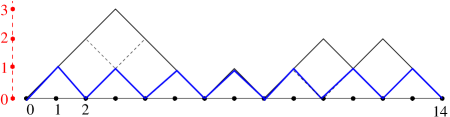
Figure 1: An example of a Dyck path for L = 14. There are four contact points and three clusters. The substrate profile is shown in blue.

A Dyck path is seen as an interface separating a film of tilted tiles deposited on a substrate from a rarefied gas of tiles (see Fig. 2). The stochastic processes in discrete time has two steps:

a) Sequential updating. With a probability $P(i)$ a tile hits the site $i=1,\ldots,L-1$ ($\sum_{i}P(i)=1$). In the RPM, $P(i)$ is chosen uniform: $P(i)=P=1/(L-1)$. In the PARPM, this is not longer the case. For a given configuration $c$ (there are $Z(L)$ of them) with $n_{c}$ peaks. All the peaks are hit with the same probability $R_{p}=p/(L-1)$ ($p$ is a non-negative parameter), all the other $L-1-n_{c}$ sites are hit with the same probability $Q_{c}=q_{c}/(L-1)$. Since

$$n_{c}R_{p}+(L-1-n_{c})Q_{c}=1$$ (2.3)

$q_{c}$ depends on the configuration $c$ and on the parameter $p$, and we have that

$$q_{c}=(L-1-pn_{c})/(L-1-n_{c}),\quad c=1,2,\ldots,Z(L).$$ (2.4)

b) Effects of a hit by a tile. The consequence of the hit on a configuration is the same as in the RPM at the conformal invariant point.

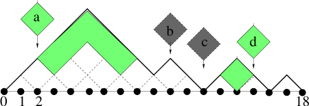
Figure 2: Example of a configuration with 4 peaks of the PARPM for L = 18. Depending on the position where the tilted tiles reach the interface, several distinct processes occur (see the text).

Depending of the slope $s_{i}=(h_{i+1}-h_{i-1})/2$ at the site $i$, the following processes can occur:

1) $s_{i}=0$ and $h_{i}>h_{i-1}$ (tile $b$ in Fig 2). The tile hits a peak and is reflected.

2) $s_{i}=0$ and $h_{i}<h_{i-1}$ (tile $c$ in Fig. 2) . The tile hits a local minimum and is adsorbed ($h_{i}\rightarrow h_{i}+2$).

3) $s_{i}=1$ (tile $a$ in fig. 2). The tile is reflected after triggering the desorption ($h_{j}\rightarrow h_{j}-2$) of a layer of $b-1$ tiles from the segment $\{j=i+1,\ldots,i+b-1\}$ where $h_{j}>h_{i}=h_{i+b}$.

4) $s_{i}=-1$ (tile $d$ in Fig. 2). The tile is reflected after triggering the desorption ($h_{j}\rightarrow h_{j}-2$) of a layer of $b-1$ tiles belonging to the segment $\{j=i-b+1,\ldots,i-1\}$ where $h_{j}>h_{i}=h_{i-b}$.

The continuous time evolution of a system composed by the states $a=1,2,\ldots,Z(L)$ with probabilities $P_{a}(t)$ is given by a master equation that can be interpreted as an imaginary time Schrödinger equation:

$$\frac{d}{dt}P_{a}(t)=-\sum_{b}H_{a,b}P_{b}(t).$$ (2.5)

The Hamiltonian $H$ is an $Z(L)\times Z(L)$ intensity matrix: $H_{a,b}$ ($a\neq b$) is non positive and $\sum_{a}H_{a,b}=0$. $-H_{a,b}$ ($a\neq b$) is the rate for the transition $|b\rangle\rightarrow|a\rangle$. The ground-state wavefunction of the system $|0\rangle$, $H|0\rangle=0$, gives the probabilities in the stationary state:

$$|0\rangle=\sum_{a}P_{a}|a\rangle,\;\;\;\;\;\;P_{a}=\lim_{t\to\infty}P_{a}(t).$$ (2.6)

In order to go from the discrete time description of the stochastic model to the continuous time limit, we take $\Delta t=1/(L-1)$ and

$$H_{ac}=-r_{ac}q_{c}\quad(c\neq a),$$ (2.7)

where $r_{ac}$ are the rates of the RPM and $q_{c}$ is given by Eq. (2.4). The probabilities $R_{p}$ don’t enter in (2.5) since in the RPM when a tile hits a peak, the tile is reflected and the configuration stays unchanged. Notice that through the $q_{c}$’s the matrix elements of the Hamiltonian depend on the size of the system and the numbers of peaks $n_{c}$ of the configurations.

As can be seen from (2.3) and (2.7), for $p<1$ the adsorption and desorption are faster than at $p=1$ and slower for $p>1$. The slowing down is extreme for the substrate where $n_{c}=L/2$. In this case for the value $p=p_{\scriptsize{\mbox{max}}}=2(L-1)/L$ we have $q_{c}=0$ and the substrate becomes an absorbing state.

In a previous paper it was shown that the PARPM is conformal invariant in the domain $0\leq p<p_{\scriptsize{\mbox{max}}}$. The following exact results, which are independent on $p$, are known for this domain.

The average height for large values of the size $L$ of the system is equal to [8, 9]

$$h(L)=\frac{2}{\pi}\int_{\frac{\pi}{L}}^{\frac{\pi}{2}}\frac{\sqrt{3}}{2\pi}\ln(\frac{L}{\pi}\sin x)dx+\beta\approx 0.1056\ln{L}+\beta^{\prime},$$ (2.8)

where $\beta$ and $\beta^{\prime}$ are non universal numbers.

The density of contact points $g(x,L)$ ($x$ is the distance to the origin), in the finite-size scaling limit ($x>>1$, $L>>1$, but $x/L$ fixed) is given by [10]:

$$g(x,L)=C\left(\frac{L}{\pi}\sin(\pi x/L)\right)^{-1/3},$$ (2.9)

where

$$C=-\frac{\sqrt{3}}{6\pi^{5/6}}\Gamma(-1/6)=0.753149...\quad.$$ (2.10)

The average density of minima and maxima (sites where adsorption doesn’t take place) $\tau$(L) has the asymptotic value:

$$\lim_{L\to\infty}\tau(L)=3/4,$$ (2.11)

with non-universal corrections (depending on the value of $p$) of order $1/L$. We will use these results in Sections 3 and 6.

3 Quasistationary states at $p_{\scriptsize{\mbox{max}}}$

When we understood that at $p_{\scriptsize{\mbox{max}}}$ one has an absorbing state, and therefore a phase transition, we got interested to see how conformal invariance is broken. We expected the system to get massive as is the usual case when conformal invariance is broken. It turns out that the new phase is a fascinating object.

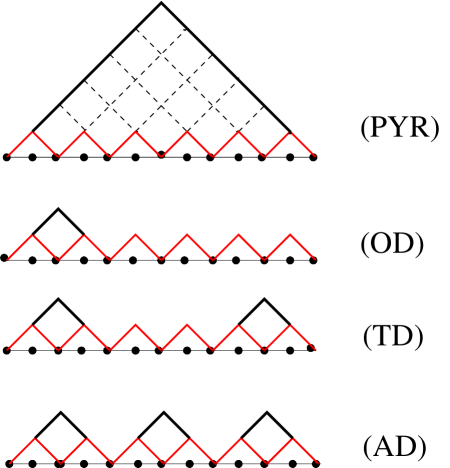
Figure 3: Special initial conditions for $L=12$ (see text).

We have studied several initial conditions specified by the local heights $h_{i}$ (see Fig. 3). One is the ”pyramid” (PYR): the heights are: $0,1,2,3...,L/2,L/2-1,...,1,0$. Another is the ”one dent” (OD): the heights being $0,1,2,1,0,1,0,1,0,...,1,0$. The ”two dent” (TD) one: the heights are: $0,1,2,1,0,1,0,...,0,1,2,1,0$. The ”all dents” (AD) is defined by the local heights: $0,1,2,1,0,1,2,1,0,...,0,1,2,1,0$. We have chosen these four configurations because they are extreme cases. The PYR configuration has only one peak. The OD asymmetric configuration has only one peak less than the substrate which has the maximum number of peaks. The symmetric TD configuration has two peaks less than substrate, the AD configuration is an intermediate one.

We have looked, in Monte Carlo simulations, at the average height from which we have subtracted the average height of the substrate (equal to 1/2), as a function of time taking $L=96$, and starting with the PYR and TD initial conditions. The results of our simulations are shown in Fig. 4. One sees that for each of the two initial conditions one obtains time-independent results which are not zero, as one could expect to find in the absorbing state. This observation suggests the existence of quasistationary states [5, 6].

Figure 4: $p=p_{\scriptsize{\mbox{max}}}$. The average height from which one has subtracted the average height of the substrate ($\frac{1}{2}$), as a function of time for two initial conditions PYR and TD. The lattice size $L=96$. The averages are obtained taking $6\times 10^{5}$ samples.

We have also looked at the average density of clusters $n_{cl}(t)/L$ from which we have subtracted $\frac{1}{2}$ which is the corresponding quantity for the substrate. The results for the two initial conditions PYR and TD are shown in Fig. 5. One obtains similar results as those shown in Figure 4.

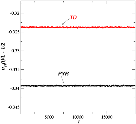
Figure 5: The density of clusters - 1/2 (the density of clusters in the substrate) as a function of time. Same conditions as in Figure 3.

Comparing the average heights and the density of clusters for the two initial conditions, suggest that one has more clusters (therefore lower values of the average height) for the TD initial condition compared to the PYR initial condition. Therefore for $L=96$ the two QSS are different.

Let us make an observation. If we assume that in the QSS one has the same density of clusters as in the stationary distribution observed in the $0\leq p<p_{\scriptsize{\mbox{max}}}$ case [2], for which one has an analytical expression ($n_{cl}/L=\Gamma(1/3)\sqrt{3}/2\pi L^{1/3}$), one obtains the value $-0.339$ for the quantity shown in Fig. 5. This value is closed to the value seen for the PYR initial condition. This observation will play in important role in understanding the QSS.

In order to see how the QSS appeared, we looked for another quantity which was extensively studied in the PARPM [1]. This is the average density of sites where one has a maximum or a minimum in a given configuration $\tau_{\scriptsize{\mbox{max}}}(L,t)$ for $p=p_{\scriptsize{\mbox{max}}}$. In the PARPM and $0\leq p<p_{\scriptsize{\mbox{max}}}$, in the large $L$ limit one has $\tau(L,\infty)=\tau(L)=0.75$ (for the substrate $\tau(L)=1$).

If one starts with the TD configuration and looks at time variation of the quantity $1-\tau_{\scriptsize{\mbox{max}}}(L,t)$ for different system sizes one obtains the results shown in Fig. 6.

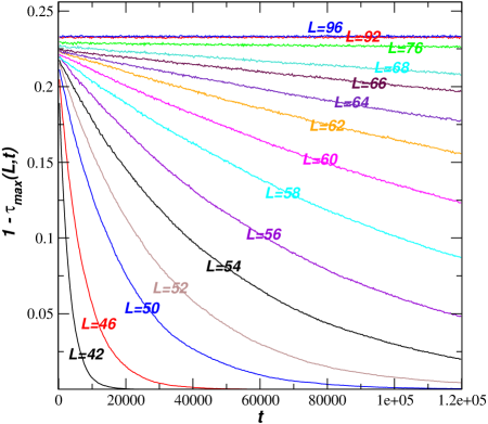
Figure 6: $p=p_{\scriptsize{\mbox{max}}}$. Average density of minima and maxima $\tau_{\scriptsize{\mbox{max}}}(L,t)$ subtracted from 1, as a function of time for different lattices $L$. The initial condition OD was chosen. The averages are obtained by taking $6\times 10^{5}$ samples.

We can see that for small values of $L=46-60$ one has an exponential fall-off with time. Then an almost linear decrease in time for the values $L=62-76$. For $L=92$ and $96$ one sees practically no time variation and a value $\tau_{\scriptsize{\mbox{max}}}(L,t)\sim 0.77$ very close to the value $0.75$ seen in the stationary state in the conformal invariant domain of the model. This makes us suspect the following behavior of $\tau_{\scriptsize{\mbox{max}}}(L,t)$ in the QSS:

$$1-\tau_{\scriptsize{\mbox{max}}}(L,t)=A(L)\exp(-E(L)t),$$ (3.1)

where $E(L)$ decreases exponentially with $L$ and $A(L)$ increases smoothly with $L$ to the value $0.25$ observed for the stationary states in the $0\leq p<p_{\scriptsize{\mbox{max}}}$ domain. In Fig. 7, we show for $L=50$ the data undistinguished from a fit:

$$1-\tau_{\mbox{\scriptsize{max}}}(50,t)=0.217\exp(-0.0000522t).$$ (3.2)

Notice the very small value of $E$ and the fact that $A(50)$ is not far away from the value $0.25$.

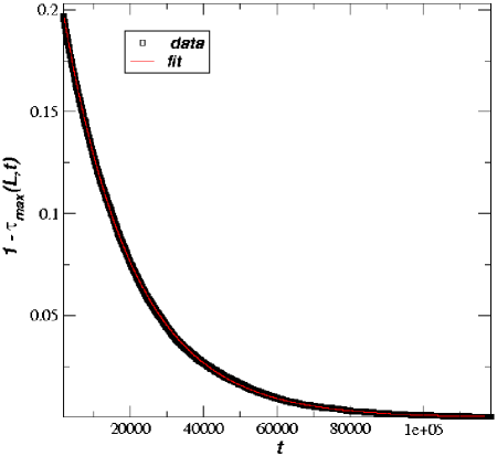
Figure 7: The average density of minima and maxima $\tau(L)$ as a function of time for $L=50$ together with the fit (3.2). The initial configuration is OD and the averages are obtained by taking $6\times 10^{5}$ samples.

We sum up our observations; although for $p=p_{\scriptsize{\mbox{max}}}$ we expected the system to relax in the absorbing state, we observed the existence of states with very long relaxation times. For the lattice sizes presented above, the QSS depend slightly on the initial conditions. Surprisingly, the density of clusters and of maxima and minima in the QSS have values closed to those observed in the stationary states for $0\leq p<p_{\scriptsize{\mbox{max}}}$. Actually for the PYR initial condition the results coincide. In the next three Sections we will explain these observations.

4 The spectrum and wavefunctions of the Hamiltonian. How QSS occur at $p_{\scriptsize{\mbox{max}}}$.

In order to understand the origin of the QSS we have studied the spectrum of the Hamiltonian which gives the time evolution of the system (see Eq. (2.5)). For $0\leq p<p_{\scriptsize{\mbox{max}}}$, where we have conformal invariance, we have checked [1] that in the finite-size scaling limit:

$$\lim_{L\to\infty}E_{i}(L)=\pi v_{s}\Delta_{i}/L,\quad i=0,1,2,\ldots,$$ (4.1)

where $E_{0}=0$, $\Delta_{i}$ are the scaling dimensions, and the sound velocity has the expression:

$$v_{s}(p)=(1-3(p-1)/5)3\sqrt{3}/2.$$ (4.2)

Notice that the velocity decreases when $p>1$ since, as described in Section 2, the transition rates are smaller. The scaling dimensions are given by the partition function [4]:

$$Z(q)=\sum_{i=0}^{\infty}q^{\Delta_{i}}=(1-q)\prod_{n=1}^{\infty}(1-q^{n})^{-1}.$$ (4.3)

We give the first values of $\Delta_{i}$’s together with the corresponding degeneracies ($d_{i}$’s):

$$\Delta=0(1),2(1),3(1),4(2),5(2),6(4),7(4),....$$ (4.4)

We will check if these values will be seen also for $p=p_{\scriptsize{\mbox{max}}}$.

In order to estimate the values of the $\Delta_{i}$’s, we have taken $L=18$ (this is not a small lattice!) and diagonalized numerically the Hamiltonian for various values of $p$. The results are shown in Fig. 8 where the first 11 levels are seen (the ground-state energy $E_{0}$ is equal to zero). The remaining 10 levels should correspond roughly (see (4.4)) to $\Delta=2,3,4,5$ and $6$. We can see that for $p=1$ where the model is integrable, this is indeed the case. The levels cluster in the right places. When $p$ increases, one notices that the properly scaled $E_{1}$ after a smooth behavior up to $p\approx 0.9$, decreases rapidly for $p=p_{\scriptsize{\mbox{max}}}$ (we have used for $v_{s}(p_{\scriptsize{\mbox{max}}})$ the value given by (4.2) for $p=2$). Using Monte Carlo simulations, we have checked [1] that for $p<p_{\scriptsize{\mbox{max}}}$ the small decrease with $p$ of $E_{1}$ is a finite-size effect and therefore what one sees in the figure is a crossover effect. One can also see that for increased values of $p$, $E_{4}$ crosses $E_{3}$ and that $E_{9}$ crosses all the levels $E_{8},\ldots,E_{5}$. Except for the three levels $E_{1},E_{4}$ and $E_{9}$ which decrease dramatically for $p=p_{\scriptsize{\mbox{max}}}$, the other levels have the same finite-size behavior as those in the conformal invariant domain ($p<p_{\scriptsize{\mbox{max}}}$). This suggest that the three levels mentioned above might be related to QSS. We now proceed to a detailed analysis of these observations.

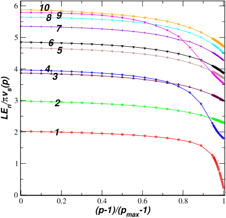
Figure 8: Estimates $\Delta_{n}^{(n)}=LE_{n}/\pi v_{s}(p)$ of the scaling dimensions $\Delta_{n}$ for different values of $p$, and for the lattice size $L=18$. The estimates corresponding to the first 11 energy levels are shown. The values of $v_{s}(p)$ were obtained by (4.2).

Using different lattice sizes we have computed $E_{1}$ as a function of $L$ up to $L=30$. For this calculation we could study larger lattices due to a special property of the Hamiltonian at $p=p_{\scriptsize{\mbox{max}}}$. As we are going to show in section 5, the eigenlevel corresponding to $E_{1}$ is the ground state energy of a reduced matrix defined in a basis where the absorbing state is absent. In this case, by using the power method we were able to calculate $E_{1}$ up to $L=30$. The results can be seen in Fig. 9. Using the two points corresponding to the largest lattice sizes, one obtains:

$$E_{1}(L)=0.912\exp(-0.206L).$$ (4.5)

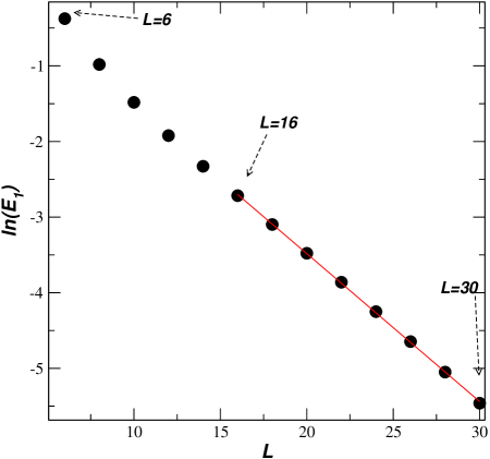
Figure 9: $\ln(E_{1})$ as a function of the lattice size $L$ for $p=p_{\scriptsize{\mbox{max}}}$. The red line is a guide for the eyes, and is obtained from a fit where the lattice sizes $L=16-30$ were used.

To be sure that a power law behavior ($E\approx L^{-m}$) is excluded, we have estimated the derivative $-d/d\ln(L)\{\ln(E_{1}(L))\}$. This quantity should reach a constant for large values of $L$ if $E_{1}(L)$ is power behaved but should diverge linearly in the case of an exponential behavior like (4.5). As seen from Fig. 10, the exponential behavior (4.5) is correct.

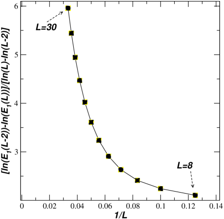
Figure 10: Estimates of $-d/\ln(L)\{\ln(E_{1}(L))\}$ as a function of $1/L$ for different lattice sizes ($p=p_{\scriptsize{\mbox{max}}}$).

A similar analysis of $E_{4}(L)$ but up to $L=18$ only, gives a similar result:

$$E_{4}(L)=2.41\exp(-0.10L).$$ (4.6)

We have not looked at $E_{9}(L)$ but we expect again an exponential fall-off. We conclude that three energy levels have an exponential fall-off and that they can be related to QSS. This is going to be shown to be the case in Section 5. We proceed by looking at the remaining levels.

The data suggest that at $p=p_{\scriptsize{\mbox{max}}}$, the energy levels that do not go exponentially to zero have the same finite-size scaling behavior as those in the conformal invariant domain. This would imply that instead of (4.4) we would have

$$\Delta=0(1),3(1),4(1),5(2),6(3),\ldots\quad.$$ (4.7)

If confirmed, this would lead us to a strange picture since the scaling dimension $\Delta=2$ does not appear. This dimension corresponds to the energy-momentum, and therefore conformal invariance couldn’t apply and we could not explain the finite-size behavior of the remaining levels. What can go wrong in our picture? One possibility is that the finite-size scaling of the levels doesn’t satisfy (4.1).

We have computed $E_{2}(L)$ up to $L=18$. A fit to the data gives $\Delta_{3}=3.05$ in agreement with what should be expected. Similarly examining $E_{4}(L)$ one finds $\Delta_{4}=3.95$ also as expected. These estimates were found assuming that $v_{s}(p_{\scriptsize{\mbox{max}}})$ is given by Eq. (4.2). Can we get $\Delta=2$ changing the sound velocity such that $E_{3}(L)$ gives $\Delta=2$, $E_{5}(L)$ gives $\Delta=3$, $E_{6}(L)$ gives $\Delta=4,\ldots$? We have computed the ratios $E_{5}(L)/E_{3}(L)$ and $E_{6}(L)/E_{3}(L)$ as a function of $L$. One should obtain 4/3 respectively 5/3 if one had (4.3) and 3/2 respectively 2 if the energy momentum tensor would be present. In Figs. 11 and 12 we show these ratios as functions of $1/L$. Cubic fits give the values 1.32 respectively 1.64. We conclude that (4.7) is most probably correct. We have also checked that there are no energy crossings for the levels which cluster around $\Delta=7$.

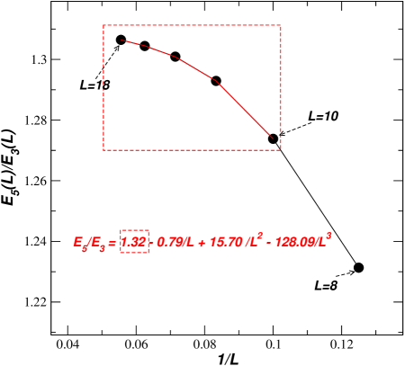
Figure 11: Ratio among the two lowest eigenenergies, at $p=p_{\scriptsize{\mbox{max}}}$,that does not vanish exponentially. The data are plotted as a function of $1/L$, for lattice sizes $L=8-18$. A cubic fit was done by using the five largest lattice sizes.

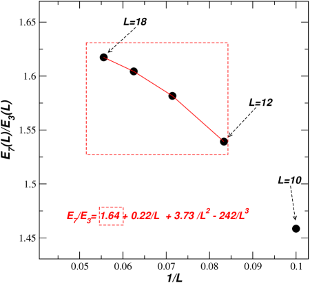
Figure 12: Ratio among the third and second lowest eigenenergies, at $p=p_{\scriptsize{\mbox{max}}}$,that does not vanish exponentially. The data are plotted as a function of $1/L$, for lattice sizes $L=10-18$. A cubic fit was done by using the four largest lattice sizes.

The analysis of the energy levels (compare (4.4) with (4.7)) suggests that at $p=p_{\scriptsize{\mbox{max}}}$ the partition function (4.3) changes in the following way: the degeneracy at each even value of $\Delta$ decreases with one unit. Each energy level which left the Virasoro representation at non-zero even values of $\Delta$ moves to $\Delta$ = 0 which becomes infinitely degenerate. This opens a problem in the representation theory of the algebra which might be solvable since the central charge is c = 0. In Section 6 we are going to learn more about this puzzle.

5 From eigenfunctions of the Hamiltonian to QSS

We have seen in the last section that some eigenvalues of the Hamiltonian vanish exponentially. Here we will show what is their connection to QSS. In order to do so, we first prove a special property of Hamiltonians in the presence of an absorbing state.

We denote the vector space corresponding to $n+1$ configurations by $|0\rangle$, $|i\rangle$ ($i=1,2,...,n$), in which we have chosen $|0\rangle$ to be the absorbing state. The Hamiltonian has the following properties:

$$H_{i,0}=0,\quad H_{0,0}=0,\quad H_{i,j}\leq 0,$$ (5.1)

$$H_{0,j}+\sum_{i}H_{i,j}=0\quad(j=1,2,...n).$$ (5.2)

Assume that $E_{k}$ ($k=1,...,n$) is a non-vanishing eigenvalue of $H$ with an eigenvector ($y_{0}^{(k)},y_{1}^{(k)},...,y_{n}^{(k)}$). We can show that the sum of the components of any eigenvector is equal to zero:

$$y_{0}^{(k)}+\sum_{i}y_{i}^{(k)}=0\quad(k=1,2,..,n).$$ (5.3)

Using (5.1) and (5.2) we have:

$$E_{k}y_{0}^{(k)}=\sum_{i}H_{0,i}y_{i}^{(k)}=-\sum_{j,i}H_{j,i}y_{i}^{(k)}=-E_{k}\sum_{j}y_{j}^{(k)},$$ (5.4)

from which the identity (5.3) follows.

We consider now the reduced matrix $H^{\prime}_{i,j}=H_{i,j}$ ($i,j=1,2,...,n$) (the configuration $|0\rangle$ is taken out). Let $E_{1}$ be the lowest non-vanishing eigenvalue, from (5.1) and using the Perron Frobenius theorem, we get:

$$y_{i}^{(1)}\geq 0,$$ (5.5)

and using (5.3), $y_{0}^{(1)}<0$. From the same theorem we also learn that $E_{1}$ is the unique eigenvalue for which (5.5) occurs. For the other eigenvalues, at least one component of the wavefunction is negative, i. e. Eq. (5.5) is not valid for $y_{i}^{(k)}$ ($k>1$).

The solutions of the differential equations (2.5) are

$$P_{0}(t)=1+\sum_{k}A_{k}y_{0}^{(k)}\exp(-E_{k}t),$$

$$P_{i}(t)=\sum_{k}A_{k}y_{i}^{(k)}\exp(-E_{k}t).$$ (5.6)

The $n$ constants $A_{k}$ are determined from the initial conditions.

At large values of $L$ and $t$, the exponentially falling energies give the major contributions to $P_{0}(t)$ and $P_{i}(t)$. Among them, $E_{1}$ plays a special role. Note only is $E_{1}$ the smallest energy, but the components of its eigenfunction are positive (5.5). This implies that for a large range of $L$ and $t$ (both of them large), one can keep only the term with $k=1$ in the sums appearing in (5.6). The situation is different at very large values of $L$ when all the exponentially falling energies are practically equal to zero and more terms can appear in (5.6). Independent of the initial conditions, the term with $k=1$ has to be present in the sums (5.6) in order to assure the positivity of the probabilities $P_{0}(t)$ and $P_{i}(t)$ since for the other eigenfunctions (5.5) is not valid. For example, the eigenfunctions corresponding to the levels $E_{4}(L)$ and $E_{9}(L)$ of Fig. 8 have components with both signs in the sum giving $P_{i}(t)$.

We are now in the position to show how exponentially falling energies like $E_{1}(L)$ (see (4.5)) can be the origin of QSS. For our discussion we will assume that the term with $k=1$ alone is present in (5.6). It turns out that this assumption will help to explain all the results obtained for the Monte Carlo simulations. The probability vector $|P(t,L)\rangle$ becomes:

$$|P(t,L)\rangle=[1-a(L)\exp(-E_{1}(L)t)]|0\rangle+a(L)\sum_{i}p_{i}(L)|i\rangle\exp(-E_{1}(L)t),$$ (5.7)

where we have used (5.3) and (5.5)

$$a(L)=A_{1}\sum_{i}y_{i}^{(1)}(L);\quad p_{i}(L)=y_{i}^{(1)}(L)/\sum_{i}y_{i}^{(1)}(L).$$ (5.8)

Note that $p_{i}(L)$ gives the probability to find the system in configuration $|i\rangle$ if the system is in the stationary state of the reduced Hamiltonian $H^{\prime}$, that acts in the vector space where the substrate is absent. Thus, Equation (5.7) explains the occurrence of QSS. If $L$ is large enough, $E_{1}(L)$ is negligible, one finds:

$$|P(L)\rangle=(1-a(L))|0\rangle+a(L)|P_{\mbox{\scriptsize ns}}(L)\rangle.$$ (5.9)

Here $a(L)$ depends on the initial conditions and it is not equal to zero. $|P_{\mbox{\scriptsize ns}}(L)\rangle$ is a probability distribution function of configurations in which the substrate is not present. Equation (5.9) describes therefore the QSS. Using Monte Carlo simulations we have measured the probability to find the system in the substrate. For the OD initial condition (see Section 3 for the definition), one finds:

$$1-a(L)\sim 4.5/L.$$ (5.10)

For the PYR initial condition one finds $1-a(L)=10^{-5}$ for $L=96$ (we didn’t compute $a(L)$ for the TD and AD initial conditions). This implies that for large values of $L$ one has

$$|P(L)\rangle=|P_{\mbox{\scriptsize ns}}(L)\rangle,$$ (5.11)

and the substrate does not occur in the QSS. We postpone the discussion of the results shown in Fig. 6 up to the next Section.

6 The quasistationary states

In this section we are going to identify the quasistationary states observed in the Monte Carlo simulations (see Figs. 4-7) and find a puzzle. The basis of our identification are Eqs. (5.7), (5.9) and (5.11).

We have taken large lattices and started our simulations with the PYR initial condition. We first looked at the average height $h(L)$. The results are shown in Fig. 13. The data can be fitted by a straight line. Taking only the two largest lattice sizes we obtain:

$$h(L)=0.1068\ln(L)+0.042.$$ (6.1)

In astonishing agreement with the expression (2.8) derived [8, 9] assuming conformal invariance and used to describe the data for $0\leq p<p_{\scriptsize{\mbox{max}}}$. Since for the large lattices we have considered, we can use (5.11) and this would imply that $|P_{\mbox{\scriptsize ns}}(L)\rangle$ is given by the same function as the one seen away from $p_{\scriptsize{\mbox{max}}}$.

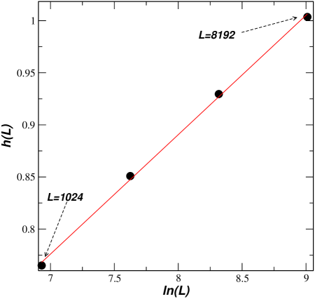
Figure 13: The average height $h(L)$ as a function of $\ln(L)$ in the QSS. $L=1024,2048,4096$ and $8192$. We have used PYR as an initial distribution.

If confirmed, this result would be surprising because as we have discussed in Section 4, as compared to the conformal invariant domain, at $p=p_{\scriptsize{\mbox{max}}}$ the finite-size spectrum of the Hamiltonian is a ”mutilated” one. It lacks not only the energy momentum tensor but other levels too. On the other hand that space-like correlation functions look to be unaffected.

In Fig. 14 we show for the AD initial condition, the density of contact points $g(x,L)$ for various lattice sizes divided by the finite-size scaling distribution (2.9) in the QSS. The coincidence of the $p_{\scriptsize{\mbox{max}}}$ data and the expectation coming from conformal invariance in the QSS is astonishing (for the large lattices considered here $a(L)$ is practically equal to 1).

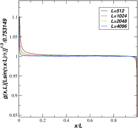
Figure 14: The density of contact points $g(x,L)$ as a function of $x/L$ at $p_{\scriptsize{\mbox{max}}}$, divided by (2.9). $L=1024,2048,4096$ and $8192$. Initial condition AD. The average are obtained from 3500 samples running $10^{6}$ mcsteps.

From now on, we will assume that for large lattices the QSS the correlators are those of the conformal invariant model (RPM) and will try to explain the results described in Section 3.

We use Eq. (5.9) and the observation that for the initial condition PYR $a(L)=1$, taking $a(96)=0.975$ for the TD initial condition we obtain the results for TD presented in both Figs. 4 and 5 (we don’t have at hand an independent measurement of $a(L)$ for the TD initial condition).

We proceed by looking for a description of the data presented in Fig. 6, where the time dependence of the quantity $1-\tau_{\scriptsize{\mbox{max}}}(L,t)$, taking OD initial condition, is shown. $\tau_{\scriptsize{\mbox{max}}}(L,t)$ is the average density of minima and maxima which is equal to 1 for the substrate. We use Eqs. (5.7) and (5.10) to get:

$$1-\tau_{\scriptsize{\mbox{max}}}(L,t)=[-4.5/L+1-(1-4.5/L)\tau(L)]\exp(-E_{1}(L)t).$$ (6.2)

The function $\tau(L)$ is known analytically only for $p=1$ [2]. It is equal to $3/4$ in the large $L$ limit and has non-universal corrections of order $1/L$ which are unknown for $p=p_{\scriptsize{\mbox{max}}}$. In principle these corrections can be determined by looking at the QSS obtained using PYR initial conditions. We can however use the result obtained in [1] for $p=1.99$ where we found $\tau(L)\approx 0.75-0.3/L$ and use it in (6.2) to get a fair description of the data. We obtain

$$1-\tau_{\scriptsize{\mbox{max}}}(L,t)\approx(0.25-0.8/L)\exp(-E_{1}(L)t).$$ (6.3)

The value of $E_{1}(L)$ can be estimated from (4.5). In Fig. 15 we use this function, together with the predicted values of $E_{1}(L)$ given in (4.5), to compute the time dependence of $1-\tau_{\scriptsize{\mbox{max}}}(L,t)$ for the same lattice sizes used in Fig. 6. We can see that the overall behavior of Fig. 15 and Fig. 6, generated by the Monte carlo simulations, are the same.

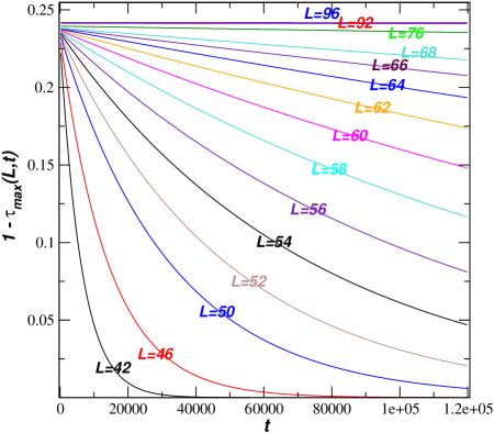
Figure 15: The average density of minima and maxima $\tau_{\scriptsize{\mbox{max}}}(L,t)(L,t)$ subtracted from 1, as a function of time for the same lattice sizes $L$, as in Fig 6. The initial condition is OD. The data were generated from the prediction (6.3), using $E_{1}$ given by (4.5)

7 Conclusions

The parameter $p$ which enters in the definition of peak adjusted raise and peel stochastic model determines a domain $0\leq p<p_{\scriptsize{\mbox{max}}}$ in which one has conformal invariance. In the finite-size scaling regime all the properties are independent on $p$ which appears only in the sound velocity $v_{s}(p)$ which fixes the time scale. If $p>1$, global properties of the configurations (the number of peaks) and the size of the system $L$, enter in the rates. The larger is the number of peaks of a configuration, the smaller are the rates to escape the configuration. As a result, at $p=p_{\scriptsize{\mbox{max}}}=2(L-1)/L$ the configuration with the largest number of peaks which is the substrate, becomes an absorbtive state for any size of the system. Since there are no fluctuations in the ground-state of the system, we expect conformal invariance to be lost and get into a massive phase. This is not the case and a fascinating phenomenon takes place.

The new features of the model at $p=p_{\scriptsize{\mbox{max}}}$ are encoded in Figures 4 and 6. If the evolution of the system starts with a given initial configuration, instead of moving fast to the absorbing state, the system gets stuck in another configuration and the relaxation time grows exponentially with the size of the system. This is a quasistationary state. In Figure 8 we look at the spectrum of the Hamiltonian and follow the change of the scaled energies with increasing values of the parameter $p$. From the eleven energy levels shown in the figure, eight of them are those of the conformal invariant region ($0\leq p<p_{\scriptsize{\mbox{max}}}$). Three of them go exponentially to zero for large values of $L$.

In this paper we have tried to clarify this phenomenon. Based, unfortunately, on numerics, the following picture emerges. The wavefunction corresponding to the first excited state whose energy vanishes exponentially, gives the probability distribution function of the QSS. This is due to a peculiar property of the first exited state of any stochastic Hamiltonian in the presence of an absorbing state. For finite values of $L$, the QSS depends on the initial conditions but in the thermodynamical limit, it becomes independent of them. Unexpectedly, the finite-size scaling properties of the QSS are identical to the one observed for the ground-state in the conformal invariant domain.

This picture describes a strange way to break conformal invariance. Part of the spectrum stays unchanged (not the scaling dimension of the energy-momentum tensor!) and another part sinks in the vacuum which becomes probably infinite degenerate. We have not a clue how to explain this observation. At the same time, the space-like correlations seen in the QSS are those of the conformal domain. This is obviously an unexplained paradox. The study of space-time correlation functions should shade light in this problem. We plan to do it in the future.

We have studied only four initial conditions and found essentially only one QSS. This QSS could be related to the eigenfunction corresponding to the first exited state. It is most probable that we have missed other QSS which should be related to some linear combination of eigenfunctions corresponding to the remaining exponentially decaying energies.

The search for QSS should continue in some extensions of the PARPM. One can look at the fate of defects like those studied in [11] when the rates are adjusted to the number of peaks. Another interesting avenue is to study the effect of changing the rates depending on the number of peaks in the extension [2, 3] of the raise and peel model in which the rates of adsorption and desorption are not equal.

8 Acknowledgments

We would like to thank S. Ruffo, H. Hinrichsen, A. Bovier and J. A. Hoyos for reading the manuscript and discussions. This work was supported in part by FAPESP and CNPq (Brazilian Agencies). Part of this work was done while V.R. was visiting the Weizmann Institute. V. R. would like to thank D. Mukamel for his hospitality and the support of the Israel Science Foundation (ISF) and the Minerva Foundation with funding from the Federal German Ministry for Education and Research.

References

- [1] Alcaraz F C and Rittenberg V, 2007 J. Stat. Mech. P12032
- [2] de Gier J, Nienhuis B, Pearce P and Rittenberg V, 2003 J. Stat. Phys. 114 1
- [3] Alcaraz F C and Rittenberg V, 2007 J. Stat. Mech. P07009
- [4] Read N and Saleur H, 2001 Nucl. Phys. B 613 409
- [5] Campa A, Dauxois T and Ruffo S, 2009 Phys. Rep. 480 57
- [6] Mukamel D, 2008 in Lecture Notes at Summer School in Les Houches (France), 4-29
- [7] Evans M R, Kafri Y, Koduvely H M and Mukamel D, 1998 Phys. Rev. E 58 2764
- [8] Jacobsen J L, and Saleur H, 2008 Phys. Rev. Lett. 100 087205
- [9] Alcaraz F C and Rittenberg V, 2010 J. Stat. Mech. P03024
- [10] Alcaraz F C, Pyatov P and Rittenberg V, 2007 J. Stat. Mech. P07009
- [11] Alcaraz F C and Rittenberg V, 2007 Phys. Rev. E 75 051110