Topological Casimir effect in compactified cosmic string spacetime

Abstract

We investigate the Wightman function, the vacuum expectation values of the field squared and the energy-momentum tensor for a massive scalar field with general curvature coupling in the generalized cosmic string geometry with a compact dimension along its axis. The boundary condition along the compactified dimension is taken in general form with an arbitrary phase. The vacuum expectation values are decomposed into two parts. The first one corresponds to the uncompactified cosmic string geometry and the second one is the correction induced by the compactification. The asymptotic behavior of the vacuum expectation values of the field squared, energy density and stresses are investigated near the string and at large distances. We show that the nontrivial topology due to the cosmic string enhances the vacuum polarization effects induced by the compactness of spatial dimension for both the field squared and the vacuum energy density. A simple formula is given for the part of the integrated topological Casimir energy induced by the planar angle deficit. The results are generalized for a charged scalar field in the presence of a constant gauge field. In this case, the vacuum expectation values are periodic functions of the component of the vector potential along the compact dimension.

PACS numbers: 98.80.Cq, 11.10.Gh, 11.27.+d

1 Introduction

Within the framework of grand unified theories, as a result of vacuum symmetry breaking phase transitions, different types of topological defects could be produced in the early universe [1, 2]. In particular, cosmic strings have attracted considerable attention. Although the recent observational data on the cosmic microwave background have ruled out cosmic strings as the primary source for large scale structure formation, they are still candidates for a variety of interesting physical phenomena such as the generation of gravitational waves [3], high energy cosmic rays [4], and gamma ray bursts [5]. Recently the cosmic strings attracted a renewed interest partly because a variant of their formation mechanism is proposed in the framework of brane inflation [6].

In the simplest theoretical model describing the infinite straight cosmic string the spacetime is locally flat except on the string where it has a delta shaped curvature tensor. The corresponding nontrivial topology raises a number of interesting physical effects. One of these concerns the effect of a string on the properties of quantum vacuum. Explicit calculations for vacuum polarization effects in the vicinity of a string have been done for various fields [7]-[22]. Vacuum polarization effects by the cosmic string carrying a magnetic flux are considered in Ref. [23]. Another type of topological quantum effects appears in models with compact spatial dimensions. The presence of compact dimensions is a key feature of most high energy theories of fundamental physics, including supergravity and superstring theories. An interesting application of the field theoretical models with compact dimensions recently appeared in nanophysics. The long-wavelength description of the electronic states in graphene can be formulated in terms of the Dirac-like theory in three-dimensional spacetime with the Fermi velocity playing the role of speed of light (see, e.g., [24]). Single-walled carbon nanotubes are generated by rolling up a graphene sheet to form a cylinder and the background spacetime for the corresponding Dirac-like theory has topology $R^{2}\times S^{1}$. The compactification of spatial dimensions serves to alter vacuum fluctuations of a quantum field and leads to the Casimir-type contributions in the vacuum expectation values of physical observables (see Refs. [25, 26] for the topological Casimir effect and its role in cosmology). In the Kaluza-Klein-type models, the topological Casimir effect induced by the compactification has been used as a stabilization mechanism for the size of extra dimensions. The Casimir energy can also serve as a model for dark energy needed for the explanation of the present accelerated expansion of the universe. The influence of extra compact dimensions on the Casimir effect in the classical configuration of two parallel plates has been recently discussed for the case of a scalar field [27], for the electromagnetic field with perfectly conducting boundary conditions [28], and for a fermionic field with bag boundary conditions [29].

In this paper we shall study the configuration with both types of sources for the vacuum polarization, namely, a generalized cosmic string spacetime with a compact spatial dimension along its axis (for combined effects of topology and boundaries on the quantum vacuum in the geometry of a cosmic string see [30, 31, 32]). For a massive scalar field with an arbitrary curvature coupling parameter, we evaluate the Wightman function, the vacuum expectation values of the field squared and the energy-momentum tensor. These expectation values are among the most important quantities characterizing the vacuum state. Though the corresponding operators are local, due to the global nature of the vacuum, the vacuum expectation values carry an important information about the the global properties of the bulk. In addition, the vacuum expectation value of the energy-momentum tensor acts as the source of gravity in the semiclassical Einstein equations. It therefore plays an important role in modelling a self-consistent dynamics involving the gravitational field. The problem under consideration is also of separate interest as an example with two different kind of topological quantum effects, where all calculations can be performed in a closed form.

We have organized the paper as follows. The next section is devoted to the evaluation of the Wightman function for a massive scalar field in a generalized cosmic string spacetime with a compact dimension. Quasiperiodic boundary condition with an arbitrary phase is assumed along the compact dimension . By using the formula for the Wightman function, in section 3 we evaluate the vacuum expectation value of the field squared. This expectation value is decomposed into two parts: the first one corresponding to the geometry of a cosmic string without compactification and the second one being induced by the compactification. The vacuum expectation value of the energy-momentum tensor is discussed in section 4. Section 5 is devoted to the investigation of the part in topological vacuum energy induced by the planar angle deficit. Finally, the results are summarized and discussed in section 6.

2 Wightman function

We consider a $(D+1)$-dimensional generalized cosmic string spacetime. Considering the generalized cylindrical coordinates $(x^{1},x^{2},\ldots,x^{D})=(r,\phi,z,x^{4},\ldots,x^{D})$ with the string on the $(D-2)$ -dimensional hypersurface $r=0$, the corresponding geometry is described by the line element

$$ds^{2}=g_{ik}dx^{i}dx^{k}=dt^{2}-dr^{2}-r^{2}d\phi^{2}-dz^{2}-\sum_{l=4}^{D}(dx^{l})^{2}.$$ (1)

The coordinates take values in the ranges $r\geqslant 0$, $0\leqslant\phi\leqslant\phi_{0}$, $-\infty<x^{l}<+\infty$ for $l=4,\ldots,D$, and the spatial points $(r,\phi,z,x^{4},\ldots,x^{D})$ and $(r,\phi+\phi_{0},x^{4},\ldots,x^{D})$ are to be identified. Additionally we shall assume that the direction along the $z$-axis is compactified to a circle with the length $L$: $0\leqslant z\leqslant L$ (about the generalization of the model in the case of an arbitrary number of compact dimensions along the axis of the string see below). In the standard $D=3$ cosmic string case with $-\infty<z<+\infty$, the planar angle deficit is related to the mass per unit length of the string $\mu$ by $2\pi-\phi_{0}=8\pi G\mu$, where $G$ is the Newton gravitational constant.

It is interesting to note that the effective metric produced in superfluid ${}^{3}\mathrm{He-A}$ by a radial disgyration is described by the $D=3$ line element (1) with the negative planar angle deficit [33]. In this condensed matter system the role of the Planck energy scale is played by the gap amplitude. The graphitic cones are another class of condensed matter systems, described in the long wavelength approximation by the metric (1) with $D=2$. Graphitic cones are obtained from the graphene sheet if one or more sectors are excised. The opening angle of the cone is related to the number of sectors removed, $N_{c}$, by the formula $2\pi(1-N_{c}/6)$, with $N_{c}=1,2,\ldots,5$. All these angles have been observed in experiments [34]. Induced fermionic current and fermionic condensate in a $(2+1)$-dimensional conical spacetime in the presence of a circular boundary and a magnetic flux have been recently investigated in Ref. [35].

In this paper we are interested in the calculation of one-loop quantum vacuum effects for a scalar quantum field $\varphi(x)$, induced by the non-trivial topology of the $z$-direction in the geometry (1). For a massive field with curvature coupling parameter $\xi$ the field equation has the form

$$\left(\nabla^{i}\nabla_{i}+m^{2}+\xi R\right)\varphi(x)=0,$$ (2)

where $\nabla_{i}$ is the covariant derivative operator and $R$ is the scalar curvature for the background spacetime. In the geometry under consideration $R=0$ for $r\neq 0$. The values of the curvature coupling parameter $\xi=0$ and $\xi=\xi_{D}\equiv(D-1)/4D$ correspond to the most important special cases of minimally and conformally coupled scalars, respectively. We assume that along the compact dimension the field obeys quasiperiodicity condition

$$\varphi(t,r,\phi,z+L,x^{4},\ldots,x^{D})=e^{2\pi i\beta}\varphi(t,r,\phi,z,x^{4},\ldots,x^{D}),$$ (3)

with a constant phase $\beta$, $0\leqslant\beta\leqslant 1$. The special cases $\beta=0$ and $\beta=1/2$ correspond to the untwisted and twisted fields, respectively, along the $z$-direction. We could also consider quasiperiodicity condition with respect to $\phi\rightarrow\phi+\phi_{0}$. This would correspond to a cosmic string which carries an internal magnetic flux. Though the corresponding generalization is straightforward, for simplicity we shall consider a string without a magnetic flux.

In quantum field theory, the imposition of the condition (3) changes the spectrum of the vacuum fluctuations compared to the case with uncompactified dimension. As a consequence, the vacuum expectation values (VEVs) of physical observables are changed. The properties of the vacuum state are described by the corresponding positive frequency Wightman function, $W(x,x^{\prime})=\langle 0|\varphi(x)\varphi(x^{\prime})|0\rangle$, where $|0\rangle$ stands for the vacuum state. In particular, having this function we can evaluate the VEVs of the field squared and the energy-momentum tensor. In addition, the response of particle detectors in an arbitrary state of motion is determined by this function (see, for instance, [36, 37]). For the evaluation of the Wightman function we use the mode sum formula

$$W(x,x^{\prime})=\sum_{\mathbf{\alpha}}\varphi_{\mathbf{\alpha}}(x)\varphi_{\mathbf{\alpha}}^{\ast}(x^{\prime}),$$ (4)

where $\{\varphi_{\mathbf{\alpha}}(x),\varphi_{\mathbf{\alpha}}^{\ast}(x)\}$ is a complete set of normalized mode functions satisfying the periodicity condition (3) and $\alpha$ is a collective notation for the quantum numbers specifying the solution.

In the problem under consideration, the mode functions are specified by the set of quantum numbers $\alpha=(n,\gamma,k_{z},\mathbf{k})$, with the values in the ranges $n=0,\pm 1,\pm 2,\ldots$, $\mathbf{k}=(k_{4},\ldots,k_{D})$, $-\infty<k_{l}<\infty$. The mode functions have the form

$$\varphi_{\alpha}(x)=\frac{q\gamma J_{q\left|n\right|}(\gamma r)}{2(2\pi)^{D-2}\omega L}\exp\left(iqn\phi+ik_{z}z+i\mathbf{kr}_{\parallel}-i\omega t\right),$$ (5)

where $J_{\nu}(z)$ is the Bessel function, $\mathbf{r}_{\parallel}=(x^{4},\ldots,x^{D})$ and

$$\omega=\sqrt{\gamma^{2}+k_{z}^{2}+k^{2}+m^{2}},\quad q=2\pi/\phi_{0}.$$ (6)

From the periodicity condition (3), for the eigenvalues of the quantum number $k_{z}$ one finds

$$k_{z}=2\pi(l+\beta)/L,\;l=0,\pm 1,\pm 2,\ldots.$$ (7)

Substituting the mode functions (5) into the sum (4), for the positive frequency Wightman function one finds

$$W(x,x^{\prime}) = \frac{q}{(2\pi)^{D-2}L}\sideset{}{{}^{\prime}}{\sum}_{n=0}^{\infty}\cos(qn\Delta\phi)\int d\mathbf{k}\,e^{i\mathbf{k}\Delta\mathbf{r}_{\parallel}}$$ (8)

$$\times\int_{0}^{\infty}d\gamma\,\gamma J_{qn}(\gamma r)J_{qn}(\gamma r^{\prime})\sum_{l=-\infty}^{\infty}\frac{e^{-i\omega\Delta t+ik_{z}\Delta z}}{\omega},$$

where $\Delta\phi=\phi-\phi^{\prime}$, $\Delta\mathbf{r}_{\parallel}=\mathbf{r}_{\parallel}-\mathbf{r}_{\parallel}^{\prime}$, $\Delta t=t-t^{\prime}$, $\Delta z=z-z^{\prime}$, and the prime on the sum over $n$ means that the summand with $n=0$ should be taken with the weight 1/2. For the further evaluation, we apply to the series over $l$ the Abel-Plana summation formula in the form [38] (for generalizations of the Abel-Plana formula and their applications in quantum field theory see [25, 39, 40])

$$\sum_{l=-\infty}^{\infty}g(l+\beta)f(|l+\beta|)=\int_{0}^{\infty}du\,\left[g(u)+g(-u)\right]f(u)$$

$$\qquad+i\int_{0}^{\infty}du\left[f(iu)-f(-iu)\right]\sum_{\lambda=\pm 1}\frac{g(i\lambda u)}{e^{2\pi(u+i\lambda\beta)}-1}.$$ (9)

In the special case of $g(y)=1$ and $\beta=0$ this formula is reduced to the standard Abel-Plana formula. Taking in Eq. (9)

$$g(y)=e^{2\pi iy\Delta z/L},\;f(y)=\frac{e^{-i\Delta t\sqrt{(2\pi y/L)^{2}+\gamma^{2}+k^{2}+m^{2}}}}{\sqrt{(2\pi y/L)^{2}+\gamma^{2}+k^{2}+m^{2}}},$$ (10)

we present the Wightman function in the decomposed form

$$W(x,x^{\prime})=W_{\text{s}}(x,x^{\prime})+\frac{2q}{(2\pi)^{D-1}}\sideset{}{{}^{\prime}}{\sum}_{n=0}^{\infty}\cos(qn\Delta\phi)\int d\mathbf{k}\,e^{i\mathbf{k}\Delta\mathbf{r}_{\parallel}}\int_{0}^{\infty}d\gamma\,\gamma J_{qn}(\gamma r)$$

$$\qquad\times J_{qn}(\gamma r^{\prime})\int_{\sqrt{\gamma^{2}+k^{2}+m^{2}}}^{\infty}dy\frac{\cosh(\Delta t\sqrt{y^{2}-\gamma^{2}-k^{2}-m^{2}})}{\sqrt{y^{2}-\gamma^{2}-k^{2}-m^{2}}}\sum_{\lambda=\pm 1}\frac{e^{-\lambda y\Delta z}}{e^{Ly+2\pi i\lambda\beta}-1},$$ (11)

where $W_{\text{s}}(x,x^{\prime})$ is the Wightman function in the geometry of a cosmic string without compactification. The latter corresponds to the first term on the right hand side of (9). The integration over the angular part of $\mathbf{k}$ is done with the help of the formula

$$\int d\mathbf{k}\,e^{i\mathbf{k}\Delta\mathbf{r}_{\parallel}}F(k)=\frac{(2\pi)^{(D-3)/2}}{|\Delta\mathbf{r}_{\parallel}|^{(D-5)/2}}\int_{0}^{\infty}dk\,k^{(D-3)/2}J_{(D-5)/2}(k|\Delta\mathbf{r}_{\parallel}|)F(k),$$ (12)

for a given function $F(k)$. By using the expansion $[e^{Ly+2\pi i\lambda\beta}-1]^{-1}=\sum_{l=1}^{\infty}e^{-lLy-2\pi il\lambda\beta}$, the further integrations over $k$ and $y$ are done by making use of formulas from [41]. Similar transformations are done for the part $W_{\text{s}}(x,x^{\prime})$. As a result we find the following expression

$$W(x,x^{\prime}) = \frac{2q}{(2\pi)^{(D+1)/2}}\sideset{}{{}^{\prime}}{\sum}_{n=0}^{\infty}\cos(qn\Delta\phi)\int_{0}^{\infty}d\gamma\,\gamma J_{qn}(\gamma r)J_{qn}(\gamma r^{\prime})$$ (13)

$$\times\sum_{l=-\infty}^{\infty}e^{-2\pi li\beta}\left(\gamma^{2}+m^{2}\right)^{(D-3)/2}f_{(D-3)/2}(w_{l}\sqrt{\gamma^{2}+m^{2}}),$$

where

$$w_{l}^{2}=\left(\Delta z+lL\right)^{2}+|\Delta\mathbf{r}_{\parallel}|^{2}-(\Delta t)^{2},$$ (14)

and we use the notation

$$f_{\nu}(x)=K_{\nu}(x)/x^{\nu}.$$ (15)

The term $l=0$ in (13) corresponds to the function $W_{\text{s}}(x,x^{\prime})$.

For the further transformation of the expression (13) we employ the integral representation of the modified Bessel function [42],

$$K_{\nu}(y)=\frac{1}{2^{\nu+1}y^{\nu}}\int_{0}^{\infty}d\tau\frac{e^{-\tau y^{2}-1/(4\tau)}}{\tau^{\nu+1}}.$$ (16)

Substituting this representation in (13), the integration over $\gamma$ is done explicitly. Introducing an integration variable $u=1/(2\tau)$ and by changing $l\rightarrow-l$, one finds

$$W(x,x^{\prime})=\frac{q}{(2\pi)^{(D+1)/2}}\sum_{l=-\infty}^{\infty}e^{2\pi li\beta}\int_{0}^{\infty}du\,u^{(D-3)/2}e^{-u_{l}^{2}u/2-m^{2}/(2u)}\sideset{}{{}^{\prime}}{\sum}_{n=0}^{\infty}\cos(qn\Delta\phi)I_{qn}(urr^{\prime}),$$ (17)

where

$$u_{l}^{2}=r^{2}+r^{\prime 2}+\left(\Delta z-lL\right)^{2}+|\Delta\mathbf{r}_{\parallel}|^{2}-(\Delta t)^{2}.$$ (18)

The expression for the Wightman function may be further simplified by using the formula

$$\sideset{}{{}^{\prime}}{\sum}_{m=0}^{\infty}\cos(qm\Delta\phi)I_{qm}\left(w\right)=\frac{1}{2q}\sum_{k}e^{w\cos(2k\pi/q-\Delta\phi)}-\frac{1}{4\pi}\sum_{j=\pm 1}\int_{0}^{\infty}dy\frac{\sin(q\pi+jq\Delta\phi)e^{-w\cosh y}}{\cosh(qy)-\cos(q\pi+jq\Delta\phi)},$$ (19)

where the summation in the first term on the right hind side goes under the condition

$$-q/2+q\Delta\phi/(2\pi)\leqslant k\leqslant q/2+q\Delta\phi/(2\pi).$$ (20)

The formula (19) is obtained by making use of the integral representation 9.6.20 from [43] for the modified Bessel function and changing the order of the summation and integrations. Note that, for integer values of $q$, formula (19) reduces to the well-known result [41, 44]

$$\sideset{}{{}^{\prime}}{\sum}_{m=0}^{\infty}\cos(qm\Delta\phi)I_{qm}\left(w\right)=\frac{1}{2q}\sum_{k=0}^{q-1}e^{w\cos(2k\pi/q-\Delta\phi)}.$$ (21)

Substituting (19) with $w=urr^{\prime}$ into (17), the integration over $u$ is performed explicitly in terms of the modified Bessel function and one finds

$$W(x,x^{\prime}) = \frac{m^{D-1}}{(2\pi)^{(D+1)/2}}\sum_{l=-\infty}^{\infty}e^{2\pi li\beta}\Bigg{[}\sum_{k}f_{(D-1)/2}(m\sqrt{u_{l}^{2}-2rr^{\prime}\cos(2\pi k/q-\Delta\phi)})$$ (22)

$$-\frac{q}{2\pi}\sum_{j=\pm 1}\sin(q\pi+jq\Delta\phi)\int_{0}^{\infty}dy\frac{f_{(D-1)/2}(m\sqrt{u_{l}^{2}+2rr^{\prime}\cosh y})}{\cosh(qy)-\cos(q\pi+jq\Delta\phi)}\Bigg{]},$$

with the notation from (15). This is the final expression of the Wightman function for the evaluation of the VEVs in the following sections. It allows us to present the VEVs of the field squared and the energy-momentum tensor for a scalar massive field in a closed form for general value of $q$. In the special case of integer $q$, the general formula is reduced to

$$W(x,x^{\prime})=\frac{m^{D-1}}{(2\pi)^{(D+1)/2}}\sum_{l=-\infty}^{\infty}e^{2\pi li\beta}\sum_{k=0}^{q-1}f_{(D-1)/2}(m\sqrt{u_{l}^{2}-2rr^{\prime}\cos(2\pi k/q-\Delta\phi)}).$$ (23)

In this case the Wightman function is expressed in terms of the $q$ images of the Minkowski spacetime function with a compactified dimension along the axis $z$.

For a massless field, from (22) one finds

$$W(x,x^{\prime}) = \frac{\Gamma((D-1)/2)}{4\pi^{(D+1)/2}}\sum_{l=-\infty}^{\infty}e^{2\pi li\beta}\bigg{[}\sum_{k}(u_{l}^{2}-2rr^{\prime}\cos(2\pi k/q-\Delta\phi))^{(1-D)/2}$$ (24)

$$-\frac{q}{2\pi}\sum_{j=\pm 1}\sin(q\pi+jq\Delta\phi)\int_{0}^{\infty}dy\frac{(u_{l}^{2}+2rr^{\prime}\cosh y)^{(1-D)/2}}{\cosh(qy)-\cos(q\pi+jq\Delta\phi)}\bigg{]}.$$

The $l=0$ term in the expressions above corresponds to the Wightman function in the geometry of a cosmic string without compactification:

$$W_{\text{s}}(x,x^{\prime}) = \frac{m^{D-1}}{(2\pi)^{(D+1)/2}}\bigg{[}\sum_{k}f_{(D-1)/2}(m\sqrt{u_{0}^{2}-2rr^{\prime}\cos(2\pi k/q-\Delta\phi)})$$ (25)

$$-\frac{q}{2\pi}\sum_{j=\pm 1}\sin(q\pi+jq\Delta\phi)\int_{0}^{\infty}dy\frac{f_{(D-1)/2}(m\sqrt{u_{0}^{2}+2rr^{\prime}\cosh y})}{\cosh(qy)-\cos(q\pi+jq\Delta\phi)}\bigg{]},$$

where $u_{0}^{2}$ is given by (18) with $l=0$.

The formulas given above can be generalized for a charged scalar field $\varphi(x)$ in the presence of a gauge field with the vector potential $A_{l}=$const and $A_{l}=0$ for $l=0,1,2$. Though the corresponding magnetic field strength vanishes, the nontrivial topology of the background spacetime leads to Aharonov-Bohm-like effects for the VEVs. By the gauge transformation $A_{l}=A_{l}^{\prime}+\partial_{l}\Lambda(x)$, $\varphi(x)=\varphi^{\prime}(x)e^{-ie\Lambda(x)}$, with the function $\Lambda(x)=A_{l}x^{l}$, we can see that the new field $\varphi^{\prime}(x)$ satisfies the field equation with $A_{l}^{\prime}=0$ and the quasiperiodicity conditions similar to (3): $\varphi^{\prime}(t,r,\phi,z+L,x^{4},\ldots,x^{D})=e^{2\pi i\beta^{\prime}}\varphi^{\prime}(t,r,\phi,z,x^{4},\ldots,x^{D})$, with

$$\beta^{\prime}=\beta+eA_{3}L/(2\pi).$$ (26)

Hence, for a charged scalar field the corresponding expression for the Wightman function is obtained from (22) by the replacement $\beta\rightarrow\beta^{\prime}$. In this case the VEVs are periodic functions of the component of the vector potential along the compact dimension.

We can consider a more general class of compactifications having the spatial topology $(S^{1})^{p}$ with compact dimensions $(x^{3}=z,x^{4},\ldots,x^{p})$, $p\leqslant D$. The phases in the quasiperiodicity conditions along separate dimensions can be different. For the eigenvalues of the quantum numbers $k_{i}$, $i=3,\ldots,p$, one has $2\pi(l_{i}+\beta_{i})/L_{i}$, $l_{i}=0,\pm 1,\ldots$, with $L_{i}$ being the length of the compact dimension along the axis $x^{i}$. The mode sum for the corresponding Wightman function contains the summation over $l_{i}$, $i=3,\ldots,p$, and the integration over $k_{i}$ with $i=p+1,\ldots,D$. We apply to the series over $l_{p}$ the formula (9). The term in the expression of the Wightman function which corresponds to the first integral on the right of (9) is the Wightman function for the topology $(S^{1})^{p-1}$ with compact dimensions $(x^{3}=z,x^{4},\ldots,x^{p-1})$, and the second term gives the part induced by the compactness of the direction $x^{p}$. As a result a recurrence formula is obtained which relates the Wightmann functions for the topologies $(S^{1})^{p}$ and $(S^{1})^{p-1}$.

The formulas for the Wightman function, given in this section, can be used to study the response of the Unruh-DeWitt type particle detector (see [36, 37]) moving in the region outside the string. This response in the standard geometry of a $D=3$ cosmic string with integer values of the parameter $q$ has been investigated in [11]. Our main interest in this paper are the VEVs of the field squared and the energy-momentum tensor and we turn to the evaluation of these quantities.

3 VEV of the field squared

The VEV of the field squared is obtained from the Wightman function by taking the coincidence limit of the arguments. It is presented in the decomposed form:

$$\langle\varphi^{2}\rangle=\langle\varphi^{2}\rangle_{\text{s}}+\langle\varphi^{2}\rangle_{\text{t}},$$ (27)

where $\langle\varphi^{2}\rangle_{\text{s}}$ is the corresponding VEV in the geometry of a string without compact dimensions and $\langle\varphi^{2}\rangle_{\text{t}}$ is the topological part induced by the compactification of the $z$-direction. Because the compactification does not change the local geometry of the cosmic string spacetime, the divergences in the coincidence limit are contained in the term $\langle\varphi^{2}\rangle_{\text{s}}$ only and the topological part is finite. For $r\neq 0$ the renormalization of $\langle\varphi^{2}\rangle_{\text{s}}$ is reduced to the subtraction of the corresponding quantity in the Minkowski spacetime:

$$\langle\varphi^{2}\rangle_{\text{s}}=\lim_{x^{\prime}\rightarrow x}[W_{\text{s}}(x,x^{\prime})-W_{\text{M}}(x,x^{\prime})],$$ (28)

with $W_{\text{M}}(x,x^{\prime})$ being the Wightman function in the Minkowski spacetime. The latter coincides with the $k=0$ term in the square brackets of (25). The subtraction of the Minkowskian Wightman function in (28) removes the pole. As a result, one finds

$$\langle\varphi^{2}\rangle_{\text{s}}=\frac{2m^{D-1}}{(2\pi)^{(D+1)/2}}\left[\sum_{k=1}^{[q/2]}f_{(D-1)/2}(2mrs_{k})-\frac{q}{\pi}\sin(q\pi)\int_{0}^{\infty}dy\frac{f_{(D-1)/2}(2mr\cosh(y))}{\cosh(2qy)-\cos(q\pi)}\right],$$ (29)

where $[q/2]$ means the integer part of $q/2$ and we have defined

$$s_{k}=\sin(\pi k/q).$$ (30)

For $1\leqslant q<2$ the first term in the square brackets is absent. The VEV given by (29) is positive for $q>1$.

For a massless field, from (29) we obtain the expression below:

$$\langle\varphi^{2}\rangle_{\text{s}}=\frac{2\Gamma((D-1)/2)}{(4\pi)^{(D+1)/2}r^{D-1}}g_{D}(q),$$ (31)

with the function $g_{D}(q)$ defined as

$$g_{D}(q)=\sum_{k=1}^{[q/2]}s_{k}^{1-D}-\frac{q}{\pi}\sin(q\pi)\int_{0}^{\infty}dy\frac{\cosh^{1-D}(y)}{\cosh(2qy)-\cos(q\pi)}.$$ (32)

The latter is a monotonic increasing positive function of $q$ for $q>1$. For large values $q$, the dominant contribution to $g_{D}(q)$ comes from the first term in the square brackets on the right hand side and one finds

$$g_{D}(q)\approx\zeta(D-1)(q/\pi)^{D-1},\;q\gg 1,$$ (33)

with $\zeta(x)$ being the Riemann zeta function. Simple expressions for $g_{D}(q)$ can be found for odd values of spatial dimension. In particular, for $D=3,5$ one has

$$g_{3}(q)=\frac{q^{2}-1}{6},\;g_{5}(q)=\frac{\left(q^{2}-1\right)\left(q^{2}+11\right)}{90}.$$ (34)

The expressions for higher odd values of $D$ can be obtained by using the recurrence scheme described in [31]. From (31) we obtain the results previously derived in [15] for the case $D=2$ and in [8, 12] for $D=3$. For a massive field, the leading term in the asymptotic expansion of the field squared for points near the string, $mr\ll 1$, coincides with (31). At large distances from the string, $mr\gg 1$, the VEV (29) is exponentially suppressed.

For the topological part, from (22) we directly obtain

$$\langle\varphi^{2}\rangle_{\text{t}} = \frac{4m^{D-1}}{(2\pi)^{(D+1)/2}}\sum_{l=1}^{\infty}\cos(2\pi l\beta)\left[\sideset{}{{}^{\prime}}{\sum}_{k=0}^{[q/2]}f_{(D-1)/2}(m\sqrt{4r^{2}s_{k}^{2}+\left(lL\right)^{2}})\right.$$ (35)

$$\left.-\frac{q}{\pi}\sin(q\pi)\int_{0}^{\infty}dy\frac{f_{(D-1)/2}(m\sqrt{4r^{2}\cosh^{2}(y)+\left(lL\right)^{2}})}{\cosh(2qy)-\cos(q\pi)}\right],$$

where the prime on the sign of the summation means that the $k=0$ term should be halved. Note that topological part is not changed under the replacement $\beta\rightarrow 1-\beta$. An alternative form of the VEV is obtained from (17):

$$\langle\varphi^{2}\rangle_{\text{t}}=\frac{2qr^{1-D}}{(2\pi)^{(D+1)/2}}\sum_{l=1}^{\infty}\cos(2\pi l\beta)\int_{0}^{\infty}dy\,y^{(D-3)/2}e^{-(2y+\left(lL/r\right)^{2}y+m^{2}r^{2}/y)/2}\sideset{}{{}^{\prime}}{\sum}_{n=0}^{\infty}I_{qn}(y).$$ (36)

For a massless field the integral in this formula is expressed in terms of the associated Legendre function. In particular, from (36) it follows that the topological part is always positive for an untwisted scalar ($\beta=0$) and it is always negative for a twisted scalar ($\beta=1/2$). In both cases, $|\langle\varphi^{2}\rangle_{\text{t}}|$ is a monotonically decreasing function of the field mass. In the special case of integer $q$, the general formula (35) is reduced to

$$\langle\varphi^{2}\rangle_{\text{t}}=\frac{2m^{D-1}}{(2\pi)^{(D+1)/2}}\sum_{k=0}^{q-1}\sum_{l=1}^{\infty}\cos(2\pi l\beta)f_{(D-1)/2}(m\sqrt{4r^{2}s_{k}^{2}+\left(lL\right)^{2}}).$$ (37)

In the discussion below, we shall be mainly concerned with the topological part. In the presence of a constant gauge field the corresponding expressions for the VEV of the field squared are obtained by the replacement $\beta\rightarrow\beta^{\prime}$ with $\beta^{\prime}$ defined by (26).

Unlike the pure string part, $\langle\varphi^{2}\rangle_{\text{s}}$, the topological part is finite on the string. Putting in (35) $r=0$ and using the relation

$$\int_{0}^{\infty}dy\frac{\sin(q\pi)}{\cosh(qy)-\cos(q\pi)}=\left\{\begin{array}[]{cc}\pi(1-\delta)/q,&q=2p_{0}+\delta,\\ \pi/q,&q=2p_{0}\end{array}\right.,$$ (38)

with $\delta$ defined in accordance with $q=2p_{0}+\delta$,$\;0\leqslant\delta<2$, and $p_{0}$ being an integer, one finds

$$\langle\varphi^{2}\rangle_{\text{t},r=0}=q\langle\varphi^{2}\rangle_{\text{t}}^{\text{(M)}}=\frac{2qm^{D-1}}{(2\pi)^{(D+1)/2}}\sum_{l=1}^{\infty}\cos(2\pi l\beta)f_{(D-1)/2}(lmL).$$ (39)

Here $\langle\varphi^{2}\rangle_{\text{t}}^{\text{(M)}}$ is the VEV of the field squared in the Minkowski spacetime with a compact dimension of the length $L$. Note that in the case of $\delta=0$ the left hand side of (38) is understood in the sense of the limit $\delta\rightarrow 0$. For points near the string, $mr\ll 1$, the pure stringy part behaves as $1/r^{D-1}$ and for $r\ll L$ it dominates in the total VEV.

For a massless field one finds

$$\langle\varphi^{2}\rangle_{\text{t}} = \frac{\Gamma((D-1)/2)}{\pi^{(D+1)/2}L^{D-1}}\sum_{l=1}^{\infty}\cos(2\pi l\beta)\bigg{[}\sideset{}{{}^{\prime}}{\sum}_{k=0}^{[q/2]}[(2rs_{k}/L)^{2}+l^{2}]^{(1-D)/2}$$ (40)

$$-\frac{q}{\pi}\sin(q\pi)\int_{0}^{\infty}dy\frac{[(2r/L)^{2}\cosh^{2}(y)+l^{2}]^{(1-D)/2}}{\cosh(2qy)-\cos(q\pi)}\bigg{]}.$$

At small distances from the string, $r\ll L$, in the leading order we have $\langle\varphi^{2}\rangle_{\text{t}}\approx q\langle\varphi^{2}\rangle_{\text{t}}^{\text{(M)}}$. At large distances, $r\gg L$, the dominant contribution to (40) comes from the $k=0$ term and one has $\langle\varphi^{2}\rangle_{\text{t}}\approx\langle\varphi^{2}\rangle_{\text{t}}^{\text{(M)}}$. As it can be seen from (35), we have the same asymptotics in the case of a massive field as well.

Numerical examples below are given for the simplest 5-dimensional Kaluza-Klein-type model ($D=4$) with a single extra dimension. In the left panel of figure 1 we depicted the topological part in the VEV of the field squared as a function of $mr$ for $mL=1$ and for various values of the parameter $q$ (figures near the curves). For $q=1$ the cosmic string is absent and the VEV of the field squared is uniform. The full/dashed curves correspond to untwsited/twisted fields ($\beta=0$ and $\beta=1/2$, respectively). For a twisted field the complete VEV $\langle\varphi^{2}\rangle$ is positive for points near the string and it is negative at large distances. Hence, for some intermediate value of the radial coordinate it vanishes. As it is seen, the presence of the cosmic string enhances the vacuum polarization effects induced by the compactification of spatial dimensions. In the right panel of figure 1, we plot the topological part in the VEV of the field squared versus the parameter $\beta$ for $mL=1$ and $mr=0.25$. As before, the figures near the curves correspond to the values of the parameter $q$. As it has been already mentioned, the topological part is symmetric with respect to $\beta=1/2$. Note that the intersection point of the graphs for different $q$ depends on the values of $mL$ and $mr$. For example, in the case $mL=0.25$ and $mr=0.25$ at the intersection point we have $\beta\approx 0.19$ and $\langle\varphi^{2}\rangle_{\text{t}}/m^{3}\approx 0.39$.

Figure 1: The topological part of the VEV in the field squared, $\langle\varphi^{2}\rangle_{\text{t}}/m^{D-1}$, for $D=4$ as a function of $mr$ for fixed value of $mL=1$ (left panel) and as a function of $\beta$ for fixed values $mL=1$, $mr=0.25$ (right panel). The full and dashed curves on the left panel correspond to untwisted and twisted fields, respectively. The figures near the curves are the corresponding values of $q$.

4 Energy-momentum tensor

Another important characteristic of the vacuum state is the VEV of the energy-momentum tensor. For the evaluation of this quantity we use the formula [45]

$$\langle T_{ik}\rangle=\lim_{x^{\prime}\rightarrow x}\partial_{i^{\prime}}\partial_{k}W(x,x^{\prime})+\left[\left(\xi-{1}/{4}\right)g_{ik}\nabla_{l}\nabla^{l}-\xi\nabla_{i}\nabla_{k}-\xi R_{ik}\right]\langle\varphi^{2}\rangle\ ,$$ (41)

where for the spacetime under consideration the Ricci tensor, $R_{ik}$, vanishes for points outside the string. The expression for the energy-momentum tensor in (41) differs from the standard one, given, for example, in [36], by the term which vanishes on the mass shell. By taking into account the expressions for the Wightman function and the VEV of the field squared, it can be seen that the vacuum energy-momentum tensor is diagonal. Moreover, similar to the field squared, it is presented in the decomposed form

$$\langle T_{i}^{j}\rangle=\langle T_{i}^{j}\rangle_{\text{s}}+\langle T_{i}^{j}\rangle_{\text{t}},$$ (42)

where $\langle T_{i}^{j}\rangle_{\text{s}}$ is the corresponding VEV in the geometry of a string without compactification and the part $\langle T_{i}^{j}\rangle_{\text{t}}$ is induced by the nontrivial topology of the $z$-direction. The topological part is finite and the renormalization is reduced to that for the pure string part.

The topological part in the VEV of the energy-momentum tensor is found from (41), by making use of the expressions for the corresponding parts in the Wightman function and the VEV of the field squared. After long but straightforward calculations, for the topological part one finds

$$\langle T_{i}^{j}\rangle_{\text{t}}=\frac{4m^{D+1}}{(2\pi)^{(D+1)/2}}\sum_{l=1}^{\infty}\cos(2\pi l\beta)\left[\sideset{}{{}^{\prime}}{\sum}_{k=0}^{[q/2]}F_{i,l}^{j}(2mr,s_{k})-\frac{q\sin(q\pi)}{\pi}\int_{0}^{\infty}dy\frac{F_{i,l}^{j}(2mr,\cosh(y))}{\cosh(2qy)-\cos(q\pi)}\right],$$ (43)

where the functions for separate components are given by the expressions

$$F_{0,l}^{0}(u,v) = \left(1-4\xi\right)u^{2}v^{4}f_{(D+3)/2}(w)-\left[2\left(1-4\xi\right)v^{2}+1\right]f_{(D+1)/2}(w),$$

$$F_{1,l}^{1}(u,v) = \left(4\xi v^{2}-1\right)f_{(D+1)/2}(w),$$

$$F_{2,l}^{2}(u,v) = \left(1-4\xi v^{2}\right)\left[u^{2}v^{2}f_{(D+3)/2}(w)-f_{(D+1)/2}(w)\right],$$

$$F_{3,l}^{3}(u,v) = F_{0,l}^{0}(u,v)+\left(mlL\right)^{2}f_{(D+3)/2}(w),$$ (44)

with the function $f_{\nu}(x)$ defined by Eq. (15), and we use the notation

$$w=\sqrt{u^{2}v^{2}+\left(lmL\right)^{2}}.$$ (45)

For the components with $i>3$ one has (no summation) $F_{i}^{i}(u,v)=F_{0}^{0}(u,v)$. This relation is a direct consequence of the invariance of the problem with respect to the boosts along the directions $x^{i}$, $i=4,...,D$. The topological part is symmetric with respect to $\beta=1/2$. In the presence of a constant gauge field the expression for the VEV of the energy-momentum tensor is obtained from (43) by the replacement $\beta\rightarrow\beta^{\prime}$ with $\beta^{\prime}$ given by (26). The topological part is a periodic function of the component of the gauge field along the compact dimension.

In order to compare the contributions of the separate terms in (42), here we give also the expression for the pure string part:

$$\langle T_{i}^{j}\rangle_{\text{s}}=\frac{2m^{D+1}}{(2\pi)^{(D+1)/2}}\left[\sum_{k=1}^{[q/2]}F_{i,0}^{j}(2mr,s_{k})-\frac{q\sin(q\pi)}{\pi}\int_{0}^{\infty}dy\frac{F_{i,0}^{j}(2mr,\cosh(y))}{\cosh(2qy)-\cos(q\pi)}\right],$$ (46)

where the functions $F_{i,0}^{j}(2mr,s_{k})$ are given by (44) with $l=0$. For integer values $q$, formula (46) is reduced to the one given in [31]. The VEVs corresponding to (46) diverge on the string as $1/r^{D+1}$. A procedure to cure this divergence is to consider the string as having a nontrivial inner structure. In fact, in a realistic point of view, the string has a characteristic core radius determined by the energy scale where the symmetry of the system is spontaneously broken.

Various special cases of formula (46) can be found in the literature. In particular, for a massless scalar field from (46) we find the expression below:

$$\langle T_{i}^{j}\rangle_{\text{s}} = \frac{\Gamma((D+1)/2)}{(4\pi)^{(D+1)/2}r^{D+1}}\left\{\left[\frac{D-1}{D}g_{D}(q)-g_{D+2}(q)\right]\text{diag}(1,1,-D,1,\ldots,1)\right.$$ (47)

$$\left.-4(D-1)\left(\xi-\xi_{D}\right)g_{D}(q)\text{diag}(1,\frac{-1}{D-1},\frac{D}{D-1},1,\ldots,1)\right\},$$

where the function $g_{D}(q)$ is defined by (32). In accordance with the asymptotic estimate (33), for large values of $q$ the expression on the right hand side of (47) is dominated by the term with $g_{D+2}(q)$. The leading term does not depend on the curvature coupling parameter and the corresponding energy density is always negative. The energy density, $\langle T_{0}^{0}\rangle_{\text{s}}$, for a massless field in arbitrary number of dimensions has been discussed previously in [10]. In the special case $D=3$, the expression (47) reduces to the one given in [9] (see also [7] for the case of conformal coupling and [23] for a string which carries an internal magnetic flux). In this case and for a conformally coupled field the corresponding energy density is always negative. For a minimally coupled field the energy density is positive for $q^{2}<19$ and it is negative for $q^{2}>19$. In figure 2 we plot the energy density corresponding to (47) as a function of $q$ for $D=3,4$ (figures near the curves) for minimally (full curves) and conformally (dashed curves) coupled massless fields. In the discussion below we shall be mainly concerned with the topological part.

Figure 2: The VEV of the energy density in the uncompactified string geometry, $r^{D+1}\langle T_{0}^{0}\rangle_{\text{s}}$, as a function of $q$ for minimally (full curves) and conformally (dashed curves) coupled massless scalar fields. The figures near the curves correspond to the values of $D$.

It can be easily checked that the topological part satisfies the covariant conservation equation for the energy-momentum tensor: $\nabla_{j}\langle T_{i}^{j}\rangle_{\text{t}}=0$. In the geometry under consideration, the latter is reduced to the equation $\langle T_{2}^{2}\rangle_{\text{t}}=\partial_{r}\left(r\langle T_{1}^{1}\rangle_{\text{t}}\right)$. In addition, the topological part obeys the trace relation

$$\langle T_{i}^{i}\rangle_{\text{t}}=D(\xi-\xi_{D})\nabla_{i}\nabla^{i}\langle\varphi^{2}\rangle_{\text{t}}+m^{2}\langle\varphi^{2}\rangle_{\text{t}}.$$ (48)

In particular, it is traceless for a conformally coupled massless field.

Let us consider special cases of the general formula (43). For integer values of $q$ one finds:

$$\langle T_{i}^{j}\rangle_{\text{t}}=\frac{2m^{D+1}}{(2\pi)^{(D+1)/2}}\sum_{k=0}^{q-1}\sum_{l=1}^{\infty}\cos(2\pi l\beta)F_{i,l}^{j}(2mr,s_{k}).$$ (49)

In the case of a massless field and general values of $q$ the formula (43) reduces to

$$\langle T_{i}^{j}\rangle_{\text{t}} = \frac{2\Gamma((D+1)/2)}{\pi^{(D+1)/2}L^{D+1}}\sum_{l=1}^{\infty}\frac{\cos(2\pi l\beta)}{l^{D+1}}\bigg{[}\sideset{}{{}^{\prime}}{\sum}_{k=0}^{[q/2]}\frac{F_{i}^{(0)j}(2r/lL,s_{k})}{[(2rs_{k}/lL)^{2}+1]^{(D+3)/2}}$$ (50)

$$-\frac{q\sin(q\pi)}{\pi}\int_{0}^{\infty}dy\frac{F_{i}^{(0)j}(2r/lL,\cosh(y))}{\cosh(2qy)-\cos(q\pi)}[(2r/lL)^{2}\cosh^{2}(y)+1]^{-(D+3)/2}\bigg{]},$$

with the notations

$$F_{0}^{(0)0}(u,v) = \left(1-4\xi\right)v^{2}\left[(D-1)v^{2}u^{2}-2\right]-u^{2}v^{2}-1,$$

$$F_{1}^{(0)1}(u,v) = \left(4\xi v^{2}-1\right)\left(u^{2}v^{2}+1\right),$$

$$F_{2}^{(0)2}(u,v) = \left(1-4\xi v^{2}\right)\left(Du^{2}v^{2}-1\right),$$

$$F_{3}^{(0)3}(u,v) = F_{0}^{(0)0}(u,v)+D+1,$$ (51)

and (no summation) $F_{i}^{(0)i}(u,v)=F_{0}^{(0)0}(u,v)$ for $i>3$.

Now we consider the asymptotics for the VEV of the energy-momentum tensor. When $r\gg L$, the dominant contribution in (43) comes from the term with $k=0$:

$$\langle T_{i}^{j}\rangle_{\text{t}} \approx \langle T_{i}^{j}\rangle_{\text{t}}^{\text{(M)}}=-\frac{2m^{D+1}}{(2\pi)^{(D+1)/2}}\sum_{l=1}^{\infty}\cos(2\pi l\beta)f_{(D+1)/2}(lmL)$$ (52)

$$\times\text{diag}(1,1,1,-D+\frac{f_{(D-1)/2}(lmL)}{f_{(D+1)/2}(lmL)},1,\ldots,1),$$

where $\langle T_{i}^{j}\rangle_{\text{t}}^{\text{(M)}}$ is the VEV in the Minkowski spacetime with a compact dimension of the length $L$. Note that the latter does not depend on the curvature coupling parameter. From (52) it follows that at large distances from the string the topological part in the energy density is negative/positive for untwisted/twisted scalar fields. At large distances the topological part dominates and the same is the case for the total VEV. On the string we have

$$\langle T_{i}^{j}\rangle_{\text{t},r=0} = q\langle T_{i}^{j}\rangle_{\text{t}}^{\text{(M)}}+\frac{4m^{D+1}F_{i}^{j}}{(2\pi)^{(D+1)/2}}\sum_{l=1}^{\infty}\cos(2\pi l\beta)f_{(D+1)/2}(lmL)$$ (53)

$$\times\left[\sideset{}{{}^{\prime}}{\sum}_{k=0}^{[q/2]}s_{k}^{2}-\frac{q\sin(q\pi)}{\pi}\int_{0}^{\infty}dy\frac{\cosh^{2}(y)}{\cosh(2qy)-\cos(q\pi)}\right],$$

where the notations are as follows (no summation):

$$F_{i}^{i}=2\left(4\xi-1\right),\;i=0,3,4,\ldots,D,\;F_{1}^{1}=F_{2}^{2}=4\xi.$$ (54)

For both conformally and minimally coupled fields the energy density corresponding to (53) is negative/positive for untwisted/twisted fields. For integer values of $q$, the expression in the square brackets in (53) is equal to $q/4$. The pure string part of the VEV diverges on the string as $1/r^{D+1}$ and, hence, it dominates for points near the string, $r\ll L$. Combining these features, we see that for a minimally coupled untwisted scalar field the vacuum energy is negative at large distances from the string and it is positive near the string for $q^{2}<19$ and $D\geqslant 3$. In figure 3 we plot the topological part in the vacuum energy density, $\langle T_{0}^{0}\rangle_{\text{t}}/m^{D+1}$, as a function of the distance from the string and of the length of the compact dimension, for an untwisted scalar field ($\beta=0$) in $D=4$ cosmic string spacetime with $q=3$. For a twisted scalar field the corresponding energy density is positive.

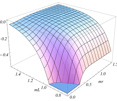
Figure 3: The topological part in the VEV of the energy density, $\langle T_{0}^{0}\rangle_{\text{t}}/m^{D+1}$, for a minimally coupled untwisted scalar field in 5-dimensional cosmic string spacetime with $q=3$, as a function of $mr$ and $mL$.

For a massless field the quantity $L^{D+1}\langle T_{i}^{j}\rangle_{\text{t}}$ is a function of the ratio $r/L$. In figure 4 we present the corresponding energy density (left panel) and the stress along the compact dimension (right panel) in the case of a $D=4$ minimally coupled scalar field for various values of the parameter $q$ (figures near the curves). The full/dashed curves correspond to untwsited/twisted scalar fields. In the case $q=1$ the cosmic string is absent and the corresponding VEVs are uniform. The graphs for a conformally coupled field are similar to those given in figure 4. Note that for the topological part in the vacuum effective pressure along the $j$-th direction we have (no summation) $p_{\text{t},j}=-$ $\langle T_{j}^{j}\rangle_{\text{t}}$, and, hence, for the example corresponding to figure 4 both the energy density and the pressure along the compact dimension are negative/positive for untwisted/twisted fields.

Figure 4: The topological parts in the VEV of the energy density (left panel) and the stress along the compact dimension, as functions of $r/L$ for a minimally coupled massless scalar field. The full and dashed curves correspond to untwisted and twisted fields, respectively. The figures near the curves are the values of the parameter $q$.

The topological parts in the radial and azimuthal stresses are plotted in figure 5 versus $r/L$ for minimally (full curves) and conformally (dashed curves) coupled untwisted fields in the geometry of a $D=4$ cosmic string with $q=2$. Note that the azimuthal stress is not a monotonic function in both cases. As it is seen, the corresponding effective pressures are positive. For a twisted field the graphs have similar structure with the signs changed.

Figure 5: The topological parts in the radial and azimuthal stresses for a $D=4$ minimally coupled massless field as a function of the ratio $r/L$ in the geometry of a $D=4$ cosmic string with $q=2$.

The dependence of the energy density on the parameter $\beta$ in the quasiperiodicity condition along the compact dimension is presented in figure 6 for a minimally coupled massless scalar field in $D=4$. The graphs are plotted for $r/L=0.3$ and for various values of $q$ (numbers near the curves). They are symmetric with respect to $\beta=1/2$.

Figure 6: The topological part in the VEV of the energy density for a $D=4$ minimally coupled massless field as a function of the phase parameter $\beta$ for $r/L=0.3$. The figures near the curves correspond to the values of $q$.

5 Vacuum energy

As we have seen before, the energy density corresponding to the pure string part diverges on the string as $1/r^{D+1}$. Consequently, the corresponding total vacuum energy is divergent. We can evaluate the total vacuum energy in the region $r\geqslant r_{0}>0$ per unit volume in the subspace $(x^{3},x^{4},\ldots,x^{D})$, defined as $E_{0,r\geqslant r_{0}}^{\text{(s)}}=\phi_{0}\int_{r_{0}}^{\infty}dr\,r\langle T_{0}^{0}\rangle_{\text{s}}$. By using the recurrence relation for the modified Bessel function and the formula (see [41]) $\int_{a}^{\infty}dx\,xf_{\nu}(x)=f_{\nu-1}(a)$, with the function $f_{\nu}(x)$ defined in (15), one finds

$$E_{0,r\geqslant r_{0}}^{\text{(s)}}=\frac{m^{D-1}\phi_{0}}{2(2\pi)^{(D+1)/2}}\left[\sum_{k=1}^{[q/2]}F(2mr_{0}s_{k},s_{k})-\frac{q\sin(q\pi)}{\pi}\int_{0}^{\infty}dy\frac{F(2mr_{0}\cosh(y),\cosh(y))}{\cosh(2qy)-\cos(q\pi)}\right],$$ (55)

with the notation

$$F(u,v)=\left(1-4\xi\right)u^{2}f_{(D+1)/2}(u)-f_{(D-1)/2}(u)/v^{2}.$$ (56)

For a massless field this formula is reduced to

$$E_{0,r\geqslant r_{0}}^{\text{(s)}}=\frac{\Gamma((D-1)/2)}{4(4\pi)^{(D-1)/2}qr_{0}^{D-1}}\left[\left(1-4\xi\right)(D-1)g_{D}(q)-g_{D+2}(q)\right].$$ (57)

Of course, this result could also be obtained directly from (47). For $mr_{0}\gg 1$ and for fixed value of $q$, the dominant contribution to (55) comes from the first term in the right hand side of Eq. (56) and the vacuum energy is positive for $\xi<1/4$. In particular, this is the case for both minimally and conformally coupled fields. In the case $mr_{0}\ll 1$, the leading term in the asymptotic expansion of the vacuum energy is given by (57). For large values of $q$ the second term in the square brackets of (57) dominates and the vacuum energy is negative with independence of the curvature coupling parameter. For $q\gtrsim 1$, the vacuum energy given by (57) remains negative for a conformally coupled field and becomes positive for a minimally coupled field.

Now we turn to the topological part of the vacuum energy. The corresponding energy-momentum tensor can be further decomposed as

$$\langle T_{i}^{j}\rangle_{\text{t}}=\langle T_{i}^{j}\rangle_{\text{t}}^{\text{(M)}}+\langle T_{i}^{j}\rangle_{\text{t}}^{\text{(s)}},$$ (58)

where the second term on the right hand side is the correction due to the presence of the string. The expression for $\langle T_{i}^{j}\rangle_{\text{t}}^{\text{(s)}}$ is obtained from (43) by subtracting the part corresponding to the term $k=0$ (the latter coincides with $\langle T_{i}^{j}\rangle_{\text{t}}^{\text{(M)}}$). For the correction in the topological part of the vacuum energy per unit volume in the subspace $(x^{4},\ldots,x^{D})$, induced by the string, we have

$$E_{\text{t}}^{\text{(s)}}=\int_{0}^{\infty}dr\,r\int_{0}^{\phi_{0}}d\phi\int_{0}^{L}dz\,\langle T_{0}^{0}\rangle_{\text{t}}^{\text{(s)}}.$$ (59)

By taking into account that $\langle T_{0}^{0}\rangle_{\text{t}}^{\text{(s)}}$ is given by the expression (43) omitting the $k=0$ term, the integral over $r$ is evaluated by using the formula [41]

$$\int_{a}^{\infty}dx\,x(x^{2}-a^{2})^{\beta-1}f_{\nu}(cx)=2^{\beta-1}c^{-2\beta}f_{\nu-\beta}(ac),$$ (60)

with the function $f_{\nu}(x)$ defined in Eq. (15). As a result, the dependence on the parameter $q$ is factorized in the form of $g_{3}(q)/q$, where the function $g_{D}(q)$ is given by (32). By taking into account the expression (34) for $g_{3}(q)$, we find the final expression for the vacuum energy:

$$E_{\text{t}}^{\text{(s)}}=-\frac{q^{2}-1}{6q}\frac{m^{D-1}L}{(2\pi)^{(D-1)/2}}\sum_{l=1}^{\infty}\cos(2\pi l\beta)f_{(D-1)/2}(lmL).$$ (61)

As it is seen, the total energy does not depend on the curvature coupling parameter. It is negative/positive for untwisted/twisted scalar fields.

For a massless field we find

$$E_{\text{t}}^{\text{(s)}}=\frac{q^{2}-1}{qL^{D-2}}h_{D}(\beta),$$ (62)

where

$$h_{D}(\beta)=-\frac{\Gamma((D-1)/2)}{12\pi^{(D-1)/2}}\sum_{l=1}^{\infty}\frac{\cos(2\pi l\beta)}{l^{D-1}}.$$ (63)

For a massive field, the expression (62) gives the leading term in the asymptotic expansion for $mL\ll 1$. For odd values of $D$, the series in (63) is given in terms of the Bernoulli polynomials:

$$h_{D}(\beta)=\frac{(-1)^{(D-1)/2}\pi^{D/2}}{12(D-1)\Gamma(D/2)}B_{D-1}(\beta).$$ (64)

In figure 7 we plotted the function $h_{D}(\beta)$ for $D=3,4,5$ (figures near the curves). As in the case of the vacuum densities, this function is symmetric with respect to $\beta=1/2$.

Figure 7: The function $h_{D}(\beta)$ in (62) for $D=3,4,5$ (figures near the curves).

6 Conclusion

In the present paper we have investigated the one-loop quantum effects for a massive scalar field with general curvature coupling parameter, induced by the compactification of spatial dimensions in a generalized cosmic string spacetime. It is assumed that along the compact dimension the field obeys quasiperiodicity condition with an arbitrary phase. As the first step for the investigation of vacuum densities we evaluate the positive frequency Wightman function. This function gives comprehensive insight into vacuum fluctuations and determines the response of a particle detector of the Unruh-DeWitt type in a given state of motion. For a massive field and for general value of the planar angle deficit, the Wightman function is given by formula (22). The $l=0$ term in this expression corresponds to the Wightman function in the geometry of a cosmic string without compactification and, hence, the topological part is explicitly extracted. As the compactification under consideration does not change the local geometry, in this way the renormalization for the VEVs in the coincidence limit is reduced to that for the standard cosmic string geometry without compactification. For integer values of the parameter $q$, the Wightman function is expressed as an image sum of the corresponding function in the Minkowski spacetime with a compact dimension and is given by Eq. (23).

The VEV of the field squared is decomposed as the sum of the pure string part and the correction due to the compactification. For a massive field the string part is given by (29). Since the geometry is locally flat, this part does not depend on the curvature coupling parameter. It is positive for $q>1$ and diverges on the string like $1/r^{D-1}$. This divergence may be regularized considering a more realistic model of the string with nontrivial inner structure. The topological part in the VEV of the field squared is given by the expression (35) and it is finite everywhere including the points on the string. In dependence of the value of the phase $\beta$ in the quasiperiodicity condition, this part can be either positive or negative. In particular, the topological part is positive for an untwisted scalar and it is negative for a twisted scalar. At distances from the string larger than the length of the compact dimension, the topological part in the VEV of the field squared approaches to the corresponding quantity in the Minkowski spacetime with a compact dimension. For points near the string we have the simple asymptotic relation $\langle\varphi^{2}\rangle_{\text{t}}\approx q\langle\varphi^{2}\rangle_{\text{t}}^{\text{(M)}}$.

The VEV of the energy-momentum tensor is investigated in section 4. This VEV is diagonal and, similar to the case of the field squared, it is decomposed into the pure string and topological parts, given by expressions (46) and (43), respectively. We have explicitly checked that the topological part satisfies the covariant conservation equation and its trace is related to the VEV of the field squared by the standard formula. For a massive field and for general value of the parameter $q$, we give a closed expression for the pure string part in the VEV of the energy-momentum tensor in arbitrary number of dimensions. The latter generalizes various special cases previously discussed in the literature. At large distances from the string, the topological part coincides with the corresponding result in the Minkowski spacetime and it dominates in the total VEV. In this limit the VEV of the energy-momentum tensor does not depend on the curvature coupling parameter and the corresponding energy density is negative/positive for untwisted/twisted scalar fields. The topological part is finite on the string and for points near the string the leading term in the corresponding asymptotic expansion is given by (53). The pure string part in the VEV of the energy density diverges on the string as $1/r^{D+1}$ and near the string it dominates in the total VEV. For a conformally coupled scalar field the corresponding energy density is negative, whereas for a minimally coupled field the energy density is positive for small values of the parameter $q$ and becomes negative for large values of $q$. The numerical examples are given for the simplest Kaluza-Klein-type model with a single extra dimension. They show that he nontrivial topology due to the cosmic string enhances the vacuum polarization effects induced by the compactness of spatial dimensions for both the field squared and the vacuum energy density. For a charged scalar field, in the presence of a constant gauge field the expression for the topological parts are obtained from the formulas given above by the replacement $\beta\rightarrow\beta^{\prime}$ with $\beta^{\prime}$ defined by (26). In this case the topological parts are periodic functions of the component of the gauge field along the compact dimension. This is an analog of the Aharonov-Bohm effect.

As a result of the non-integrable divergence of the energy density in the pure string part on the string, the corresponding total vacuum energy is divergent. In section  5 we give a closed expression, Eq. (55), for the vacuum energy in the region $r\geqslant r_{0}>0$. The topological part in the VEV of the energy-momentum tensor can be further decomposed into the Minkowskian and string induced parts. The latter is finite on the string and vanishes at large distances from the string. As a result, the total vacuum energy corresponding to this part is finite. This energy is given by the expressions (61) and (62) for massive and massless fields, respectively. In these expressions the dependence on the parameter $q$ is simply factorized. The string induced part in the topological energy does not depend on the curvature coupling parameter and it is negative/positive for untwisted/twisted scalars.

In a way similar to that described above, one can consider the topological Casimir effect for a cosmic string in de Sitter spacetime with compact spatial dimensions. The vacuum polarization effects induced by the presence of the string in uncompactified de Sitter spacetime have been recently discussed in Ref. [46]. The topological Casimir densities in de Sitter spacetime with toroidally compactified spatial dimensions are investigated in Ref. [47]. It has been shown that the curvature of the background spacetime decisively influences the behavior of the topological parts in the VEVs of the field squared and the energy density for lengths of compact dimensions larger than the curvature scale of the spacetime.

In this paper the string geometry is taken as a static, given classical background for quantum matter fields. This approach follows the main part of the papers where the influence of the string on quantum matter is investigated (see references [7]-[23]). Of course, in a more complete approach the dynamics of the cosmic string should be taken into account. In the simplest model, the cosmic string dynamics can be described by the Nambu action (see, for instance, [2]). If the scalar field under consideration interacts with the Higgs field inside the string core, then, within this model, the total action will contain also the term describing the interaction of the scalar field with the vibrational modes of the string. This would be the further development of the model under discussion. The results obtained in the present paper are the first step to this more general problem. Another development would be the investigation of the back-reaction effects of the quantum energy-momentum tensor on the gravitational field of the cosmic string. For the geometry of infinitely thin straight cosmic string the back-reaction for conformal fields has been discussed in [20, 48] by using the linearized semiclassical Einstein equations. It would also be interesting to generalize the vacuum polarization calculations of the present paper for the models with nontrivial string core. For a general cylindrically symmetric static model of the string core with finite support this can be done in a way similar to that used in [31] for the geometry of a straight cosmic string.

References

- [1] T.W.B. Kibble, Phys. Rep. 67, 183 (1980); A. Vilenkin, Phys. Rep. 121, 263 (1985).
- [2] A. Vilenkin and E.P.S. Shellard, Cosmic Strings and Other Topological Defects (Cambridge University Press, Cambridge, England, 1994).
- [3] T. Damour and A. Vilenkin, Phys. Rev. Lett. 85, 3761 (2000).
- [4] P. Bhattacharjee and G. Sigl, Phys. Rept. 327, 109 (2000).
- [5] V. Berezinsky, B. Hnatyk, and A. Vilenkin, Phys. Rev. D 64, 043004 (2001).
- [6] S. Sarangi and S.H.H. Tye, Phys. Lett. B 536, 185 (2002); E.J. Copeland, R.C. Myers, and J. Polchinski, JHEP 0406, 013 (2004); G. Dvali and A. Vilenkin, JCAP 03, 010 (2004).
- [7] T.M. Helliwell and D.A. Konkowski, Phys. Rev. D 34, 1918 (1986).
- [8] B. Linet, Phys. Rev. D 35, 536 (1987).
- [9] V.P. Frolov and E.M. Serebriany, Phys. Rev. D 35, 3779 (1987).
- [10] J.S. Dowker, Phys. Rev. D 36, 3095 (1987); J.S. Dowker, Phys. Rev. D 36, 3742 (1987).
- [11] P.C.W. Davies and V. Sahni, Class. Quantum Grav. 5, 1 (1988).
- [12] A.G. Smith, in The Formation and Evolution of Cosmic Strings, Proceedings of the Cambridge Workshop, Cambridge, England, 1989, edited by G.W. Gibbons, S.W. Hawking, and T. Vachaspati (Cambridge University Press, Cambridge, England, 1990).
- [13] G.E.A. Matsas, Phys. Rev. D 41, 3846 (1990).
- [14] B. Allen and A.C. Ottewill, Phys. Rev. D 42, 2669 (1990); B. Allen, J.G. Mc Laughlin, and A.C. Ottewill, Phys. Rev. D 45, 4486 (1992); B. Allen, B.S. Kay, and A.C. Ottewill, Phys. Rev. D 53, 6829 (1996).
- [15] T. Souradeep and V. Sahni, Phys. Rev. D 46, 1616 (1992).
- [16] K. Shiraishi and S. Hirenzaki, Class. Quantum Grav. 9, 2277 (1992).
- [17] V.B. Bezerra and E.R. Bezerra de Mello, Class. Quantum Grav. 11, 457 (1994); E.R. Bezerra de Mello, Class. Quantum Grav. 11, 1415 (1994).
- [18] G. Cognola, K. Kirsten, and L. Vanzo, Phys. Rev. D 49, 1029 (1994).
- [19] E.S. Moreira Jnr, Nucl. Phys. B 451, 365 (1995).
- [20] D. Iellici, Class. Quantum Grav. 14, 3287 (1997).
- [21] N.R. Khusnutdinov and M. Bordag, Phys. Rev. D 59, 064017 (1999).
- [22] V.B. Bezerra and N.R. Khusnutdinov, Class. Quantum Grav. 23, 3449 (2006).
- [23] M.E.X. Guimarães and B. Linet, Commun. Math. Phys. 165, 297 (1994); M.E.X. Guimarães, Class. Quantum Grav. 12, 1705 (1995); L. Sriramkumar, Class. Quantum Grav. 18, 1015 (2001); J. Spinelly and E.R. Bezerra de Mello, Class. Quantum Grav. 20, 873 (2003); Yu.A. Sitenko and N.D. Vlasii, Class. Quantum Grav. 26, 195009 (2009).
- [24] A.H. Castro Neto, F. Guinea, N.M.R. Peres, K.S. Novoselov, and A.K. Geim, Rev.Mod. Phys. 81, 109 (2009).
- [25] V.M. Mostepanenko and N.N. Trunov, The Casimir Effect and Its Applications (Oxford University Press, Oxford, 1997).
- [26] E. Elizalde, S.D. Odintsov, A. Romeo, A.A. Bytsenko, and S. Zerbini, Zeta Regularization Techniques with Applications (World Scientific, Singapore, 1994); K.A. Milton The Casimir Effect: Physical Manifestation of Zero-Point Energy (World Scientific, Singapore, 2002); M. Bordag, G. L. Klimchitskaya, U. Mohideen, and V.M. Mostepanenko, Advances in the Casimir Effect (Oxford University Press, Oxford, 2009).
- [27] H.B. Cheng, Phys. Lett. B 643, 311 (2006); H.B. Cheng, Phys. Lett. B 668, 72 (2008); S.A. Fulling and K. Kirsten, Phys. Lett. B 671, 179 (2009); K. Kirsten and S.A. Fulling, Phys. Rev. D 79, 065019 (2009); E. Elizalde, S.D. Odintsov, and A.A. Saharian, Phys. Rev. D 79, 065023 (2009); L.P. Teo, Phys. Lett. B 672, 190 (2009); L.P. Teo, Nucl. Phys. B 819, 431 (2009); L.P. Teo, JHEP 0906, 076 (2009); L.P. Teo, JHEP 0911, 095 (2009).
- [28] K. Poppenhaeger, S. Hossenfelder, S. Hofmann, and M. Bleicher, Phys. Lett. B 582, 1 (2004); A. Edery and V.N. Marachevsky, Phys. Rev. D 78, 025021 (2008); A. Edery and V.N. Marachevsky, JHEP 0812, 035 (2008); F. Pascoal, L.F.A. Oliveira, F.S.S. Rosa, and C. Farina, Braz. J. Phys. 38, 581 (2008); L. Perivolaropoulos, Phys. Rev. D 77, 107301 (2008).
- [29] S. Bellucci and A.A. Saharian, Phys. Rev. D 80, 105003 (2009); E. Elizalde, S.D. Odintsov, and A.A. Saharian, Phys. Rev. D 83, 105023 (2011).
- [30] I. Brevik and T. Toverud, Class. Quantum Grav. 12, 1229 (1995).
- [31] E.R. Bezerra de Mello, V.B. Bezerra, A.A. Saharian and A.S. Tarloyan, Phys. Rev. D 74, 025017 (2006).
- [32] E.R. Bezerra de Mello, V.B. Bezerra, and A.A. Saharian, Phys. Lett. B 645, 245 (2007); E. R. Bezerra de Mello, V. B. Bezerra, A. A. Saharian, and A. S. Tarloyan, Phys. Rev. D 78, 105007 (2008); G. Fucci and K. Kirsten, JHEP 1103, 016 (2011); E.R. Bezerra de Mello and A.A. Saharian, Class. Quantum Grav. 28, 145008 (2011); G. Fucci and K. Kirsten, J. Phys. A 44, 295403 (2011).
- [33] G.E. Volovik, Pisma Zh. Eksp. Teor. Fiz. 67, 666 (1998) [JETP Lett. 67, 698 (1998)].
- [34] A. Krishnan, et al, Nature 388, 451 (1997); S.N. Naess, A. Elgsaeter, G. Helgesen and K.D. Knudsen, Sci. Technol. Adv. Mater. 10, 065002 (2009).
- [35] E.R. Bezerra de Mello, V.B. Bezerra, A.A. Saharian, and V.M. Bardeghyan, Phys. Rev. D 82, 085033 (2010); S. Bellucci, E.R. Bezerra de Mello, and A.A. Saharian, Phys. Rev. D 83, 085017 (2011).
- [36] N.D. Birrell and P.C.W. Davies, Quantum Fields in Curved Space (Cambridge University Press, Cambridge, England, 1982).
- [37] S. Tagaki, Prog. Theor. Phys. Suppl. 88, 1 (1986).
- [38] S. Bellucci, A.A. Saharian, and V.M. Bardeghyan, Phys. Rev. D 82, 065011 (2010).
- [39] A.A. Saharian, The Generalized Abel-Plana Formula with Applications to Bessel Functions and Casimir Effect (Yerevan State University Publishing House, Yerevan, 2008); Report No. ICTP/2007/082; arXiv:0708.1187.
- [40] A.A. Saharian, Proceedings of Science PoS(IC2006)019, hep-th/0609093.
- [41] A.P. Prudnikov, Yu.A. Brychkov, and O.I. Marichev, Integrals and Series (Gordon and Breach, New York, 1986), Vol. 2.
- [42] G.N. Watson, A Treatise on the Theory of Bessel Functions (Cambridge University Press, Cambridge, 1944).
- [43] M. Abramowitz and I.A. Stegun, Handbook of Mathematical Functions (Dover, New York, 1972).
- [44] J. Spinelly and E.R. Bezerra de Mello, JHEP 0812, 081 (2008).
- [45] A.A. Saharian, Phys. Rev. D 69, 085005 (2004).
- [46] E.R. Bezerra de Mello and A. A. Saharian, JHEP 0809, 005 (2008).
- [47] A.A. Saharian and M.R. Setare, Phys. Lett. B 659, 367 (2008); S. Bellucci and A.A. Saharian, Phys. Rev. D 77, 124010 (2008); A.A. Saharian, Class. and Quantum Grav. 25, 165012 (2008); E.R. Bezerra de Mello and A.A. Saharian, JHEP 0812, 081 (2008).
- [48] W.A. Hiscock, Phys. Lett. B 188, 317 (1987); M.E.X. Guimarães, Phys. Lett. B 398, 281 (1997); V.A. De Lorenci and E.S. Moreira Jr, Phys. Lett. B 679, 510 (2009).