Abstract

When brain signals are recorded in an electroencephalogram or some similar large-scale record of brain activity, oscillatory patterns are typically observed that are thought to reflect the aggregate electrical activity of the underlying neuronal ensemble. Although it now seems that such patterns participate in feedback loops both temporally with the neurons’ spikes and spatially with other brain regions, the mechanisms that might explain the existence of such loops have remained essentially unknown. Here we present a theoretical study of these issues on a cortical model we introduced earlier [Nathan A, Barbosa VC (2010) Network algorithmics and the emergence of the cortical synaptic-weight distribution. Phys Rev E 81: 021916]. We start with the definition of two synchronization measures that aim to capture the synchronization possibilities offered by the model regarding both the overall spiking activity of the neurons and the spiking activity that causes the immediate firing of the postsynaptic neurons. We present computational results on our cortical model, on a model that is random in the Erdős-Rényi sense, and on a structurally deterministic model. We have found that the algorithmic component underlying our cortical model ultimately provides, through the two synchronization measures, a strong quantitative basis for the emergence of both types of synchronization in all cases. This, in turn, may explain the rise both of temporal feedback loops in the neurons’ combined electrical activity and of spatial feedback loops as brain regions that are spatially separated engage in rhythmic behavior.

Introduction

Current technology allows the recording of electromagnetic brain activity at several different spatial scales, ranging from invasive recordings that capture the signals from neuronal ensembles comprising thousands to millions of cells to those that are noninvasive (like the electroencephalogram) and capture the signals from large-scale cortical areas [1]. Invariably the recorded signals appear as oscillatory patterns which, depending on the scale at which the recording is performed, occur in different frequency ranges and provide distinct interpretive possibilities. At the smallest spatial scales, for example, the recorded signals occur in the range of a few kilohertz and are thought to reflect the combined spiking (or firing) activity of the group of neurons in question. The signals recorded at the largest scales, on the other hand, occur in the range of a few to $100$ hertz and are thought to reflect the so-called local field potentials (LFPs), which in turn are purported to reflect the aggregate effects of all the electrical activity taking place in the corresponding area [2].

LFPs have acquired great prominence recently, owing mainly to the fact that LFPs related to different brain areas appear to combine with one another in such ways as to correlate significantly with the brain’s sensory-motor mechanisms and other, higher-level functions as well (such as memory, attention, and others; cf. [3, 4, 5] and references therein). The ways in which LFPs combine seem to involve forms of cross-frequency coupling that cover wide temporal and spatial ranges and ultimately promote the integration of activities with different temporal and spatial characteristics [5]. Decoding the various forms of LFP coupling may one day hold the key to understanding how computation and communication take place in the brain.

As it happens, though, many aspects of the nature of LFPs have remained elusive. In particular, their precise origin and relation to the underlying firing activity of the neurons seem to depend crucially on the brain region being considered. However, notwithstanding this indefiniteness that still surrounds the specifics of LFP emergence and interaction with other LFPs, some of the crucial points are beginning to be clarified [6, 2]. One of them is the relation with the combined firing activity of groups of neurons. Although LFPs seem to derive largely from the accumulation of potential at the neurons’ membranes that eventually leads to neuronal firing, it appears that the firing patterns themselves have a role to play as well. As a consequence, a picture that seems to be emerging is that of a feedback loop in which the larger-scale LFPs both influence and get influenced by the smaller-scale firing patterns. Another point is more related to the spatial characteristics of how LFPs interact with one another: It now seems clear that feedback loops also occur involving the LFPs of distinct brain areas.

While a complete resolution of these issues will certainly require considerable further research, a detailed understanding will undoubtedly benefit from a clear picture of firing synchronization at the neuronal level. By synchronization we mean both the convergence of multiple action potentials onto distinct cells within a relatively narrow temporal window, and also the firing due to such potentials within a similar window. As we mentioned above, both phenomena are closely related to the rise of LFPs, and consequently the rise of the higher-level functions that LFPs are thought to support. In our view, accounting for the possibilities the brain affords for the appearance of such synchronized behavior depends both on the anatomical properties of how neurons interconnect and on the individual firing behavior of each neuron. Our aim in this paper is the study of these types of synchronism on a graph-theoretic model of the cortex.

Our study is preceded by a few others [7, 8, 9], all of which have modeled neuronal behavior as a continuous-time process in which the relevant signals obey certain differential equations and feed some measure of synchronous activity. Invariably these studies have modeled the synchronization of membrane potentials directly, and have for this reason stayed apart from explicitly modeling most of the relevant details that characterize neuronal firings, like the so-called local histories of each neuron [10]. Our approach is to take a different course and focus on the extent to which certain events at the various neurons can be said to be synchronized. These events are, in essence, the arrival of action potentials from other neurons and the eventual creation of new action potentials. These, of course, are precisely the events that make up membrane potentials, but we have found in previous studies of related problems that the additional level of detail pays off by providing unprecedented insight. Examples here are the emergence of the synaptic-weight distribution, in which case we demonstrated that experimentally observed distributions [11] can be reproduced [12], and a more tractable version [13] of the integrated-information theory for the emergence of consciousness [14].

Our model is based on what is generally called network algorithmics. In our case this refers to the combination of a structural component to represent the anatomical properties of the cortex at the neuronal level, and a distributed-algorithmic component to represent the traffic of action potentials among the neurons as they fire. In general, a distributed algorithm is a collection of sequential procedures, each run by an agent in a distributed system with provisions for messages to be sent to other agents for communication [15]. The distributed algorithm of interest here is inherently asynchronous, meaning that the behavior of each agent (each neuron) is purely reactive to the arrival of messages (action potentials), which can in turn undergo unpredictable delays before delivery. It follows that independent runs of the same algorithm from the same initial conditions cannot in general be guaranteed to generate the same sequence of message arrivals at any agent, and therefore not the same behavior. Lately, this inherent source of unpredictability has led asynchronous distributed algorithms to be recognized as a powerful abstraction in the modeling of biological systems [16, 17], since they allow the incorporation into the model of small behavioral variations that might otherwise be simply smoothed out and rendered irrelevant.

An asynchronous distributed algorithm never makes any reference to a global-time entity. In our model, therefore, every property emerging from neuronal interactions is the result of strictly local elements. The presence of such strong asynchronism may seem contradictory with the search for signs of synchronism. However, we have found that observing the system from the outside can reveal surprising synchronization possibilities that could never be known within the scope of individual neurons, provided we uncover the causal relationship that binds those local elements on a global scale.

Using network algorithmics as the basis of our model makes it substantially more detailed than those that target membrane potentials as the basic analytical units, in the sense that a neuron’s behavior can now be described as its reaction to the arrival of a new action potential given its current state. Clearly, though, there would be room for considerably more detail, even down to the molecular level. Our approach, therefore, resides in the middle ground between two extremes and as such is related to what has become known as the artificial-life approach [18, 19], whose “life as it could be” metaphor is close in spirit to our own view. Our approach is also part of a growing collection of efforts that attempt to tackle eminent problems of neuroscience from the perspective of graph-based and other interdisciplinary methods [20, 21, 22, 23, 24, 25, 26, 27, 28, 29, 30, 31]. As an enterprise that eventually seeks to be able to handle realistically large problem instances from a graph-theoretic perspective, the present study is moreover in line with the many others that in the last decade have addressed the so-called complex networks [32, 33, 34].

Our model is defined on a strongly connected directed graph $S$, i.e., a directed graph in which it is possible to reach every node from every other node through directed paths only. We assume that $S$ has $N$ nodes, each representing a neuron, so each one can be either excitatory or inhibitory in the proportion of $4$ to $1$, respectively [35, 36, 37]. In $S$, an edge exists directed from node $i$ to node $j$ to indicate a synapse from $i$’s axon to one of $j$’s dendrites, but no edge can connect two inhibitory nodes [35]. The results we describe in the remainder of the paper for our cortical model are predicated upon $S$ being drawn from the following random-graph model on $n\geq N$ nodes in such a way that $S$ is the giant strongly connected component, GSCC [38], of the directed graph $D$ that is actually drawn. In $D$ a randomly chosen node, say $i$, has out-degree $k>0$ with probability proportional to $k^{-1.8}$. Following [50, 51], each of these $k$ nodes is precisely another randomly chosen node, say $j$, with probability proportional to $e^{-d_{ij}}$, where $d_{ij}$ is the Euclidean distance between nodes $i$ and $j$ when all $n$ nodes are placed uniformly at random on a radius-$1$ sphere. We have observed this policy for edge placement to lead to $N\approx 0.9n$ on average (i.e., we expect the GSCC of $D$, and hence $S$, to comprise roughly $90\%$ of the $n$ nodes) [13].

Methods

We start with the specification of the asynchronous distributed algorithm to be executed by the nodes of graph $S$. This algorithm prescribes a common procedure for each node to react to the arrival of a message and to possibly send messages out as a consequence. Such a procedure runs atomically (i.e., without being interrupted), so actually implementing the algorithm requires provisions for the queuing of incoming messages at each node. Each run of the distributed algorithm can be described formally by specifying how the various message arrivals at the different nodes relate to one another. As we do this a precise notion of causality emerges and we use it to define our two synchronization measures.

Asynchronous distributed algorithm

All nodes in $S$ share the same rest and threshold potentials, denoted by $v^{0}$ and $v^{\mathrm{t}}$, respectively, such that $v^{0}<v^{\mathrm{t}}$. We use $v_{j}$ to represent the potential of node $j$ and $w_{ij}$ to represent the synaptic weight of the edge directed from $i$ to $j$. At all times, these are constrained in such a way that $v_{j}\in[v^{0},v^{\mathrm{t}}]$ and $w_{ij}\in[0,1]$. An asynchronous distributed algorithm, henceforth referred to as $A$, underlies the node-potential and synaptic-weight dynamics of our cortical model. At node $j$, algorithm $A$ is built around the “firing” operation which consists of sending a message to each out-neighbor of $j$ in $S$ and setting $v_{j}$ to the rest potential $v^{0}$. Algorithm $A$ is purely reactive, that is, it only acts at any node when the node receives a message. Evidently there must be exceptions to this purely reactive character, since at least one node must send messages out spontaneously to start the algorithm. We call such nodes initiators and let $m\leq N$ be the number of initiators in a given run of algorithm $A$. When node $j$ acts as an initiator (this happens at most once in a run for that node), it simply fires with probability $1$. When it reacts to the reception of a message, say from node $i$, node $j$ performs the following steps:

1. If $i$ is excitatory, then set $v_{j}$ to $\min\{v^{\mathrm{t}},v_{j}+w_{ij}\}$. If it is inhibitory, then set $v_{j}$ to $\max\{v^{0},v_{j}-w_{ij}\}$.

2. Fire with probability $(v_{j}-v^{0})/(v^{\mathrm{t}}-v^{0})$.

3. If firing did occur during step 2, then set $w_{ij}$ to $\min\{1,w_{ij}+\delta\}$. If it did not occur but the previous message received by node $j$ from any of its in-neighbors did cause firing to occur, then set $w_{ij}$ to $(1-\alpha)w_{ij}$.

The parameters $\delta$ and $\alpha$ appearing in step 3 are constrained by $\delta\leq\alpha$ [12]. They are meant to reproduce, although to a limited extent, the spike-timing-dependent plasticity principles [52, 53], which roughly dictate that $w_{ij}$ is to increase if firing occurs and decrease otherwise, always taking into account how close in time the relevant firings by nodes $i$ and $j$ are. Moreover, increases in $w_{ij}$ are to occur by a fixed amount, decreases by proportion [54, 55, 56]. Every run of algorithm $A$ is guaranteed to eventually reach a point at which no more message traffic exists. It is then said to have terminated.

Modeling causality

The problem of handling synchronization during a run of an asynchronous distributed algorithm such as algorithm $A$ is akin to that of handling simultaneity in special relativity. This is so because, in either context, establishing the notion of simultaneity is dependent upon how signals propagate and also on locality considerations [57]. A convenient framework within which to tackle it is then the event-based formalism originally laid down in [58]. An event in the present context is said to have occurred either when an initiator fires (and thereby sends a message to each of its out-neighbors in graph $S$) or when a node reacts to the reception of a message by executing steps 1–3 (which includes the possibility of firing). In either occasion the event involves the execution of an atomic set of actions by the node in question.

A run of algorithm $A$ can then be regarded as a set $R$ of events. An event $r\in R$ is described by the $4$-tuple $r=\langle i,t_{i},m_{i},M_{i}\rangle$, where $i$ identifies the node of $S$ at which event $r$ occurred, $t_{i}\geq 1$ indicates that $r$ was the $t_{i}$th event to occur at node $i$ since the run began, $m_{i}$ is the message (if any) that triggered the occurrence of the event, and $M_{i}$ is the set of messages sent by node $i$ if it fired during the event. Many of the events in $R$ are implicitly related to one another. We make such a relation explicit by defining the binary relation $B\subseteq R^{2}$. Given events $r$ as above and $r^{\prime}=\langle j,t_{j},m_{j},M_{j}\rangle$, we say that the ordered pair $(r,r^{\prime})\in B$ if and only if:

1. Either $i$ and $j$ are the same node and $t_{i}<t_{j}$ with no intervening event between $r$ and $r^{\prime}$;

2. Or $j$ is an out-neighbor of $i$ and $m_{j}\in M_{i}$ (i.e., the message that triggered $r^{\prime}$ was sent in connection with the occurrence of $r$).

We interpret $(r,r^{\prime})\in B$ as meaning that $r$ happened at node $i$ immediately before $r^{\prime}$. If (a) is the case, then this use of “before” seems natural because both $t_{i}$ and $t_{j}$ are relative to the same (local) time basis. Extending this interpretation to case (b), though apparently less natural, is still consistent because there is no reference in this case to either $t_{i}$ or $t_{j}$. Closing $B$ under transitivity yields another binary relation on $R$, here denoted by $B^{+}$, such that $B\subseteq B^{+}\subseteq R^{2}$. This relation can be interpreted in such a way that $(r,r^{\prime})\in B^{+}$ means that $r$ happened before $r^{\prime}$ regardless of how close the specific nodes at which they occurred are to each other in graph $S$. Through $B^{+}$, therefore, relation $B$ is the core of a characterization of how the events of run $R$ relate to one another causally. In particular, if $r$ and $r^{\prime}$ are such that neither $(r,r^{\prime})\in B^{+}$ nor $(r^{\prime},r)\in B^{+}$, then the situation is analogous to the space-like separation of events in special relativity (since neither could the occurrence of $r$ influence that of $r^{\prime}$ during run $R$, nor conversely).

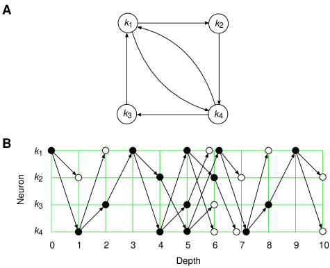
Figure 1: Directed graphs $S$ and $P$. A run of algorithm $A$ on graph $S$ (A) started by the single initiator $k_{1}$ may result in the set of events shown in panel B as the node set of graph $P$. Events are shown in panel B either as filled circles, in the case of firing events, or as empty circles, otherwise. Each event is positioned against a background grid that highlights the node of $S$ at which it occurred (this is given by the grid’s rows) and its depth (the grid’s columns). An edge of $P$ either joins consecutive events occurring at the same node of $S$ or corresponds to a message. We omit the former from panel B for clarity. An event’s depth is the greatest number of message edges on a directed path arriving at it. Every event (except the first one at the initiator) has exactly one incoming message edge. If it is a firing event, then it also has as many outgoing message edges as the corresponding node in graph $S$ has out-neighbors. Whenever two or more events occurring at the same node of $S$ have the same depth, they are shown as close to the correct grid point as possible.

Relation $B$ is also instrumental in our characterization of synchronization in run $R$. The first step is to recognize that it naturally gives rise to a directed graph, call it $P$, whose node set is $R$ (the set of events) and whose edge set is $B$. This graph is necessarily acyclic (no directed cycles are formed) and allows the definition of event $r$’s depth, denoted by $\mathit{depth}(r)$, as follows. Given a directed path in graph $P$ between two events, let the path’s length be defined as the number of edges on the path that correspond to messages. That is, the edges contributing to the path’s length are those that fall under case (b) above in the definition of relation $B$. We define $\mathit{depth}(r)$ as the length of the lengthiest path leading to $r$ in graph $P$. Intuitively, $\mathit{depth}(r)$ is the size of the longest causal chain of messages leading up to event $r$ during run $R$. These notions are illustrated in Figure 1.

Measures of synchronization

We use two measures of synchronization. They are both based on the premise that, if the sequence of events at two neurons (nodes of $S$) can be aligned with each other so that sufficiently many event pairs of the same depth become matched in the alignment, then there is more synchronism between the two sequences than there would be with fewer event pairs aligned. We do this sequence alignment as described next. Let $i$ and $j$ be the two neurons in question and let their event sequences during run $R$ be $e_{i}^{1},e_{i}^{2},\ldots,e_{i}^{L_{i}}$ and $e_{j}^{1},e_{j}^{2},\ldots,e_{j}^{L_{j}}$, respectively, where $L_{i}$ and $L_{j}$ are the sequences’ sizes. Let $\mu_{ij}=\max\{\mathit{depth}(e_{i}^{L_{i}}),\mathit{depth}(e_{j}^{L_{j}})\}$, i.e., $\mu_{ij}$ is the depth of the last event of the two sequences that is deepest. We do the alignment of the two sequences by creating two new size-$\mu_{ij}$ sequences, viz. $t_{1},t_{2},\ldots,t_{\mu_{ij}}$ and $u_{1},u_{2},\ldots,u_{\mu_{ij}}$ for the first measure, and $x_{1},x_{2},\ldots,x_{\mu_{ij}}$ and $y_{1},y_{2},\ldots,y_{\mu_{ij}}$ for the second measure, each with defining characteristics that depend on the particular measure of synchronization under consideration.

The first measure aims to capture the synchronization that may exist in the overall flow of messages and, through it, in the accumulation of potential at the neurons’ membranes. As such, it is based on positioning, relative to the $t$ sequence, those of the $L_{i}$ events of neuron $i$ that promoted the accumulation of potential, and likewise the $L_{j}$ events of neuron $j$ relative to the $u$ sequence. For $k=1,2,\ldots,\mu_{ij}$, the $t$ sequence is defined recursively as follows. If $k=1$:

• $t_{k}=1$, if $\mathit{depth}(e_{i}^{1})=1$;

• $t_{k}=0$, otherwise.

If $k>1$:

• $t_{k}=k$, if $\mathit{depth}(e_{i}^{\ell})=k$ for some $\ell\in\{1,2,\ldots,L_{i}\}$;

• $t_{k}=t_{k-1}$, otherwise.

The $u$ sequence is defined entirely analogously for neuron $j$.

If, for example, the events in the two original sequences have depths $2,3,3,7,8,9,11$ and $1,3,4,5,5,9$ for $i$ and $j$, respectively, then the $t$ sequence is

$$t=\langle 0,2,3,3,3,3,7,8,9,9,11\rangle$$ (1)

and the $u$ sequence is

$$u=\langle 1,1,3,4,5,5,5,5,9,9,9\rangle.$$ (2)

Thus, the $k$th position of sequence $t$ or $u$ equals $k^{\prime}$ such that $0<k^{\prime}\leq k$ if and only if the corresponding neuron received at least one message of depth $k^{\prime}$ during the run and, for $k^{\prime}<k$, never since did the neuron receive a message whose depth is in the interval $[k^{\prime}+1,k]$. It equals $0$ otherwise.

The first measure of synchronization is denoted by $\rho_{ij}^{-}$ for neurons $i$ and $j$. It is given by

$$\rho_{ij}^{-}=\frac{1}{\mu_{ij}}\sum_{k=1}^{\mu_{ij}}\frac{\min\{t_{k},u_{k}\}}{\max\{t_{k},u_{k}\}}$$ (3)

(assuming $0/0\equiv 1$). Clearly, $\rho_{ij}^{-}\in[0,1]$ and grows with the similarity of sequences $t$ and $u$. For identical sequences we get $\rho_{ij}^{-}=1$. The example above yields

$$\rho_{ij}^{-}=\frac{1}{11}\left(\frac{0}{1}+\frac{1}{2}+\frac{3}{3}+\frac{3}{4}+\frac{3}{5}+\frac{3}{5}+\frac{5}{7}+\frac{5}{8}+\frac{9}{9}+\frac{9}{9}+\frac{9}{11}\right)\approx 0.69.$$ (4)

The second measure addresses the synchronization possibilities that may exist as the neurons fire. In this case only those of the $L_{i}$ events of neuron $i$ that entailed firing are positioned relative to the $x$ sequence, and likewise the $L_{j}$ events of neuron $j$ with respect to the $y$ sequence. For $k=1,2,\ldots,\mu_{ij}$, the $x$ sequence is such that:

• $x_{k}=k$, if $\mathit{depth}(e_{i}^{\ell})=k$ for some $\ell\in\{1,2,\ldots,L_{i}\}$ such that neuron $i$ fired at the occurrence of $e_{i}^{\ell}$;

• $x_{k}=0$, otherwise.

The $y$ sequence is defined analogously for neuron $j$.

Following up on the examples given above, and assuming that neuron $i$ fired at one of its depth-$3$ events and neuron $j$ fired at all its events except those of depth $5$, the $x$ sequence is

$$x=\langle 0,0,3,0,0,0,0,0,0,0,0\rangle$$ (5)

and the $y$ sequence is

$$y=\langle 1,0,3,4,0,0,0,0,9,0,0\rangle.$$ (6)

Thus, the $k$th position of sequence $x$ or $y$ equals $k>0$ if and only if the corresponding neuron fired upon receiving a depth-$k$ message. It equals $0$ otherwise.

For neurons $i$ and $j$, the second measure of synchronization is denoted by $\rho_{ij}^{+}$ and given by

$$\rho_{ij}^{+}=\frac{1}{\mu_{ij}}\sum_{k=1}^{\mu_{ij}}\frac{\min\{x_{k},y_{k}\}}{\max\{x_{k},y_{k}\}}$$ (7)

(assuming $0/0\equiv 1$). As in the previous case, $\rho_{ij}^{+}\in[0,1]$ and grows with the similarity of sequences $x$ and $y$. Identical sequences yield $\rho_{ij}^{+}=1$. For the example above we get

$$\rho_{ij}^{+}=\frac{1}{11}\left(\frac{0}{1}+\frac{0}{0}+\frac{3}{3}+\frac{0}{4}+\frac{0}{0}+\frac{0}{0}+\frac{0}{0}+\frac{0}{0}+\frac{0}{9}+\frac{0}{0}+\frac{0}{0}\right)\approx 0.73.$$ (8)

For a fixed pair $i,j$ of neurons, both $\rho_{ij}^{-}$ and $\rho_{ij}^{+}$ seek to characterize the possibility of synchronized behavior during run $R$. They do this by quantifying the extent to which the events occurring at the two neurons could be said to happen synchronously if a time basis existed common to neurons $i$ and $j$ and time according to this basis elapsed along increasing event depth. Of course, our cortical model per se has no need for such a time basis and is algorithmically correct regardless of any timing assumptions one may make concerning the delay for action-potential propagation down the axons. However, the kind of synchronized behavior we are investigating occurs at a variety of temporal and spatial scales, therefore some time-related assumption is inevitable if we are to extract any meaning out of the multitude of neuronal events. Our choice seems reasonable because, conceptually, it contrasts with the algorithm’s inherent asynchronism only minimally: Every single pair of neurons is given its own time basis for the computation of $\rho_{ij}^{-}$ and $\rho_{ij}^{+}$ and this is reflected on the notationally explicit dependency of $\mu_{ij}$ on the $i,j$ pair. Furthermore, viewing increasing event depth as time may even have some biological plausibility to it. In fact, it appears that the delay for an action potential to reach the various synapses connecting out of the same axon is independent of how much of the axon actually has to be traversed [59, 60]. In these terms, what our assumption does is to generalize this independence for a group of axons.

Notwithstanding this common underlying feature of the two synchronization measures, they are also markedly different in how they use event depth to assess the similarity of two event sequences. In the case of $\rho_{ij}^{+}$, this is done rather stringently, since only same-depth firing events and the $0/0$ ratios contribute to it. In the case of $\rho_{ij}^{-}$, these continue to be some of the strongest contributors, but now they are joined by any pair of same-depth events (not necessarily firing ones). Moreover, now an event’s depth lingers until a greater-depth event occurs and in the meantime continues to influence $\rho_{ij}^{-}$.

Results

Our computational results are based on the same methodology we followed in [13], of which we now provide a brief review for the reader’s benefit. We use $v^{0}=-15$, $v^{\mathrm{t}}=0$, $\delta=0.0002$, and $\alpha=0.04$ in all runs of algorithm $A$ on $S$. Each run starts at $m=50$ initiators chosen uniformly at random and progresses until termination. A run is implemented as a sequential program that, initially, selects an initiator randomly out of the $m$ that were chosen for the run, lets it fire, and queues up the messages it sends for reception by the destination nodes. Subsequently, after all initiators have had a chance to proceed in this way, a list is maintained containing all nodes with nonempty input-message queues. One of them is selected at random and the processing of its head-of-queue message is carried out (again with the possible queuing of messages for consumption by other nodes). This is repeated until all queues are empty.

The directed graph $S$ can be of one of types (i)–(iii), as explained next. In order to keep the computational effort reasonably bounded with current technology, the directed graph $D$ of which $S$ is the GSCC has $n=100$ nodes.

• In this case $D$ is sampled from the cortical model described above. As explained, the corresponding $S$ is expected to have $N\approx 90$ nodes. The expected in- or out-degree in $D$ is $3.7$.

• In this case $D$ is sampled from the generalized Erdős-Rényi model of directed graphs [61]. Given the expected in- or out-degree $z$, an edge is placed from each node $i$ to each node $j\neq i$ with probability $z/(n-1)$. For consistency with type-(i) graphs we use $z=3.7$, in which case $S$ is such that $N\approx 100$ with high probability.

• In this case $D$ has a deterministic structure and is by construction strongly connected. So $S=D$ and $N=100$. The structure of $D$ is that of the directed circulant graph [62] with in- or out-degree equal to $\lceil 3.7\rceil=4$. If we number the $n$ nodes $0,1,\ldots,n-1$, then in $D$ every node $i$ has nodes $i+1$, $i+2$, $i+3$, and $i+4$ (modulo $n$) as out-neighbors.

For each fixed $S$, $0.2N$ nodes are chosen uniformly at random to be inhibitory, so long as no two of these nodes are connected by an edge [note that, if $S$ is of type (iii), then all $20$ inhibitory nodes are in fact placed deterministically, since necessarily they are found at equal intervals as we traverse the nodes in the order $0,1,\ldots,n-1$]. Moreover, for each $S$ node potentials and synaptic weights are chosen uniformly at random from the intervals $[v^{0},v^{\mathrm{t}}]$ and $[0,1]$, respectively. For type-(iii) graphs this is the only source of nondeterminism.

We use $50$ $S$ instances of each type. For each fixed $S$ we use $50\,000$ run sequences of algorithm $A$, each sequence comprising $10\,000$ runs. The first run in a sequence starts from the node potentials and synaptic weights chosen for the graph. Each subsequent run in the sequence starts from the node potentials and synaptic weights at which the previous run ended. Along each sequence we observe the behavior of $\rho_{ij}^{-}$ and $\rho_{ij}^{+}$ for each pair $i,j$ of distinct nodes at six checkpoints. The first of these occurs before any run actually takes place. Each of the remaining five occurs after $2\,000$ additional runs have elapsed. The observation that takes place at a checkpoint is based on $100$ additional runs, called side runs, each starting at its own set of $m$ randomly chosen initiators and from the node potentials and synaptic weights that are current at the checkpoint. At the end of the side runs, the main sequence of runs is resumed from these same node potentials and synaptic weights.

It is important to note that this computational setup would entail a considerable amount of processing even if the side runs were excluded, since for fixed $S$ algorithm $A$ would be run to completion $5\times 10^{8}$ times. These runs are grouped into sequences so that the cumulative action of the model’s weight-update rule can be effected, but we also need many independent sequences to account for the inherent nondeterminism of our model’s asynchronous setting. As defined, however, our synchronization measures are properties of a single run, so they too need to be averaged out over many runs. We might have chosen to do so directly over the runs that correspond to checkpoints, that is, over $50\,000$ runs per checkpoint (one for each sequence). Each of these runs, however, starts at the set of node potentials and synaptic weights that are current in its sequence, so for each such set only one run would take place. Introducing side runs has been a means to increase this number to $100$, with the consequence of elevating the overall number of runs for fixed $S$ to $5.3\times 10^{8}$.

The contribution of each side run concerning a fixed pair $i,j$ of distinct nodes is to record the values of $\rho_{ij}^{-}$ and $\rho_{ij}^{+}$ at the end of the run, as well as tag them with the labels $\delta_{\mathrm{min}}=\min\{\delta_{ij},\delta_{ji}\}$ and $\delta_{\mathrm{max}}=\max\{\delta_{ij},\delta_{ji}\}$, where $\delta_{ij}$ and $\delta_{ji}$ are the directed distances between the two nodes in $S$ (from $i$ to $j$ and from $j$ to $i$, respectively). After all $2.5\times 10^{8}$ side runs for a graph type have been completed at a checkpoint, we calculate the average values of $\rho_{ij}^{-}$ and $\rho_{ij}^{+}$ over all node pairs having the same tags. These averages are henceforth denoted by $\rho^{-}$ and $\rho^{+}$, respectively.

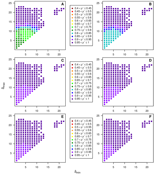
Figure 2: Average value of $\rho_{ij}^{-}$ for type-(i) graphs as a function of $\delta_{\mathrm{min}}$ and $\delta_{\mathrm{max}}$. Data are given for the first checkpoint (A) through the sixth (F).

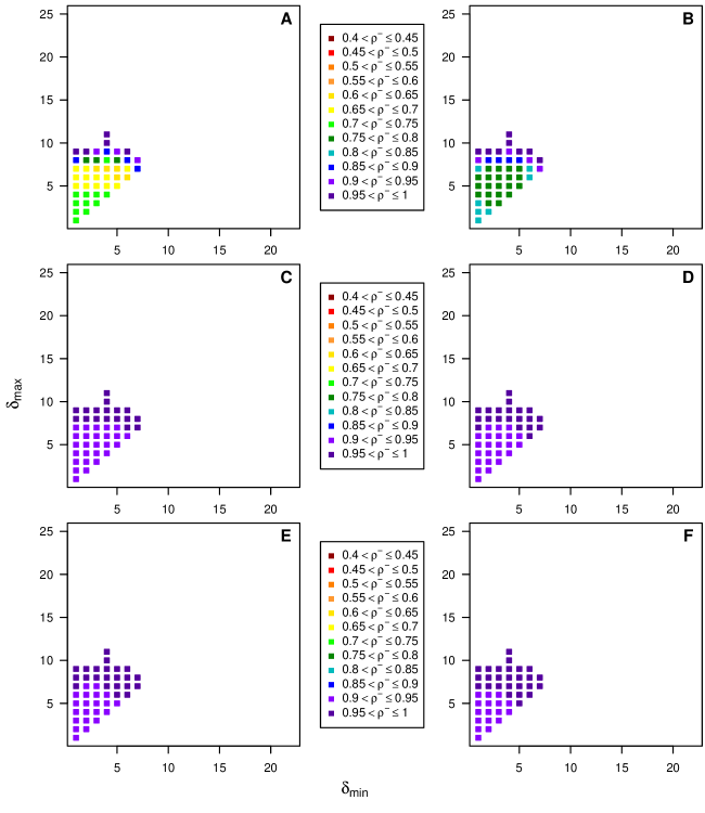
Figure 4: Average value of $\rho_{ij}^{-}$ for type-(ii) graphs as a function of $\delta_{\mathrm{min}}$ and $\delta_{\mathrm{max}}$. Data are given for the first checkpoint (A) through the sixth (F).

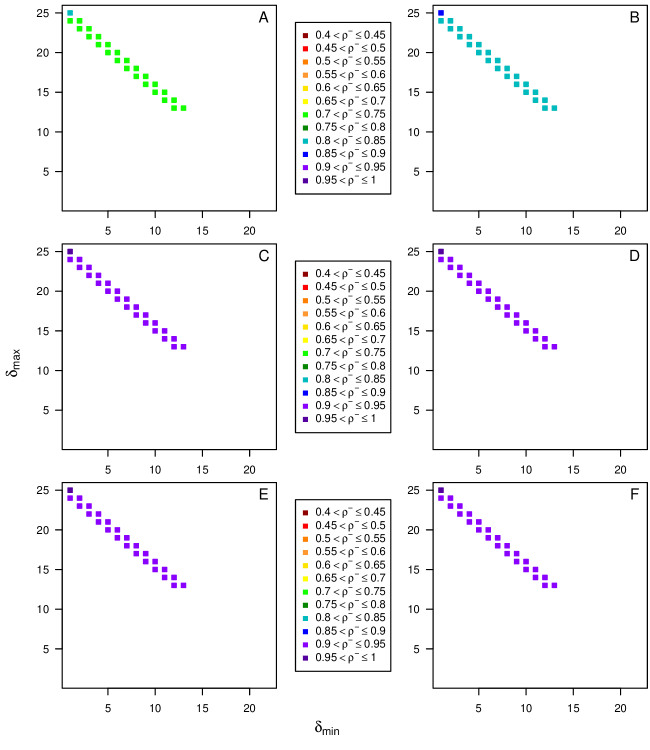
Figure 6: Average value of $\rho_{ij}^{-}$ for type-(iii) graphs as a function of $\delta_{\mathrm{min}}$ and $\delta_{\mathrm{max}}$. Data are given for the first checkpoint (A) through the sixth (F).

Our results are presented in Figures 2 and 3 for type-(i) graphs, Figures 4 and 5 for type-(ii) graphs, and Figures 6 and 7 for type-(iii) graphs. The former figure in each pair refers to $\rho^{-}$, the latter figure to $\rho^{+}$. Each figure comprises six panels, each panel for each of the six observational checkpoints. The A panels refer to the first checkpoints, the B panels to the second checkpoints, and so on. Each panel is organized as a two-dimensional array and gives the $\rho^{-}$ or $\rho^{+}$ averages as a function of the node pairs’ $\delta_{\mathrm{min}}$ values (as abscissas) and $\delta_{\mathrm{max}}$ values (as ordinates). We display these averages by means of a color code that assigns different colors to different intervals inside $[0,1]$ suitably. The hues we use vary from a dark shade of red to a dark shade of purple, indicating the lowest interval and the highest one, respectively. We note that this choice of colors is the same through all the figures and that the colors always correspond to the same intervals.

Each average displayed in these figures refers to directed cycles in the $S$ graphs whose length is $\delta_{\mathrm{min}}+\delta_{\mathrm{max}}$ for the particular $\delta_{\mathrm{min}}$ and $\delta_{\mathrm{max}}$ values in question. Because of the strongly connected nature of $S$, every two nodes belong to at least one common directed cycle. By the definitions of $\delta_{\mathrm{min}}$ and $\delta_{\mathrm{max}}$, each average plotted in the figures is therefore relative to all node pairs for which the shortest of these cycles has the same length. In particular, traversing any of the array diagonals for which $\delta_{\mathrm{min}}+\delta_{\mathrm{max}}$ is a constant merely shifts the relative positions of the two nodes involved in each pair on the shortest directed cycle that they share. We henceforth refer to the value of $\delta_{\mathrm{min}}+\delta_{\mathrm{max}}$ for a certain node pair as the pairs’ girth. Moreover, we refer to the pair as being more or less balanced on the directed cycle of length $\delta_{\mathrm{min}}+\delta_{\mathrm{max}}$, depending respectively on whether $\delta_{\mathrm{max}}-\delta_{\mathrm{min}}$ is close to $0$ or not (i.e., close to the $\delta_{\mathrm{min}}=\delta_{\mathrm{max}}$ diagonal of the array).

All panels in Figures 2 through 7 display their data inside the upper triangular region relative to the $\delta_{\mathrm{min}}=\delta_{\mathrm{max}}$ diagonal of the array. All blank spots inside this region refer to $\delta_{\mathrm{min}},\delta_{\mathrm{max}}$ pairs that never occurred in any of the $S$ instances we used. This can be verified by resorting to Figure 8, where the probability distributions for the occurrence of these pairs are shown for type-(i) and type-(ii) graphs (in panels A and B respectively, through the use of color codes similar to those of the previous figures). As for type-(iii) graphs, it follows easily from their definition that either $\delta_{\mathrm{min}}+\delta_{\mathrm{max}}=N/4$ or $\delta_{\mathrm{min}}+\delta_{\mathrm{max}}=N/4+1$, respectively $25$ or $26$ for $N=100$, so in this case these fixed girth values are the constraints determining the appearance of blank spots (that is, they appear when the constraints are violated).

Figure 8 is also useful in helping elucidate which of the various possible girth values in type-(i) and type-(ii) graphs are the most common. Readily, girths of about $18$ or less are by far the most common in type-(i) graphs. This value becomes about $12$ for type-(ii) graphs. In the forthcoming discussion, we use these rough delimiters to characterize what happens to most node pairs (i.e., those whose girth values are overwhelmingly the most common).

Discussion

The results for $\rho^{-}$, given in Figures 2, 4, and 6, provide a clear picture of what is to be expected regarding the overall synchronization that may be present in the flow of messages as they get received at the neurons. In the case of type-(i) graphs (Figure 2), already at the first checkpoint most node pairs $i,j$ have $\rho_{ij}^{-}$ values in the interval $(0.7,0.85]$. Four thousand runs later (that is, at the third checkpoint) this holds for the interval $(0.9,0.95]$. At the sixth and last checkpoint, the interval is $(0.9,1]$. A closely analogous conclusion holds in the case of type-(ii) graphs (Figure 4), now with the intervals $(0.6,0.85]$ for the first checkpoint, $(0.9,0.95]$ for the third, and $(0.9,1]$ for the last one. As for type-(iii) graphs (Figure 6), their rigidly constrained girth values lead $\rho_{ij}^{-}$ to be concentrated inside the interval $(0.7,0.75]$ at the first checkpoint for nearly all node pairs. Similarly, already at the third checkpoint the situation that we observe in the last checkpoint has been established and $\rho_{ij}^{-}$ is concentrated in the interval $(0.9,0.95]$ for nearly all node pairs.

It is curious to observe for type-(iii) graphs that, at all checkpoints, all node pairs of girth $26$ for which $\delta_{\mathrm{min}}=1$ have $\rho_{ij}^{-}$ values occupying intervals one or two notches above the intervals we gave for nearly all pairs, that is, $(0.8,0.85]$ for the first checkpoint and $(0.95,1]$ for the third checkpoint and onwards. Revisiting Figures 2 and 4, we see that a similar conclusion holds also for type-(i) and type-(ii) graphs: Node pairs for which $\delta_{\mathrm{min}}$ is near $1$ tend to have a slightly higher $\rho_{ij}^{-}$ value if their girth is sufficiently large.

The results for $\rho^{+}$, which relates to how much synchronization may be present as neurons fire, tell a story that differs from that of $\rho^{-}$ in important ways. The first of these differences is clear from Figures 3, 5, and 7: For all graph types the range of occurring $\rho^{+}$ values is wider by roughly $50$–$100\%$ than that of the $\rho^{-}$ values. In fact, the $\rho^{+}$ values are now scattered inside the $(0.4,1]$ interval for all graph types at the earliest checkpoints and inside $(0.5,1]$ at the latest ones. Readily, then, according to our two measures of synchronization there appear to be substantially fewer synchronization possibilities in the firing of neurons than in the accumulation of potential as reflected by the reception of messages. This can be quantified by examining the data more closely, as follows.

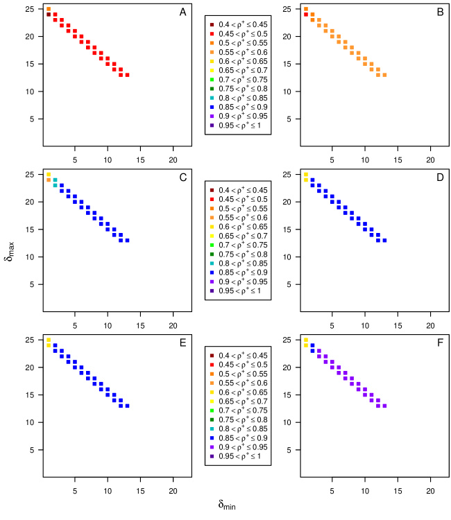
Figure 7: Average value of $\rho_{ij}^{+}$ for type-(iii) graphs as a function of $\delta_{\mathrm{min}}$ and $\delta_{\mathrm{max}}$. Data are given for the first checkpoint (A) through the sixth (F).

For type-(i) graphs (Figure 3), at the first checkpoint most node pairs have $\rho_{ij}^{+}$ values in the interval $(0.4,0.8]$. At the last checkpoint, if we ignore all node pairs for which $\delta_{\mathrm{min}}=1$ for the time being then nearly all node pairs have $\rho_{ij}^{+}$ values in the interval $(0.9,1]$ [the single exception is that of $\delta_{\mathrm{min}}=\delta_{\mathrm{max}}=2$, for which the interval is $(0.85,0.9]$]. The case of type-(ii) graphs (Figure 5), still disregarding all $\delta_{\mathrm{min}}=1$ entries, is closely analogous to that of type-(i) graphs, the differences being that now most node pairs span the larger interval $(0.4,1]$ already at the first checkpoint and that, without exception, at the last checkpoint all node pairs hit the interval $(0.9,1]$. Finally, if we go on focusing on node pairs for which $\delta_{\mathrm{min}}>1$ exclusively, then for type-(iii) graphs (Figure 7) all node pairs have $\rho_{ij}^{+}$ values in the interval $(0.45,0.5]$ at the first checkpoint. At the last checkpoint, on the other hand, this interval becomes $(0.85,0.9]$ if $\delta_{\mathrm{min}}=2$, $(0.9,0.95]$ if $\delta_{\mathrm{min}}>2$.

As Figures 3, 5, and 7 demonstrate, the $\delta_{\mathrm{min}}=1$ case sets itself apart from the others for all graph types at nearly all checkpoints. For example, if we concentrate on the last checkpoint, at which we believe the model’s dynamics to have already settled into some sort of stationary regime [12], then for both type-(i) and type-(ii) graphs it holds that $\rho_{ij}^{+}$ tends to increase from some value in the interval $(0.55,0.6]$ when the girth is $2$ to some value in the interval $(0.9,1]$ when the girth is close to the rough upper bound we set earlier for declaring most node pairs to have been counted [i.e., roughly $18$ for type (i), roughly $12$ for type (ii)]. Naturally, increasing the girth while $\delta_{\mathrm{min}}$ is held fixed at $1$ implies considering node pairs that are progressively more imbalanced, since $\delta_{\mathrm{max}}$ grows with the girth. The case of type-(iii) graphs is different in this respect, as for $\delta_{\mathrm{min}}=1$ all node pairs have $\rho_{ij}^{+}$ values in the interval $(0.6,0.65]$, regardless of which value of $\delta_{\mathrm{max}}$ is in question (either $24$ or $25$). These pairs, however, are of course highly imbalanced as well.

As we mentioned above, a notion that is becoming increasingly central to the study of synchronization in the brain is that of feedback loops, both in a temporal sense (as LFPs and neuronal firing patterns exert influence on one another) and in a spatial sense (as the LFPs of spatially separated areas affect one another). The results we have obtained with our algorithmic model of a cortex lend support to this notion both in the temporal and in the spatial sense.

In the temporal sense we have found ample evidence that our distributed algorithm $A$ is capable of promoting abundant opportunities both for potential to be accumulated in a synchronized way as messages are received at the neurons and for neurons to fire in a synchronized manner. We have found that this holds across all three graph types, from the cortical model first introduced in [12], to an Erdős-Rényi directed graph, to the completely deterministic and tautly shaped structure of a directed circulant graph. In our view, this independence from the graph’s structural characteristics points at an inherent ability of algorithm $A$ at providing some of the elements that help give rise to brain synchronization. Notwithstanding this, our results also do shed some light on the role played by graph structure. As it happens, of the nondeterministic graph types only type-(i) graphs provide the opportunity of long-distance (in the sense of graph distances) synchronization in the two senses we have studied, since distances in type-(ii) graphs are significantly shorter.

In the spatial sense there are two important issues to be highlighted. The first one is that, although by Figure 8 node pairs having higher-than-$18$ girth are rare, they do occur and have yielded high $\rho^{-}$ and $\rho^{+}$ values at all the observational checkpoints. The exact significance this may have in the case of real cortices is unknown, to the best of our knowledge, since spatial feedback loops are known only for very small graph distances [3, 2]. So the fact that they may also occur at significantly larger graph distances remains a tantalizing possibility. The second important issue is the presence of such strong dependence of $\rho^{+}$ on a node pair’s girth when $\delta_{\mathrm{min}}=1$ as we observed. Our results indicate that in this case the synchronization of neuronal spikes is favored on feedback loops involving highly imbalanced pairs of neurons (i.e., node pairs for which $\delta_{\mathrm{max}}\gg 1$). As with the first issue, the significance this may have for real cortices is unknown and merits special attention as further data are obtained.

All our results depend strongly on the measures of synchronization we gave in Equations (3) and (7). They also depend on the model summarized above, but that is now backed up by interesting validating finds [12, 13] and has therefore proven its usefulness as an artificial-life abstraction. It then seems that furthering our study of emerging synchronization properties depends on validating our two measures in a way that ties our causality-based definitions to real data as tightly as possible. We expect to be able to do this as further insight into real cortices becomes available.

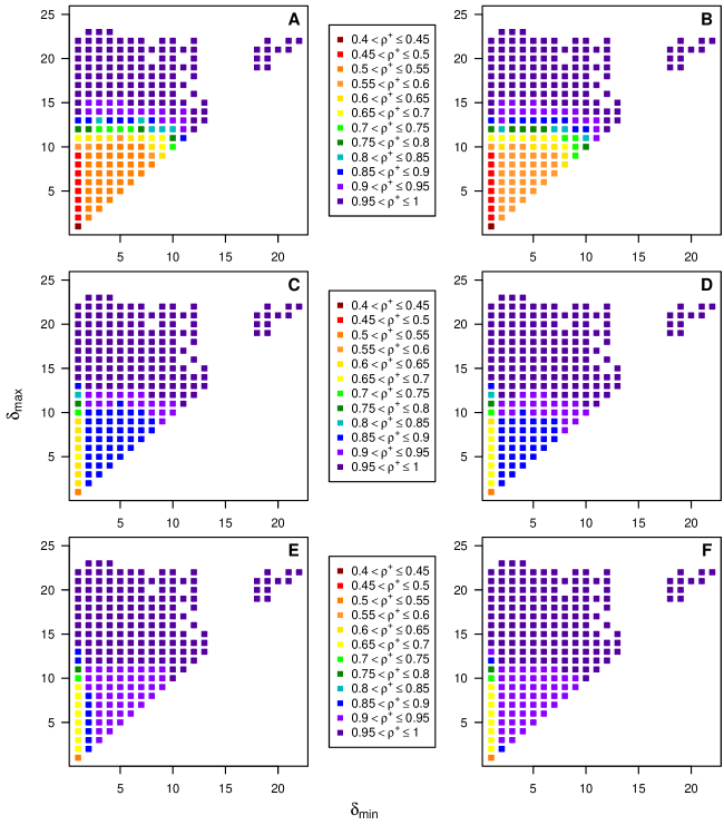
Figure 3: Average value of $\rho_{ij}^{+}$ for type-(i) graphs as a function of $\delta_{\mathrm{min}}$ and $\delta_{\mathrm{max}}$. Data are given for the first checkpoint (A) through the sixth (F).

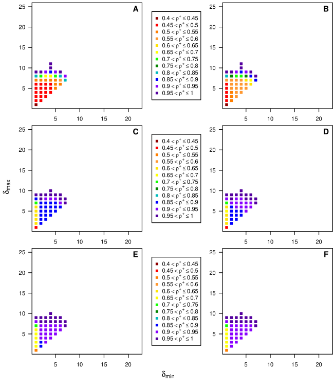
Figure 5: Average value of $\rho_{ij}^{+}$ for type-(ii) graphs as a function of $\delta_{\mathrm{min}}$ and $\delta_{\mathrm{max}}$. Data are given for the first checkpoint (A) through the sixth (F).

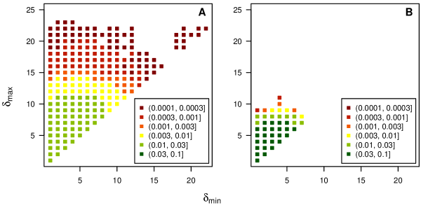
Figure 8: Probability distribution of $\delta_{\mathrm{min}},\delta_{\mathrm{max}}$ pairs for the type-(i) (A) and type-(ii) (B) graphs we used.

References

- 1. Nunez PL, Srinivasan R (2006) Electric Fields of the Brain: The Neurophysics of EEG. New York, NY: Oxford University Press.
- 2. Berens P, Logothetis NK, Tolias AS (2012) Local field potentials, BOLD and spiking activity: Relationships and physiological mechanisms. In: Kriegeskorte N, Kreiman G, editors, Visual Population Codes: Towards a Common Multivariate Framework for Cell Recording and Functional Imaging, Cambridge, MA: The MIT Press. pp. 599–623.
- 3. Fries P (2005) A mechanism for cognitive dynamics: Neuronal communication through neuronal coherence. Trends Cogn Sci 9: 474–480.
- 4. Canolty RT, Ganguly K, Kennerley SW, Cadieu CF, Koepsell K, et al. (2010) Oscillatory phase coupling coordinates anatomically dispersed functional cell assemblies. Proc Natl Acad Sci USA 107: 17356–17361.
- 5. Canolty RT, Knight RT (2010) The functional role of cross-frequency coupling. Trends Cogn Sci 14: 506–515.
- 6. Katzner S, Nauhaus I, Benucci A, Bonin V, Ringach DL, et al. (2009) Local origin of field potentials in visual cortex. Neuron 61: 35–41.
- 7. Huerta R, Bazhenov M, Rabinovich MI (1998) Clusters of synchronization and bistability in lattices of chaotic neurons. Europhys Lett 43: 719–724.
- 8. Lago-Fernández LF, Huerta R, Corbacho F, Sigüenza JA (2000) Fast response and temporal coherent oscillations in small-world networks. Phys Rev Lett 84: 2758–2761.
- 9. Masuda N, Aihara K (2004) Global and local synchrony of coupled neurons in small-world networks. Biol Cybern 90: 302–309.
- 10. Barbour B, Brunel N, Hakim V, Nadal JP (2007) What can we learn from synaptic weight distributions? Trends Neurosci 30: 622–629.
- 11. Song S, Sjöström PJ, Reigl M, Nelson S, Chklovskii DB (2005) Highly nonrandom features of synaptic connectivity in local cortical circuits. PLoS Biol 3: e68.
- 12. Nathan A, Barbosa VC (2010) Network algorithmics and the emergence of the cortical synaptic-weight distribution. Phys Rev E 81: 021916.
- 13. Nathan A, Barbosa VC (2011) Network algorithmics and the emergence of information integration in cortical models. Phys Rev E 84: 011904.
- 14. Balduzzi D, Tononi G (2008) Integrated information in discrete dynamical systems: Motivation and theoretical framework. PLoS Comput Biol 4: e1000091.
- 15. Barbosa VC (1996) An Introduction to Distributed Algorithms. Cambridge, MA: The MIT Press.
- 16. Fisher J, Henzinger TA (2007) Executable cell biology. Nat Biotechnol 25: 1239–1249.
- 17. Fisher J, Harel D, Henzinger TA (2011) Biology as reactivity. Commun ACM 54(10): 72–82.
- 18. Forbes N (2000) Life as it could be: Alife attempts to simulate evolution. IEEE Intell Syst 15(6): 2–7.
- 19. Lindley D (2010) Brains and bytes. Commun ACM 53(9): 13–15.
- 20. Sporns O, Chialvo DR, Kaiser M, Hilgetag CC (2004) Organization, development and function of complex brain networks. Trends Cogn Sci 8: 418–425.
- 21. Sporns O, Tononi G, Kötter R (2005) The human connectome: A structural description of the human brain. PLoS Comput Biol 1: 245–251.
- 22. Achard S, Salvador R, Whitcher B, Suckling J, Bullmore E (2006) A resilient, low-frequency, small-world human brain functional network with highly connected association cortical hubs. J Neurosci 26: 63–72.
- 23. Bassett DS, Bullmore E (2006) Small-world brain networks. Neuroscientist 12: 512–523.
- 24. He Y, Chen ZJ, Evans AC (2007) Small-world anatomical networks in the human brain revealed by cortical thickness from MRI. Cereb Cortex 17: 2407–2419.
- 25. Honey CJ, Kötter R, Breakspear M, Sporns O (2007) Network structure of cerebral cortex shapes functional connectivity on multiple time scales. Proc Natl Acad Sci USA 104: 10240–10245.
- 26. Reijneveld JC, Ponten SC, Berendse HW, Stam CJ (2007) The application of graph theoretical analysis to complex networks in the brain. Clin Neurophysiol 118: 2317–2331.
- 27. Sporns O, Honey CJ, Kötter R (2007) Identification and classification of hubs in brain networks. PLoS ONE 2: e1049.
- 28. Stam CJ, Reijneveld JC (2007) Graph theoretical analysis of complex networks in the brain. Nonlinear Biomed Phys 1: 3.
- 29. Yu S, Huang D, Singer W, Nikolić D (2008) A small world of neuronal synchrony. Cereb Cortex 18: 2891–2901.
- 30. Chialvo DR (2010) Emergent complex neural dynamics. Nat Phys 6: 744–750.
- 31. Modha DS, Ananthanarayanan R, Esser SK, Ndirango A, Sherbondy AJ, et al. (2011) Cognitive computing. Commun ACM 54(8): 62–71.
- 32. Bornholdt S, Schuster HG, editors (2003) Handbook of Graphs and Networks. Weinheim, Germany: Wiley-VCH.
- 33. Newman M, Barabási AL, Watts DJ, editors (2006) The Structure and Dynamics of Networks. Princeton, NJ: Princeton University Press.
- 34. Bollobás B, Kozma R, Miklós D, editors (2009) Handbook of Large-Scale Random Networks. Berlin, Germany: Springer.
- 35. Abeles M (1991) Corticonics: Neural Circuits of the Cerebral Cortex. Cambridge, UK: Cambridge University Press.
- 36. Ananthanarayanan R, Modha DS (2007) Anatomy of a cortical simulator. In: Proc. of the 2007 ACM/IEEE Conf. on Supercomputing. New York, NY: ACM, p. 3.
- 37. Ananthanarayanan R, Esser SK, Simon HD, Modha DS (2009) The cat is out of the bag: Cortical simulations with neurons and synapses. In: Proc. of the Conf. on High Performance Computing Networking, Storage and Analysis. New York, NY: ACM, p. 63.
- 38. Dorogovtsev SN, Mendes JFF, Samukhin AN (2001) Giant strongly connected component of directed networks. Phys Rev E 64: 025101(R).
- 39. Newman MEJ (2005) Power laws, Pareto distributions and Zipf’s law. Contemp Phys 46: 323–351.
- 40. Eguíluz VM, Chialvo DR, Cecchi GA, Baliki M, Apkarian AV (2005) Scale-free brain functional networks. Phys Rev Lett 94: 018102.
- 41. van den Heuvel MP, Stam CJ, Boersma M, Hulshoff Pol HE (2008) Small-world and scale-free organization of voxel-based resting-state functional connectivity in the human brain. Neuroimage 43: 528–539.
- 42. Modha DS, Singh R (2010) Network architecture of the long-distance pathways in the macaque brain. Proc Natl Acad Sci USA 107: 13485–13490.
- 43. Bullmore E, Sporns O (2009) Complex brain networks: Graph theoretical analysis of structural and functional systems. Nat Rev Neurosci 10: 186–198.
- 44. Erdős P, Rényi A (1959) On random graphs. Publ Math (Debrecen) 6: 290–297.
- 45. Freeman WJ, Kozma R, Bollobás B, Riordan O (2009) Scale-free cortical planar networks. In: Bollobás et al. [34], pp. 277–324.
- 46. Sporns O (2011) Networks of the Brain. Cambridge, MA: The MIT Press.
- 47. Amaral LAN, Scala A, Barthélemy M, Stanley HE (2000) Classes of small-world networks. Proc Natl Acad Sci USA 97: 11149–11152.
- 48. Freeman WJ (2007) Scale-free neocortical dynamics. Scholarpedia 2(2): 1357.
- 49. Honey CJ, Sporns O, Cammoun L, Gigandet X, Thiran JP, et al. (2009) Predicting human resting-state functional connectivity from structural connectivity. Proc Natl Acad Sci USA 106: 2035–2040.
- 50. Kaiser M, Hilgetag CC (2004) Modelling the development of cortical systems networks. Neurocomputing 58–60: 297–302.
- 51. Kaiser M, Hilgetag CC (2004) Spatial growth of real-world networks. Phys Rev E 69: 036103.
- 52. Abbott LF, Nelson SB (2000) Synaptic plasticity: Taming the beast. Nat Neurosci 3: 1178–1183.
- 53. Song S, Miller KD, Abbott LF (2000) Competitive Hebbian learning through spike-timing-dependent synaptic plasticity. Nat Neurosci 3: 919–926.
- 54. Bi GQ, Poo MM (1998) Synaptic modifications in cultured hippocampal neurons: Dependence on spike timing, synaptic strength, and postsynaptic cell type. J Neurosci 18: 10464–10472.
- 55. Bi GQ, Poo MM (2001) Synaptic modification by correlated activity: Hebb’s postulate revisited. Annu Rev Neurosci 24: 139–166.
- 56. Kepecs A, van Rossum MCW (2002) Spike-timing-dependent plasticity: Common themes and divergent vistas. Biol Cybern 87: 446–458.
- 57. Henriksen RN (2011) Practical Relativity: From First Principles to the Theory of Gravity. Chichester, UK: Wiley.
- 58. Lamport L (1978) Time, clocks, and the ordering of events in a distributed system. Commun ACM 21: 558–565.
- 59. Innocenti GM, Lehmann P, Houzel JC (1994) Computational structure of visual callosal axons. Eur J Neurosci 6: 918–935.
- 60. Salami M, Itami C, Tsumoto T, Kimura F (2003) Change of conduction velocity by regional myelination yields constant latency irrespective of distance between thalamus and cortex. Proc Natl Acad Sci USA 100: 6174–6179.
- 61. Karp RM (1990) The transitive closure of a random digraph. Random Struct Algor 1: 73–93.
- 62. Lonc Z, Parol K, Wojciechowski JM (2001) On the number of spanning trees in directed circulant graphs. Networks 37: 129–133.
- 63. Bollobás B (1998) Modern Graph Theory. New York, NY: Springer.