Comment on ”Phase transition in a one-dimensional Ising ferromagnet at zero temperature using Glauber dynamics with a synchronous updating mode”

Abstract

Sznajd-Weron in [Phys. Rev. E 82, 031120 (2010)] suggested that the one-dimensional Ising model subject to the zero temperature synchronous Glauber dynamics exhibits a discontinuous phase transition. We show here instead that the phase transition is of a continuous nature and identify critical exponents: $\beta\approx 0$, $\nu\approx 1$, and $z\approx 2$, via a systematic finite-size scaling analysis.

Recently, Sznajd-Weron SW has studied the phase transition in a one-dimensional (1D) Ising ferromagnet at zero temperature using Glauber dynamics with a synchronous update rule. Interestingly, it has been successfully shown that the system exhibits a well-defined phase transition as the parameter $W_{0}$, the spin flipping probability for the null energy difference, is changed. Whereas the absence of the phase transition at a finite temperature in the standard equilibrium Ising chain model is a well-known textbook example, the slow magnetic relaxation in the spin chain systems has become a hot research topic, theoretically and experimentally (see references in SW ).

In the Glauber dynamics of the 1D ferromagnetic spin chain at zero temperature, the energy difference $\Delta E$ is computed for the single-spin flipped configuration, and the spin flip is accepted at the probability SW

$$W(\Delta E)=\left\{\begin{array}[]{ll}1,&\textrm{for}\quad\Delta E<0,\\ W_{0},&\textrm{for}\quad\Delta E=0,\\ 0,&\textrm{for}\quad\Delta E>0.\end{array}\right.$$ (1)

For each site of the system, the above probability is computed and each spin flip at next time step is decided. The synchronous update rule means that all spins in the system are updated at the same time, differently from more commonly used method of the sequential spin update rule. The use of the synchronous update rule enables the system to have the antiferromagnetic ordering, different from the use of the sequential update rule SW . As an order parameter, the density $\rho$ of active bonds which connect different spin values (up and down) is used:

$$\rho=\frac{1}{2L}\sum_{i=1}^{L}(1-\sigma_{i}\sigma_{i+1}),$$ (2)

where $L$ is the number of spins and $\sigma_{i}(=\pm 1)$ is the Ising spin at the $i$th site in the 1D chain with the periodic boundary condition $\sigma_{i+L}=\sigma_{i}$ applied. The density of active bonds is especially useful in the present context, since it can effectively distinguish the ferromagnetic ordering ($\rho=0$) and the antiferromagnetic ordering ($\rho=1$). It should be noted that the system eventually approaches the steady state which is either fully ferromagnetic $\rho_{st}=0$ or fully antiferromagnetic $\rho_{st}=1$, and that the intermediate value inbetween is not possible as the time $t\rightarrow\infty$. Due to the zero temperature nature of the dynamics, the ergodicity is broken and thus the time average and the ensemble average of $\rho_{st}$ are not equivalent to each other. The ensemble average of the order parameter $\langle\rho_{st}\rangle$ in the present context equals the probability of the fully antiferromagnetic stationary state, and thus it can change continuously across the phase transition at $W_{c}$. We emphasize that the continuity of $\langle\rho_{st}\rangle$ does not contradict the discreteness of $\rho_{st}$.

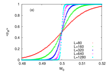
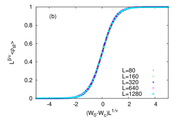
Figure 1: (Color online) (a) Ensemble average $\langle\rho_{st}\rangle$ of the density of active bonds in the steady state versus the spin flipping probability $W_{0}$ for null energy difference, at various system sizes $L=80,160,320,640$, and $1280$. (b) Finite-size scaling of data points in (a) using the scaling form in Eq. (3) with $W_{c}=0.5$, $\beta=0$, and $\nu=1$. The existence of a continuous phase transition is clearly shown. Ensemble averages were performed over $10^{4}$ random initial spin configurations.

Figure 1(a), corresponding to Fig. 4 in SW , displays the ensemble-average of the steady state value of the active bond density $\langle\rho_{st}\rangle$ as a function of the spin flipping probability $W_{0}$ for the null energy difference. We believe that our simulation results and the ones presented in SW are identical and both clearly indicate the existence of the phase transition at $W_{0}=W_{c}(\approx 0.5)$. However, in a sharp contrast to SW where a discontinuous phase transition has been concluded, in this Comment we claim that the system exhibits a continuous phase transition. In order to support our claim of a continuous phase transition, we apply the standard technique of the finite-size scaling goldenfeld of the order parameter $\langle\rho_{st}\rangle$:

$$\langle\rho_{st}\rangle=L^{-\beta/\nu}f\bigl{(}(W_{0}-W_{c})L^{1/\nu}\bigr{)},$$ (3)

where $f(x)$ is a universal scaling function, and $\beta$ and $\nu$ are standard critical exponents, describing the criticality of the order parameter and the coherence length, respectively. In Fig. 1(b), we show the scaling collapse of $\langle\rho_{st}\rangle$ through the use of the scaling form (3). It is very clearly shown that the phase transition at $W_{c}\approx 0.5$ is well captured by $\beta\approx 0.0$ and $\nu\approx 1.0$. The well-defined value of $\nu$ indicates that the coherence length $\xi$ in the system diverges as the critical point is approached, as in a usual continuous phase transition foot .

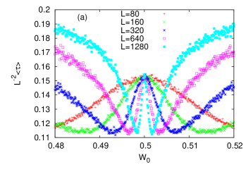
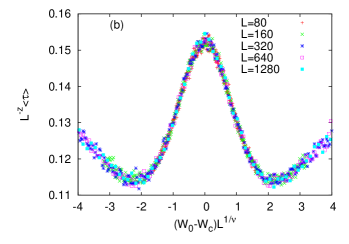
Figure 2: (Color online) (a) The ensemble averaged relaxation time $\langle\tau\rangle$ multiplied by $L^{-2}$ versus the flipping probability $W_{0}$ for various system sizes. (b) Finite-size scaling of relaxation time using the scaling form in Eq. (4) with $W_{c}=0.5$, $\nu=1$, and $z=2$.

The relaxation time $\tau$ for the system to reach the steady state ($\rho=0$ or $1$) from a random initial condition has also been reported in Fig. 5 of SW . We again measure $\tau$ in the same way as in SW and plot it in Fig. 2(a). As was already observed in SW , we also notice that $\langle\tau\rangle$ scales as $L^{2}$ at $W_{c}$. This reminds us that the dynamic critical exponent $z$ goldenfeld describing the divergence of the relaxation time is given by $\tau\sim L^{z}$ exactly at the critical point. Accordingly, the observation of $\tau\sim L^{2}$ strongly indicates $z=2$, and we can write the finite-size scaling form of the relaxation time as

$$\langle\tau\rangle=L^{z}g\bigl{(}(W_{0}-W_{c})L^{1/\nu}\bigr{)},$$ (4)

where $g(x)$ is the scaling function for the relaxation time. The finite-size scaling form (4) satisfies both $\langle\tau\rangle\sim L^{z}$ at $W_{0}=W_{c}$ and $\langle\tau\rangle\sim\xi^{z}$ for $W_{0}\neq W_{c}$ with the prescription $g(x)\sim x^{-\nu z}$ for small $x$ since the correlation length follows $\xi\sim(W_{0}-W_{c})^{-\nu}$. In Fig. 2(b), the scaling collapse of the relaxation time is displayed, which confirms again the existence of the continuous phase transition at $W_{0}=W_{c}(\approx 0.5)$, which is characterized by the coherence length exponent $\nu\approx 1.0$ and the dynamic critical exponent $z\approx 2.0$.

In summary, different from the conclusion in SW , we have clearly shown that the Ising ferromagnet chain at zero temperature with the synchronous update rule exhibits a continuous phase transition at $W_{0}=W_{c}(\approx 0.5)$. Furthermore, through the use of the standard method of the finite-size scaling, we have identified critical exponents $\beta\approx 0.0$, $\nu\approx 1.0$, and $z\approx 2.0$.

This research was supported by Basic Science Research Program through the National Research Foundation of Korea (NRF) funded by the Ministry of Education, Science and Technology (2010-0008758).

References

- (1) K. Sznajd-Weron, Phys. Rev. E 82, 031120 (2010).
- (2) N. Goldenfeld, Lectures on Phase Transitions and the Renormalization Group, (Addison-Wesley, Massachusetts, 1992).
- (3) Although not shown here, we have confirmed that the magnetization and its Binder’s cumulant, the staggered magnetization and its Binder’s cumulant, and also the Binder’s cumulant for , all show good quality of finite-size scalings with the values , , and .