The KCAL VERA 22 GHz calibrator survey

Abstract

We observed at 22 GHz with the VLBI array VERA a sample of 1536 sources with correlated flux densities brighter than 200 mJy at 8 GHz. One half of target sources has been detected. The detection limit was around 200 mJy. We derived the correlated flux densities of 877 detected sources in three ranges of projected baseline lengths. The objective of these observations was to determine the suitability of given sources as phase calibrators for dual-beam and phase-referencing observations at high frequencies. Preliminary results indicate that the number of compact extragalactic sources at 22 GHz brighter than a given correlated flux density level is twice less than at 8 GHz.

1. Introduction

Currently, very long baseline interferometry (VLBI) astrometry is the best tool to measure distances and motions of sources located at kpc scale and hence, to explore the structure of the Milky Way in the Galactic scale. For instance, Japanese VERA project (VLBI Exploration of Radio Astrometry; Honma, Kawaguchi & Sasao (2000)) has been conducting astrometric monitoring of positions of Galactic maser sources with respect to reference compact extragalactic objects, yielding handful measurements of parallaxes and proper motions of maser sources (e.g., see recent PASJ special issue for VERA, such as Honma et al. (2011), Nagayama et al. (2011) and others). The Very Long Baseline Array (VLBA) is actively used for astrometry of Galactic maser sources ((e.g., Reid et al. 2009) and the currently ongoing Bar and Spiral Structure Legacy (BeSSeL) survey) and the European VLBI Network (EVN) conducts astrometric observations of methanol maser sources (e.g., Rygl et al. 2010).

In order to measure parallax and proper motion of a radio source at kpc scales, it is observed in the phase-referencing mode by frequent switching pointing between the target and a calibrator source. This technique significantly reduces phase variations caused by tropospheric fluctuations. To do this effectively, calibrators must be located close to target sources, typically within 1–2° separation. This requires a high density of calibrator sources in the sky, and hence, there is still a strong demand for finding many calibrator sources.

To date, there have been several massive surveys of compact calibrators such as VCS (VLBA Calibrator Surveys), Petrov et al. (2008) and references therein), the LCS (Long Baseline Array Calibrator Survey) for the southern hemisphere (Petrov et al. 2011d), VIPS (VLBA Image and Polarization Survey) (Helmboldt et al. 2007, Petrov & Taylor 2011e), and several ongoing programs: the program of study the Fermi active galaxy nuclea (AGNs) at parsec scales (Kovalev et al. (2011), paper in preparation), the program of observing radio-loud 2MASS (Two Micron All Sky Survey) galaxies (Condon et al. 2011), the program of observing optically bright quasars (Bourda et al. 2008, 2011, Petrov 2011a), and the recent VLBA calibrator search for the BeSSeL survey (Immer et al. 2011).

Together with regular geodetic VLBA observations of 1000 sources Petrov et al. (the RDV program 2009)), by June 2011 positions of 6455 sources at a milliarcsecond level of accuracy were derived from analysis of these massive surveys. The sources turned out compact enough to be detected with VLBI, i.e. they have a core of mas scale. However, these surveys were in most cases conducted in relatively low frequencies such as 2 (S-band), 5 (C-band) or 8 GHz (X-band), at which the telescope performance is the best. On the other hand, recent VLBI maser astrometry is often done at frequencies higher than 10 GHz. For instance, VERA’s main bands are 22 (K-band) and 43 GHz (Q-band) for H₂O and SiO maser sources. Maser astrometry with VLBA is mainly conducted at 12 GHz for CH₃OH masers and 22 GHz for H₂O masers. Therefore, calibrator information at high frequencies (such as K and higher bands) is of great importance for on-going and future astrometric observations. Compact calibrators which are cores of radio bright AGNs have a wide variety of their spectra: for the majority of sources the correlated flux density decreases with the frequency, although some sources may have spectra growing with frequency or peaking within the GHz regime. Hence, the extrapolation of the correlated flux densities from S and X band to 22 or 43 GHz is highly unreliable. For successful phase-reference or dual-beam observations, the correlated flux density should be known with accuracy at least 30% in order to correctly predict the signal-to-noise ratio (SNR). Therefore, it is necessary to conduct a systematic survey of K-band flux densities for the compact sources which were already detected in S and X bands.

We have identified $\sim\!\!2000$ sources previously observed with VLBI with $\delta>-30\arcdeg$ with correlated flux densities $>200$ mJy at X-band at baselines longer than 900 km. Analysis of the dependence of the number of sources $N$ with the correlated flux density exceeding $S$ as a function of $S$ suggests that this sample is complete at the 95% level (Kovalev 2010, private communication). Of these sources, 511 have been previously observed in large K-band surveys: VERA Fringe Search Survey (Petrov et al. 2007), KQ survey (Lanyi et al. 2010), VLBI Galactic plane survey (VGaPS) (Petrov et al. 2011c), in the EVN Galactic plane survey (EGaPS) (Petrov 2011b), and their correlated flux densities at 22 GHz have been measured. The K-band brightness of other objects was not known.

We conducted a dedicated survey of remaining 1536 sources at 22 GHz with VERA in the K-band Calibrator Survey (KCAL) campaign. The goal of these observations was to check their detectability at K-band and to measure the correlated flux densities of detected sources at baselines 1000–2000 km.

The first objective of this campaign was to provide a complete list of calibrators suitable for VERA observations of faint targets. According to our prior observations, the detection limit of the VERA network for 2 minutes of integration time is around 200 mJy, depending on weather conditions. Therefore, the list of sources observed in this and the previous K-band surveys is expected to approach the completeness at the 200 mJy level, provided the spectra of compact cores are flat or falling. According to Massardi et al. (2010) who analyzed simultaneous ATCA spectra at 4.8, 8.4 and 20 GHz, the share of sources with growing spectra that may be missed in our sample does not exceeded 8%.

The second objective of this campaign is to collect information for a population analysis of a large complete sample. In particular, the analysis of the dataset that combines existing and new data will help to answer the question what is the distribution of spectral indexes of the core regions and the source compactness at high frequencies, whether the spectral index at parsec scales is systematically different than the spectral index at kiloparsec scales, and whether the compactness at K-band is systematically different than the compactness at X and S bands.

In this paper we present results of the survey. In section 2 we describe the observations, their design and scheduling. In section 3 we discuss analysis technique. The catalogue of correlated flux densities of detected sources accompanied with analysis of flux density uncertainties is presented in section 4 followed by concluding remarks that are given in section 5.

2. Observations

Observations were carried out using the network of four 20 meter antennas VERA at K-band. The primary task of the array is to perform parallax measurement of maser sources. In order to maximize the throughput of the instrument, observing time for the KCAL experiments was allotted in blocks that fill gaps between parallax measurement observing sessions or during periods of time when one of the antennas was under maintenance.

A monthly observing plan for VERA parallax measurements was usually finalized by at least one week before the beginning of the month. When there were suitable gaps for KCAL experiments and there were enough magnetic tapes in the Mitaka correlation center, we ran calibrator survey experiments during these gaps. The parallax measurement requires participation of each of four stations of VERA in order to achieve required astrometric accuracy. If any station, other than Ogasawara, could not join regular observations because of maintenance or instrumental problems, the KCAL experiments were also scheduled during that time with three stations.

The left circular polarization in the 21.97–22.47 GHz band was received, sampled with 2 bit quantization, and filtered using the VERA digital filter (Iguchi et al. 2005) before being recorded onto magnetic tapes. The digital filter split the data within the 500 MHz band into 16 frequency channels of 16 MHz width each, equally spaced with 16 MHz wide gaps.

2.1. Scheduling

Scheduling software sur_sked selected sources from the pool of candidate objects in a sequence that minimizes slewing time. At a given experiment, each source was observed in one scan of 120 seconds long. Every 30 minutes a scan of a strong source with the brightness distribution map produced from VLBA observations under the KQ observing campaign (Lanyi et al. 2010) was inserted in the schedule. The purpose of including these scans in the schedule was to compare our measurements of the correlated flux densities of sources with known images considered as the ground truth in order to evaluate gain corrections. The target sources which were observed in one scan were returned to the pool for scheduling in the second scan in following experiments.

In total, 36 experiments were scheduled. However, six experiments were canceled for various reasons, in three observing sessions two stations either failed or did not observe; these experiments were excluded from analysis. The dates and durations of the 27 VLBI experiments under the KCAL program over the period 2007–2009 that were used in the analysis are shown in Table 1.

Table 1Dates and durations of experiments. Only those experiments that were used in the final analysis are shown. Station abbreviations: Ir for Iriki, Is for Ishigakijima, Mz for Mizusawa, Og for Ogasawara.

Exp ID	Date	Dur (h)	Network
kcal_01	2007.05.28	5.3	Ir Is Mz Og
kcal_02	2007.05.30	5.8	Ir Is Mz Og
kcal_03	2007.05.31	3.9	Ir Mz Og
kcal_04	2007.08.24	3.8	Ir Is Mz Og
kcal_05	2007.08.24	14.3	Ir Is Mz Og
kcal_06	2007.08.25	6.8	Ir Is Mz Og
kcal_07	2007.11.18	4.8	Ir Is Mz Og
kcal_09	2007.11.23	4.5	Ir Is Mz Og
kcal_10	2007.12.10	5.8	Ir Is Mz Og
kcal_11	2007.12.12	2.6	Ir Mz Og
kcal_12	2007.12.12	2.8	Ir Mz Og
kcal_15	2007.12.19	5.8	Ir Is Mz Og
kcal_16	2007.12.20	3.8	Ir Is Mz Og
kcal_17	2007.12.21	3.8	Ir Is Og
kcal_18	2007.12.22	2.5	Ir Is Og
kcal_19	2007.12.22	3.8	Ir Is Mz Og
kcal_23	2008.02.29	6.8	Ir Is Mz Og
kcal_24	2008.06.03	2.1	Ir Is Mz Og
kcal_25	2008.06.11	5.2	Ir Is Mz Og
kcal_27	2008.10.06	15.8	Ir Is Mz Og
kcal_29	2008.10.12	3.6	Ir Is Mz Og
kcal_30	2008.11.11	2.3	Ir Is Mz Og
kcal_31	2008.11.16	2.1	Ir Is Mz Og
kcal_32	2008.11.14	4.0	Ir Is Mz Og
kcal_33a	2009.03.13	7.9	Ir Is Mz
kcal_33c	2009.03.21	3.9	Ir Is Mz
kcal_33d	2009.03.22	8.8	Ir Is Mz

The scheduling goal of the campaign was to have each target source observed in two experiments, one scan in each observing session. Due to the nature of scheduling in a fill-in mode, it turned out difficult to reach this goal. As it seen from Table 2, 1/3 of the sources were observed in one scan. In total, 1536 target sources were observed for 143 hours. The antennas spent 71% time on target sources. Remaining time was spent for observing the amplitude calibrators and for slewing.

Table 2Statistics of the number of scans per observed source. The first columns shows the number of scans, the second table shows the number of target sources which had that number of scans. The last column shows the share of sources from the target list which had that number of scans.

# scans	# obs	Share
1	530	35%
2	633	41%
3	267	17%
4	102	5%
5	4	0.2%

3. Data analysis

3.1. Fringe fitting

The data were correlated on the Mitaka FX correlator (Chikada et al. 1991). Correlation output was written in the FITS-IDI format. Consecutive analysis was performed with computer program $\cal PIMA$ . The procedure of data analysis is described in detail in Petrov et al. (2011c). Here only a brief outline is given. After applying correction of fringe amplitude for digitization, the spectrum of the cross-correlation function was presented as a two-dimensional array with the first dimension running over frequency channels and the second dimension running over time. The two-dimensional Fourier-transform of the spectrum over frequency and time cast the spectrum of the cross-correlation function into the domain of group delay and phase delay rate. A set of estimates of delays, phase delay rates and fringe amplitude for a given scan at a given baseline is thereafter called observation. In the presence of the signal in the data, the Fourier-transform of the cross-spectrum exhibits a sequence of peaks. The amplitude of the major peak is proportional to the fringe amplitude of the signal. The fringe fitting process locates the peaks and determines the group delay, delay rate and fringe amplitude that correspond to the main maximum of the Fourier-transform of the cross-correlation spectrum.

In order to determine the detection threshold, first we have to measure the noise level. To do this, we computed the ratios of fringe amplitudes to mean amplitudes of the Fourier-transform of the cross-correlation spectrum. That mean amplitude was computed by averaging 32768 randomly selected samples of the cross-spectrum Fourier-transform after iterative excluding the amplitudes that are greater than 3.5 times of the variance of amplitudes in the sample, in order to be sure that no samples with the signal were selected by accident. This procedure ensures that the mean amplitude of the noise is determined with an accuracy no worse than 1%.

Even in the absence of the signal, the fringe fitting procedure will find a peak, but the amplitude of this peak will not be related to the fringe amplitude. The distribution of the achieved SNRs consists of the contribution of the population of observations with signal detected and the population of observations without signal. The SNR probability density in the absence of signal is described (for instance (Petrov et al. 2011c)):

$$p(s)=\frac{\displaystyle 2}{\displaystyle\pi}\frac{\displaystyle n_{\rm eff}}{\displaystyle\sigma_{\rm eff}}\,s\,e^{-\frac{s^{2}}{\pi}}\left(1-e^{-\frac{s^{2}}{\pi}}\right)^{n_{\rm eff}-1},$$ (1)

where $n_{\rm eff}$ is the effective number of independent samples and $\sigma_{\rm eff}$ is the effective noise variance.

In order to determine $n_{\rm eff}$ and $\sigma_{\rm eff}$, we computed the histogram of the achieved SNR in the KCAL experiments in the range of [3.8, 6.5] (see Figure 1) and fitted it with the theoretical curve $p(s)$ of the fringe amplitude distribution in the absence of the signal. The left tail of the SNR histogram is dominated by non-detected sources. The right tail is dominated by detected sources. The breakdown occurs with SNR in a range of [5, 6.5]. There is some fraction of detected sources with the SNR within the range of [5, 6.5], and they potentially may cause a bias in our estimates of $n_{\rm eff}$ and $\sigma_{\rm eff}$. We varied the range of SNRs used for fitting and found that the estimates are stable at a level of $10^{-3}$, i.e. the bias is negligible.

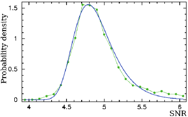
Figure 1.— The left tail of the empirical distribution of the achieved SNR from results of fringe fitting VERA data (filled circles) and the fitted curve (thin line) of the theoretical distribution for the case of no signal.

After determining $n_{\rm eff}$ and $\sigma_{\rm eff}$, we can find the probability that an observation with a given SNR belongs to the population of observations without a signal, i.e. the probability of false detection, by integrating expression 1 over $s$, which can be easily done analytically. Specifically, we found that the probability of false detection is less than 0.001 when the $\rm SNR\ >6.03$. We considered a source as detected if the SNR in at least two observations at different baselines of the same scan was above the detection limit 6.03. In the absence of the signal, the probability of finding two peaks exceeding the threshold limit in data of different observations is in the range of $10^{-3}$ to $10^{-6}$ depending whether the errors are completely correlated or completely uncorrelated. In practical terms, this means that our catalogue may have no more than one or two falsely detected objects.

3.2. Amplitude calibration

System temperatures including atmospheric attenuation were measured with the chopper-wheel method (Ulich & Haas 1976). At the beginning of each scan, a microwave absorber at ambient temperature was inserted just in front of the feed horn, and the received total power was measured with a power meter. Using the measured total power for the blank sky and the absorber, the temperature scale automatically corrected for the atmospheric attenuation was determined. We estimate the uncertainty in the temperature scale around 10%, mainly due to the assumption that the ambient temperature is the same as the air temperature.

The initial amplitude calibration was made by scaling fringe amplitudes, determined with the fringe fitting process, by the measured system temperature and dividing them by the antenna gain. Then, the antenna gains were adjusted by comparing the calibrated fringe amplitudes of the observed calibrator sources with the correlated flux densities predicted on the basis of their K-band brightness distributions:

$$\begin{array}[]{lcl}F_{corr}&=&\left|\displaystyle\sum_{j}c_{j}(x,y)\,e^{\frac{2\pi i\,f}{c}\,(u\,x+v\,y)}\right|,\\ \end{array}$$ (3)

where $c_{i}$ is the correlated flux density of the $j$th CLEAN component with coordinates $x$ and $y$ with respect to the center of the image; $u$ and $v$ are the projections of the baseline vectors onto the tangential plane of the source.

Then we built a system of equations for all observations of calibrators:

$$\mbox{$F_{\rm corr}$}=\sqrt{g_{i}\,g_{j}}\mbox{$A_{\rm corr}$}$$ (4)

that relates the calibrated amplitude $A_{\rm corr}$, gain corrections $g$ for stations $i$ and $j$ of a baseline, and the predicted correlated flux of the amplitude calibrator. After taking logarithms from left and right hand sides, we solved for average gains corrections for all stations using the least squares (LSQ) technique. Then an iterative procedure of outliers elimination was performed. At each step of iterations, we computed the rms of the ratio of observed and predicted correlated flux densities. We searched for the observation with the maximum by module logarithm of this ratio. If the ratio for that observation exceeded $3.5\sigma$ rms, we excluded the observation from the system of equations and ran a new LSQ solution. The process was repeated till no observations with the maximum by module logarithm exceeding $3.5\sigma$ rms was found.

The number of calibrators in each individual experiment varied. On average, 9 calibrators were used for gain correction adjustment in each experiment. If the model brightness distributions were perfect, and gain corrections were stable over an experiment, calibration errors would have been below the noise level. Several factors can degrade the quality of calibration using this method. First, the images of calibrator sources were produced using observations at different sampling of spatial frequencies than the analyzed observations. Computation of the predicted correlated flux densities is equivalent to an interpolation of visibilities measured in KQ and VGaPS VLBA campaigns to $u$ and $v$ baseline projections in the KCAL experiments. Errors of this interpolation may be significant, except for sources with very simple structure. Second, both source structure and the peak brightness evolve with time. Since the time difference in epochs between KQ, VGaPS and KCAL experiments is 2–6 years, the changes in source brightness distribution may be significant. The sampling bias and the source variability are expected to cause only random errors in gain, but not a systematic bias. Some calibrator sources may become brighter, some dimmer, but the average flux density of the ensemble should be rather stable. Third, we assumed that gain corrections are constant over time of an individual experiment since we do not have enough information for modeling their time variability.

4. The correlator flux density catalogue

Since the data are too sparse to produce meaningful images, we computed average correlated flux densities for detected sources in three ranges of projected baseline lengths: 0–70 megawavelengths, 70–100 megawavelengths, and 100–250 megawavelengths, which corresponds to lengths 0–955 km, 955–1365 km, and longer that 1365 km respectively. The corresponding resolutions are $>3$ mas for the first range, 2–3 mas for the second range, and $<2$ mas for the third range. The amplitudes were calibrated for gain corrections using the method described in the previous section. This simplified method of correlated flux density evaluation is an alternative to a rigorous imaging procedure in the case when there are too few measurements.

The catalogue of correlated flux densities of 877 observed sources, including 750 targets and 127 calibrators, is presented in table 3. Objects with at least two detections are put in the catalogue. Columns 1 and 2 show IAU and IVS source names. Column 3 shows the source status: C stands for an amplitude calibrator, blank stands for a target object. Column 4 shows the number of experiments in which a source was detected and column 5 shows the total number of detections. Columns 6, 7, and 8 present the estimates of the average correlated flux density in three ranges of the projected baseline lengths. Columns 9, 10, and 11 show the estimates of correlated flux density uncertainty: $\sigma(\mbox{$F_{\rm corr}$})=\mbox{$A_{\rm corr}$}\cdot\sqrt{0.2^{2}+\frac{2}{\pi}\frac{1}{\rm SNR^{2}}}$. Columns 12 and 13 show right ascensions and declinations. Value $-1.000$ in columns 6–11 indicates a lack of results for these baseline projections.

Table 3The first 12 rows of the catalogue of correlated flux densities of 877 sources that have at least two detections in VERA KCAL observing campaign. The table columns are explained in the text. The full table is available in the electronic attachment.

Source names			Statistics		Corr. flux density			Errors of $F_{\rm corr}$			Source coordinates
(1)	(2)	(3)	(4)	(5)	(6)	(7)	(8) aaa	(9)	(10)	(11) aaa	(12)	(13)
IAU name	IVS name	flag	#Exp	#Det	$F_{<70}$	$F_{70-100}$	$F_{>100}$	$E_{<70}$	$E_{70-100}$	$E_{>100}$	Right ascen	Declination
					Jy	Jy	Jy aaa	Jy	Jy	Jy aaa	h 0m 0s	00$\arcdeg\phantom{0}\phantom{0}{}^{\prime}\phantom{0}\phantom{0}{}^{\prime\prime}$
J0001$+$1914	2358$+$189		1	4	0.221	0.322	0.216	0.055	0.070	0.051	00 01 08.62	$+$19 14 33.8
J0005$+$3820	0003$+$380		2	8	-1.000	0.608	0.526	-1.000	0.136	0.116	00 05 57.17	$+$38 20 15.1
J0006$-$0623	0003$-$066		2	9	1.027	1.120	1.212	0.104	0.205	0.176	00 06 13.89	$-$06 23 35.3
J0008$+$6837	0005$+$683		1	2	-1.000	0.353	-1.000	-1.000	0.080	-1.000	00 08 33.47	$+$68 37 22.0
J0010$+$1058	IIIZ$W$2	C	2	6	-1.000	1.193	1.442	-1.000	0.239	0.289	00 10 31.00	$+$10 58 29.5
J0010$+$1724	0007$+$171		1	2	-1.000	0.340	0.266	-1.000	0.078	0.060	00 10 33.99	$+$17 24 18.7
J0010$-$2157	0008$-$222		1	2	-1.000	0.236	-1.000	-1.000	0.052	-1.000	00 10 53.64	$-$21 57 04.2
J0011$+$7045	0008$+$704		2	8	0.440	0.405	0.542	0.043	0.088	0.064	00 11 31.90	$+$70 45 31.6
J0012$-$3954	0010$-$401		1	3	0.505	0.494	-1.000	0.120	0.103	-1.000	00 12 59.90	$-$39 54 26.0
J0013$+$4051	0010$+$405		2	7	0.531	0.534	0.492	0.065	0.119	0.115	00 13 31.13	$+$40 51 37.1
J0013$-$0423	0011$-$046		2	7	0.552	0.406	0.445	0.071	0.094	0.101	00 13 54.13	$-$04 23 52.2
J0017$+$5312	0015$+$529		1	2	-1.000	0.270	-1.000	-1.000	0.067	-1.000	00 17 51.75	$+$53 12 19.1

Note. — Table 3 is presented in its entirety in the electronic edition of the Astronomical Journal. A portion is shown here for guidance regarding its form and contents.

Of 1536 observed sources, including both targets and calibrators, 407 were not detected at all and 252 were detected only in one observation. The detections from the latter group were considered unreliable and were not included in the catalogue.

4.1. Error analysis

Errors in correlated flux density estimates are due to 1) the thermal noise in estimates of fringe amplitude; 2) the uncertainties in system temperature measurements; 3) the uncertainties in antenna gain measurement; 4) the sampling bias in predicted correlated flux densities of calibrators; 5) the variability of calibrator sources.

The uncertainty due to the thermal noise can be easily evaluated as $\sqrt{2/\pi<\!\!a_{n}\!\!>/a}$, where $<\!\!a_{n}\!\!>$ is the average amplitude of the noise computed by the fringe fitting procedure, and $a$ is the fringe amplitude. As we already mentioned, the uncertainty in system temperature measurement is around 10%. The aperture efficiency of VERA antenna is measured every year and known within 10% accuracy (see VERA status report). We assume these two uncertainties uncorrelated, and therefore, these two factors would introduce an uncertainty of the a priori gain calibration at $\sim\!14\%$ level.

Since on average, nine amplitude calibrators were used for gain adjustments, this redundancy can be exploited for evaluation the gain correction uncertainties. We computed the average and the root mean square (rms) of the residual mismatches between observed correlated flux densities of calibrators after applying gain corrections $A^{p}_{\rm corr}$ from the LSQ fit and the predicted correlated flux densities from the brightness distributions:

$$\begin{array}[]{lcl}\mbox{\rm Avr}&=&\left(\displaystyle\prod\limits_{i}\frac{\displaystyle\mbox{$F_{\rm corr}$}_{,i}\sqrt{g_{1}g_{2}}}{\displaystyle\mbox{$A^{p}_{\rm corr}$}_{,i}}\right)^{1/n}\vspace{1ex}\\ \mbox{\rm Rms}&=&\sqrt{\frac{\displaystyle\displaystyle\sum_{i}\left(\frac{\displaystyle\mbox{$F_{\rm corr}$}_{,i}\sqrt{g_{1}g_{2}}}{\displaystyle\mbox{$A^{p}_{\rm corr}$}_{,i}}-1\right)^{2}}{\displaystyle n}}.\end{array}$$ (7)

We found Avr = 0.994 and Rms = 0.21. The first statistics describes the systematic bias and the second statistics is the measure of the contribution of uncertainties in gain adjustments on the uncertainty of our estimate of the correlated flux density.

In order to evaluate the representativeness of this statistics, we computed the median correlated flux densities in three ranges of projected baseline lengths of two experiments of the 24 GHz VLBA VGaPS campaign using two methods: 1) rigorous self-calibration imaging and 2) the same simplified method used for processing KCAL experiments. In order to closely mimic analysis of the KCAL experiments, we used for our tests the brightness distributions from the KQ campaign made at epochs at least one year prior to observations. We got Avr = 0.996 and Rms = 0.24. Then we computed the rms of the scatter of the ratios of the correlated flux density $F^{s}_{\rm corr}$ determined by the simplified method to the flux density $F^{r}_{\rm corr}$ determined by the rigorous method: rms = $\sqrt{\sum_{i}(\mbox{$F^{s}_{\rm corr}$}_{,i}/\mbox{$F^{r}_{\rm corr}$}_{,i}-1)^{2}}$. We found the rms equal to 0.15. Considering the brightness distributions from the self-calibration analysis procedure as the ground truth, we conclude that the accuracy of the median correlated flux density obtained by the simplified method is at a level of 15% for the VGaPS campaign. Thus, the Rms statistics give us rather an upper limit of gain errors.

Another way to evaluate the average uncertainty of correlated flux densities is to compute the rms of the scatter of ratios of the correlated flux densities of a given source with respect to the mean value for all the KCAL sources which have three or more observations. We got the value of the rms 0.20, which is close to the Rms statistics. Therefore, we conclude that the average uncertainty of calibration error is 20%. Since the uncertainty in fringe amplitude caused by the thermal noise and calibration errors are independent, we compute the multiplicative uncertainty of reported correlated flux density as a sum of these two contributions in quadrature: 0.2 and $\sqrt{\frac{2}{\pi}}\frac{1}{\rm SNR}$.

5. Concluding remarks

We observed with VERA at 22 GHz a subset of the complete sample of continuum compact extragalactic sources with correlated flux densities $>200$ mJy at X-band at declinations $>-30\arcdeg$. The subset excluded the sources previously detected at K-band at large VLBA and VERA surveys. Of 1536 target sources, approximately one half has been detected. The errors of the correlated flux densities are a level of 20%.

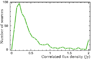
Figure 2.— The distribution of the correlated flux densities at baseline projection lengths longer than 100 megawavelengths. The last bin of the histogram has all the sources with correlated flux density $>2$ Jy.

Figure 2 shows the distribution of the KCAL correlated flux densities. Assuming that the parent population of sources is uniform in the range of flux densities 1–1000 mJy, we explain the sudden drop in the number of sources with correlated flux densities below 200 mJy as an indication of under-representation of sources weaker than that limit in the catalogue because they are not reliably detected with VERA. Thus, the KCAL is incomplete at flux densities below 200 mJy. This result is in agreement with our analysis of previous VERA observations (Petrov et al. 2007) where we estimated the probability of detection of a source with the correlated flux density 200 mJy at a level of 70%.

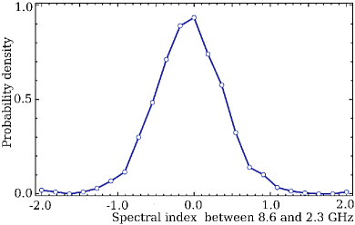
Figure 3.— The distribution of the spectral indices $\alpha$ ($F(\nu)\sim\,v^{\alpha}$) of 1536 sources from the input catalogue. The spectral index was computed from median correlated flux densities at 8.6 and 2.3 GHz at baseline projected lengths shorter than 900 km.

The detection limit of VERA at 22 GHz, 200 mJy, corresponded the lowest correlated flux density of the input source list, 200 mJy, at 8 GHz. The majority of the sources from the input list were previously observed at VLBI at both 8.6 and 2.3 GHz. The distribution of spectral indices ($F(\nu)\sim\,v^{\alpha}$) of the compact component of these sources shows a peak near spectral index 0 (see Figure 3). Among 1536 sources from the input list, 48% had spectral index greater then zero, and therefore, their extrapolated flux density at 22 GHz was greater than 200 mJy, the average detection limit of the KCAL survey. Although a measured correlated flux density at 22 GHz for an individual source may be less of greater than the flux density extrapolated from 8.6/2.3 GHz, if to consider the entire population as a whole, the measured flux density at 22 GHz turned out on average very close to the extrapolated one.

Results of the KCAL survey augmented with results of prior K-band surveys form the list of objects with known correlated flux densities. By June 2011, this list contained 1161 objects. Among these sources, 766 objects have correlated flux densities greater than 200 mJy at baselines shorter than 70 M$\lambda$ and 608 objects are brighter than 200 mJy at baselines longer than 100 M$\lambda$. These sources are considered as a pool of calibrators for VERA in 2011. After completion of a planned sensitivity upgrade, even weaker sources can be used for calibrators.

We reserve a rigorous population analysis to a future publication. Preliminary results indicate that the number of compact extragalactic sources at K-band brighter than a given correlated flux density level is twice less than at the X-band.

We would like to thank Alan Fey for making publicly available not only contour plots of images from the KQ survey, but brightness distribution and calibrated flux densities in the FITS-format. The availability of this information was crucial for our project.

References

- Bourda et al. (2008) Bourda, G., Charlot, P., & Le Campion, J.-F. 2008, A&A, 490, 403
- Bourda et al. (2011) Bourda, G., Collioud, A., Charlot, P., Porcas, R. W., & Garrington, S. T. 2011, A&A, 526, A102
- Condon et al. (2011) J. Condon, J. Darling, Y. Y. Kovalev, L. Petrov, 2011, preprint, http://arxiv.org/abs/1110.6252
- Chikada et al. (1991) Chikada, Y., et al. 1991, in Frontiers of VLBI, ed. H. Hirabayashi, M. Inoue, & H. Kobayashi, Tokyo: Universal Academy Press, 79
- Helmboldt et al. (2007) Helmboldt, J. F., Taylor, G. B., Tremblay, S., Fassnacht, C. D., Walker, R. C., Myers, S. T., Sjouwerman, L. O., Pearson, T. J., Readhead, A. C. S., Weintraub, L., Gehrels, N., Romani, R. W., Healey, S., Michelson, P. F., Blandford, R. D., Cotter, G. 2007, ApJ, 658, 203
- Honma, Kawaguchi & Sasao (2000) Honma, M., Kawaguchi, N., Sasao, T. 2000, in Proc. SPIE, 4015, Radio Telescope, ed. H. R. Buthcer, 624
- Honma et al. (2011) Honma, M., Hirota, T., Kan-Ya, Y., Kawaguchi, N., Kobayashi, H., Kurayama, T., Sato, K. 2011, PASJ, 63, 17
- Iguchi et al. (2005) Iguchi, S., Kurayama, T., Kawaguchi, N., and Kawakami, K. 2005, PASJ, 57, 259
- Immer et al. (2011) Immer, K. et al., 2011, ApJS, 194, 25
- Lanyi et al. (2010) Lanyi G. E. et al. 2010, AJ, 139, 1695
- Massardi et al. (2010) Massardi M. et al., 2011, MNRAS, 412, 318
- Nagayama et al. (2011) Nagayama, T., Omodaka, T., Nakagawa, A., Handa, T., Honma, M., Kobayashi, H., Kawaguchi, N., Miyaji, T. 2011, PASJ, 63, 23
- Petrov et al. (2007) Petrov L., Hirota T., Honma M., Shibata S. M., Jike T., Kobayashi H. 2007, AJ, 133, 2487
- Petrov et al. (2008) Petrov L., Kovalev Y. Y., Fomalont E., Gordon D., 2008, AJ, 136, 580
- Petrov et al. (2009) Petrov L., Gordon D., Gipson J., MacMillan D., Ma C., Fomalont E., Walker R. C., Carabajal C., 2009, Jour. Geodesy, 83(9), 859
- Petrov (2011a) Petrov L. 2011a, AJ, 142, 105
-
Petrov (2011b)
Petrov L., 2011b, MNRAS, in press
(http://arxiv.org/abs/1106.4883) - Petrov et al. (2011c) Petrov L., Kovalev Y. Y., Fomalont E., Gordon D., 2011c, AJ, 142, 35
- Petrov et al. (2011d) Petrov L., Phillips, C., Bertarini, A., Murphy, T., Sadler, E. M., 2011d, MNRAS, 414(3), 2528
- Petrov & Taylor (2011e) Petrov, L., Taylor, G. B., AJ, 2011e, 142, 89
- Reid et al. (2009) Reid, M. J., Menten, K. M., Zheng, X. W., Brunthaler, A., Moscadelli, L., Xu, Y., Zhang, B., Sato, M., Honma, M., Hirota, T., Hachisuka, K., Choi, Y. K., Moellenbrock, G. A., Bartkiewicz, A. 2009, ApJ, 700, 137
- Rygl et al. (2010) Rygl, K. L. J., Brunthaler, A., Reid, M. J., Menten, K. M., van Langevelde, H. J., & Xu, Y. 2010, A&A, 511, A2
- Ulich & Haas (1976) Ulich, B. L., & Haas, R. W. 1976, ApJS, 30, 247