Surface tension of multi-phase flow with multiple junctions governed by the variational principle

Abstract

We explore a computational model of an incompressible fluid with a multi-phase field in three-dimensional Euclidean space. By investigating an incompressible fluid with a two-phase field geometrically, we reformulate the expression of the surface tension for the two-phase field found by Lafaurie, Nardone, Scardovelli, Zaleski and Zanetti (J. Comp. Phys. 113 (1994) pp.134-147) as a variational problem related to an infinite dimensional Lie group, the volume-preserving diffeomorphism. The variational principle to the action integral with the surface energy reproduces their Euler equation of the two-phase field with the surface tension. Since the surface energy of multiple interfaces even with singularities is not difficult to be evaluated in general and the variational formulation works for every action integral, the new formulation enables us to extend their expression to that of a multi-phase ($N$-phase, $N\geq 2$) flow and to obtain a novel Euler equation with the surface tension of the multi-phase field. The obtained Euler equation governs the equation of motion of the multi-phase field with different surface tension coefficients without any difficulties for the singularities at multiple junctions. In other words, we unify the theory of multi-phase fields which express low dimensional interface geometry and the theory of the incompressible fluid dynamics on the infinite dimensional geometry as a variational problem. We apply the equation to the contact angle problems at triple junctions. We computed the fluid dynamics for a two-phase field with a wall numerically and show the numerical computational results that for given surface tension coefficients, the contact angles are generated by the surface tension as results of balances of the kinematic energy and the surface energy. Keywords: multi-phase flowsurface tensionmultiple junctionvolume-preserving diffeomorphism

37K65 58E12 76T30 76B45

1 Introduction

Recently, since the developments of both hardware and software in computer science enable us to simulate complex physical processes numerically, such computer simulations become more important from industrial viewpoints. Especially the computation of the incompressible multi-phase fluid dynamics has crucial roles in order to evaluate the behavior of several devices and materials in a micro-region, e.g., ink-jet printers, solved toners and so on. In the evaluation, it is strongly required that the fluid interfaces with multiple junctions are stably and naturally computed from these practical reasons.

In this article, in order to handle the fluid interfaces with multiple junctions in a three dimensional micro-region, we investigate a surface tension of an incompressible multi-phase flow with multiple junctions as a numerical computational method under the assumption that the Reynolds number is not so large. In the investigation, we encounter many interesting mathematical objects and results, which are associated with low dimensional interface geometry having singularities, and with the infinite dimensional geometry of incompressible fluid dynamics. Further since even in a macroscopic theory, we introduce artificial intermediate regions in the material interfaces among different fluids or among a solid and fluids, the regions give a resolution of the singularities in the interfaces to provide extended Euler equations naturally. Thus even though we consider the multi-phase fluid model as a computational model, we believe that it must be connected with mathematical nature of real fluid phenomena as their description. We will mention the background, the motivation and the strategy of this study more precisely as follows.

For a couple of decades, in order to represent the physical process with the interfaces of the multi-phase fluids, the computational schemes have been studied well. These schemes are mainly classified into two types. The first type is based on the level-set method [42] discovered by H-K. Zhao, T. Chan, B. Merriman, S. Osher and L. Wang [46, 45]. The second one is based on the phase-field theory, which was found by J. U. Brakbill, D. B. Kothe and C. Zemach [11], and B. Lafaurie, C. Nardone, R. Scardovelli, S. Zaleski, and G. Zanetti [31]. The authors in Reference [31] called the scheme SURFER. Following them, there are many studies on the SURFER scheme, e.g., [7, 12, 24, references therein].

The level-set method is a computational method in which we describe a (hyper-)surface in terms of zeros of the level-set function, i.e., a real function whose value is a signed distance from the surface, such as $q(x)$ in Section 2.1. Using the scheme based upon the level-set method in the three dimensional Euclidean space, we can deal well with topology changes, geometrical objects with singularities, e.g., cusps, the multiple junctions of materials, and so on. However in the computation, we need to deal with the constraint conditions even for two-phase fluids [46, 45]. A dynamical problem with constraint conditions is basically complicate and sometimes gives difficulties to find its solution since the constraint conditions sometimes generate an ill-posed problem in the optimization. In the numerical computation for incompressible fluid, we must check the consistency between the incompressible condition and the constraint condition. The check generally requires a complicate implementation of the algorithm, and increases computational cost. Its failure sometimes makes the computation unstable, especially when we add some other physical conditions. Since instability disturbs the evaluation of a complex system as a model of a real device, it must be avoided.

On the other hand, using the SURFER scheme [31], we can easily compute effects of the surface tension of a two-phase fluid in the Navier-Stokes equation. The phase field model is the model that we represent materials in terms of supports of smooth functions which roughly correspond to the partition of unity in pure mathematics [27, I p.272] as will be mentioned in Sections 4 and 5. We call these functions “color functions” or “phase fields”. The phase fields have artificial intermediate regions which represent their interfaces approximately. In the SURFER scheme [31], the surface tension is given as a kind of stress force, or volume force due to the intermediate region. Hence the scheme makes the numerical computations of the surface tension stable. However it is not known how to consider a multi-phase ($N$-phase, $N\geq 2$) flow in their scheme. In Reference [11], the authors propose a method as an extension of the SURFER scheme [31] to the contact angle problem by imposing a constraint to fix its angle. In this article, we will generalize the SURFER scheme to multi-phase flow without any constraints.

Nature must not impose any constraints even at such a triple junction, which is governed by a physical principle. If it is a Hamiltonian system, its determination must obey the minimal principle or the variational principle. We wish to find a theoretical framework in which we can consistently handle the incompressible flows with interfaces including the surface tensions and the multiple junctions without any constraints. As the multiple junctions should be treated as singularities in a mathematical framework which are very difficult to be handled in general, it is hard to extend mathematical approaches for fluid interface problems without a multiple junction [8, 40] to a theory for the problem with multiple junctions. Our purpose of this article is to find such a theoretical framework which enables us to solve the fluid interface problems with multiple junctions numerically as an extension of the SURFER scheme.

For the purpose, we employ the phase field model. The thickness of the actual intermediate region in the interface between a solid and a fluid or between two fluids is of atomic order and is basically negligible in the macroscopic theory. However the difference between zero and “the limit to zero” sometimes brings a crucial difference in physics and mathematics; for example, in the Sato hyperfunction theory, the delta function is regarded as a function in the boundary of the holomorphic functions [26, 29], i.e., $\displaystyle{\delta(x)=\lim_{\epsilon\to 0}\frac{1}{2\pi{\rm{i}}}\left(\frac{1}{x-{\rm{i}}\epsilon}-\frac{1}{x+{\rm{i}}\epsilon}\right)}$ $\displaystyle{\equiv\lim_{\epsilon\to 0}\frac{1}{\pi}\frac{\epsilon}{x^{2}+\epsilon^{2}}}$. As mentioned above, the phase field model has the artificial intermediate region which is controlled by a small parameter $\epsilon$ and appears explicitly even as a macroscopic theory. We regard that it represents the effects coming from the actual intermediate region of materials. Namely, we regard that the stress force expression in the SURFER scheme is caused by the artificial intermediate region of the phase-fields and it represents well the surface effect coming from that of real materials.

In order to extend the stress force expression of the two-phase flow to that of the multi-phase ($N$-phase, $N\geq 2$) flow, we will first reformulate the SURFER scheme in the framework of the variational theory. In Reference [24], a similar attempt was reported but unfortunately there were not precise derivations. Our investigations in Section 4 show that the surface tension expression of the SURFER scheme is derived as a momentum conservation in Noether’s theorem [10, 23] and its derivation requires a generalization of the Laplace equation [30] as the Euler-Lagrange equation [5, 10], which is not trivial even for a static case.

In order to deal with this problem in a dynamics case consistently, we should also consider the Euler equation in the framework of the variational principle. It is well-known that the incompressible fluid dynamics is geometrically interpreted as a variational problem of an infinite dimensional Lie group, related to diffeomorphism, due to V. I. Arnold [1, 4], D. Ebin and J. Marsden [18], H. Omori [38] and so on. Following them, there are so many related works [6, 9, 25, 37, 41, 43, 44, 49].

On the reformulation of the SURFER scheme [31] for the dynamical case, we introduce an action integral including the kinematic energy of the incompressible fluid and the surface energy. The variational method reproduces the governing equation in the SURFER scheme.

After then, we extend the surface energy to that of multi-phase fields and add the energy term to the action integral. The variational principle of the action integral leads us to a novel expression of the surface tension and the extended Euler equation which we require. Using the extended Euler equation, we can deal with the surface tensions of the multi-phase flows, the multiple junctions of the of phase fields including singularities, the topology changes and so on. We can also compute a wall effect naturally and a contact angle problem. The computation of the governing equation is freed from any constraints, except the incompressible condition.

In other words, in this article, we completely unify the theory of the multi-phase ($N$-phase, $N\geq 2$) field and the theory of the incompressible fluid dynamics of Euler equation as an infinite dimensional geometrical problem.

Contents are as follows: Section 2 is devoted to the preliminaries of the theory of surfaces in our Euclidean space from a low-dimensional differential geometrical viewpoint [34, 20, 19] and Noether’s theorem in the classical field theory [5, 10, 23]. Section 3 reviews the derivation of the Euler equation to the incompressible fluid dynamics following the variational method for an infinite-dimensional Lie algebra based upon Reference [18]. In Section 4, we reformulate the SURFER scheme [31]. There the Laplace equation for the surface tension and the Euler equation in Reference [31] are naturally obtained by the variational method in Propositions 8 and 10. Section 5 is our main section in which we extend the theory in Reference [31] to that for a multi-phase flow and obtain the Euler equation with the surface tension of the multi-phase field in Theorem 2. The extended Euler equation for the multi-phase flow is derived from the variational principle of the action integral in Theorem 1. As a special case, we also derive the Euler equation to a two-phase field with wall effects in Theorem 3. In Section 6, using these methods in the computational fluid dynamics [15, 22, 21], we consider numerical computations of the contact angle problem of a two-phase field because the contact angle problem for the two-phase field circumscribed in a wall is the simplest non-trivial triple junction problem. By means of our scheme, for given surface tension coefficients, we show two examples of the numerical computations in which the contact angles automatically appeared without any geometrical constraints and any difficulties for the singularities at triple junctions. The computations were very stable. Precisely speaking, as far as we computed, the computations did not collapse for any boundary conditions and for any initial conditions.

2 Mathematical Preliminaries

2.1 Preliminary of surface theory

In this subsection, we review the theory of surfaces from the viewpoint of low-dimensional differential geometry. The interface problems have been also studied for last three decades in pure mathematics, which are considered as a revision of the classical differential geometry [16] from a modern point of view [17, 19, 20, 34, 47], e.g., generalizations of the Weierstrass-Ennpper theory of the minimal surfaces, isothermal surfaces, constant curvature surfaces, constant mean curvature surfaces, Willmore surfaces and so on. They are also closely connected with the harmonic map theory and the theory of the variational principle [19, 20].

We consider a smooth surface $S$ embedded in three dimensional Euclidean space ${\mathbb{E}}^{3}$. Let $x=(x^{1},x^{2},x^{3})$ be of the Cartesian coordinate system and represent a point in ${\mathbb{E}}^{3}$, and let the surface $S$ be locally expressed by a local parameter $(s^{1},s^{2})$. We assume that the surface $S$ is expressed by zeros of a real valued smooth function $q$ over ${\mathbb{E}}^{3}$, i.e.,

$$q(x)=0,$$

such that in the region whose $|q|$ is sufficiently small ($|q|<{\varepsilon_{T}}$ for a positive number ${\varepsilon_{T}}>0$), $|dq|$ agrees with the infinitesimal length in the Euclidean space. Then $dq$ means the normal co-vector field (one-form), i.e., for the tangent vector field $e_{\alpha}:=\partial_{\alpha}:=\partial/\partial s^{\alpha}$ ($\alpha=1,2$) of $S$,

$$\langle\partial_{\alpha},dq\rangle=0\quad\mbox{ over }\quad S=\{x\in{\mathbb{E}}^{3}\ |q(x)=0\}.$$ (2.1)

Here $\langle,\rangle$ means the pointwise pairing between the cotangent bundle and the tangent bundle of ${\mathbb{E}}^{3}$. The function $q$ can be locally regarded as so-called the level-set function [42, 45]. We could redefine the domain of $q$ such that it is restricted to a tubular neighborhood $T_{S}$ of $S$,

$$T_{S}:=\{x\in{\mathbb{E}}^{3}\ |\ |q(x)|<{\varepsilon_{T}}\}.$$

Over $T_{S}$, $q$ agrees with the level-set function of $S$. There we can naturally define a projection map $\pi:T_{S}\to S$ and then we can regard $T_{S}$ as a fiber bundle over $S$, which is homeomorphic to the normal bundle $N_{S}\to S$. However the level-set function is defined as a signed distance function which is a global function over ${\mathbb{E}}^{3}$ as a continuous function [42] and thus it has no natural projective structure in general; for example, the level-set function $L$ of a sphere with radius $a$ is given by

$$L(x^{1},x^{2},x^{3})=\sqrt{(x^{1})^{2}+(x^{2})^{2}+(x^{3})^{2}}-a,$$

which induces the natural projective (fiber) structure but the origin $(0,0,0)$ in the sphere case. The level-set function has no projective structure at $(0,0,0)$ in this case, and we can not define its differential there. In other words, the level-set function is not a global function over ${\mathbb{E}}^{3}$ as a smooth function in general.

When we use the strategy of the fiber bundle and its connection, we restrict ourselves to consider the function $q$ in $T_{S}$. Then the relation (2.1) and the parameter $(s_{1},s_{2})$ are naturally lifted to $T_{S}$ as an inverse image of $\pi$.

Further for $e_{q}:=\partial_{q}:=\partial/\partial q$, we have

$$\partial_{\alpha}(e_{q})=\sum_{\beta}\Gamma^{\beta}_{\ \alpha q}e_{\beta}\mbox{ over }S.$$

Here $(\Gamma^{\beta}_{\ \alpha q})$ is the Weingarten map, which is a kind of a point-wise $2\times 2$-matrix $((\Gamma^{\beta}_{\alpha q})_{\alpha\beta})$ [27, Chapter VII]. The eigenvalue of $(\Gamma^{\beta}_{\alpha q})$ is the principal curvature, whereas a half of its trace $\mbox{tr}(\Gamma^{\beta}_{\alpha q})/2$ is known as the mean curvature and its determinant $\mbox{det}(\Gamma^{\beta}_{\alpha q})$ means the Gauss curvature [27, Chapter VII].

Noting the relation, $\langle e_{\beta},ds^{\alpha}\rangle=\delta_{\beta}^{\alpha}$ for $\alpha,\beta=1,2$, the twice of the mean curvature, $\kappa$, is given by,

$$\sum_{\alpha}\partial_{\alpha}(e_{q})ds^{\alpha}=\kappa\quad\mbox{over}\quad S.$$

Further noting the relation $\partial_{q}e_{q}dq=0$, we obtain

$$\sum_{\alpha}\partial_{\alpha}(e_{q})ds^{\alpha}+\partial_{q}(e_{q})dq=\kappa\quad\mbox{over}\quad S.$$

Due to the flatness of the Euclidean space, we identify $e_{q}$ with $\nabla q/|\nabla q|$ and then we have the following proposition.

Proposition 1.

The following relation holds at a point over $S$,

$$\mathrm{div}\left(\frac{\nabla q}{|\nabla q|}\right)=\kappa.$$

For the case $|\nabla q|=1$, using the Hodge star operator [5, 36] and the exterior derivative $d$, we also have an alternative expression $*d*dq=\kappa$ over the surface $S$. Here the Hodge star operator is $*:\Lambda^{p}(T_{S})\to\Lambda^{3-p}(T_{S})$ and the exterior derivative $d:\Lambda^{p}(T_{S})\to\Lambda^{p+1}(T_{S})$ $(d\omega=\sum_{i=1}^{3}\partial_{i}\omega dx^{i})$, where $\Lambda^{p}(T_{S})$ is the set of smooth $p$-forms over $T_{S}$ [36].

Noting that as the left hand side of formula in Proposition 1 can be lifted to $T_{S}$, the formula plays an important role in References [11, 31, 46] and in this article.

2.2 Preliminary of Noether’s theorem

In this subsection, we review Noether’s theorem in the variational method which appears in a computation of the energy-momentum tensor-field in the classical field theory [5, 10, 23].

Let the set of $\ell$ smooth real-valued functions over $n$-dimensional Euclidean space ${\mathbb{E}}^{n}$ be denoted by ${\mathcal{C}}^{\infty}({\mathbb{E}}^{n})^{\otimes\ell}$, where $n$ is mainly three. Let $x=(x^{1},x^{2},\ldots,x^{n})$ be of the Cartesian coordinate system of ${\mathbb{E}}^{n}$. We consider the functional $I:{\mathcal{C}}^{\infty}({\mathbb{E}}^{n})^{\otimes\ell}\to{\mathbb{R}}$,

$$I=\int_{{\mathbb{E}}^{n}}d^{n}x{{\mathcal{F}}}(\phi_{a}(x),\partial_{i}\phi_{a}(x)),$$ (2.2)

where ${\mathcal{F}}$ is a local functional, ${\mathcal{F}}:{\mathcal{C}}^{\infty}({\mathbb{E}}^{n})^{\otimes\ell}|_{x}\to\Lambda^{n}({\mathbb{E}}^{n})|_{x}$,

$$\begin{split}{\mathcal{F}}:(\phi_{a})_{a=1,\ldots,\ell}|_{x}\mapsto&{{\mathcal{F}}}(\phi_{a}(x),\partial_{i}\phi_{a}(x))d^{n}x\equiv{{\mathcal{F}}}(\phi_{a}(x),\partial_{1}\phi_{a}(x),\ldots,\partial_{n}\phi_{a}(x))d^{n}x\\ &\equiv{{\mathcal{F}}}(\phi_{1}(x),\ldots,\phi_{\ell}(x),\partial_{1}\phi_{1}(x),\ldots,\partial_{n}\phi_{\ell}(x))d^{n}x\\ \end{split}$$

and $\partial_{i}:=\partial/\partial x^{i}$, $(i=1,\cdots,n)$. Then we obviously have the the following proposition.

Proposition 2.

For the functional $I$ in (2.2) over ${\mathcal{C}}^{\infty}({\mathbb{E}}^{n})^{\otimes\ell}$, the Euler-Lagrange equation coming from the variation with respect to $\phi_{a}$ of $(\phi_{b})_{b=1,\ldots,\ell}\in{\mathcal{C}}^{\infty}({\mathbb{E}}^{n})^{\otimes\ell}$, i.e., $\frac{\delta I}{\delta\phi_{a}(x)}=0$, is given by

$$\frac{\delta{\mathcal{F}}}{\delta\phi_{a}(x)}-\sum_{i=1}^{n}\partial_{i}\frac{\delta{\mathcal{F}}}{\delta\partial_{i}\phi_{a}(x)}=0.$$ (2.3)

Using the equation (2.3), we consider an effect of a small translation $x$ to $x^{\prime}=x+\delta x$ on the functional $I$. The following proposition is known as Noether’s theorem which plays crucial roles in this article.

Proposition 3.

The functional derivative $I$ with respect to $\delta x_{i}$ is given by

$$\frac{\delta I}{\delta x^{i}}=\sum_{j=1}^{n}\partial_{j}\left[\sum_{a=1}^{\ell}\frac{\delta{\mathcal{F}}}{\delta\partial_{j}\phi_{a}}\partial_{i}\phi_{a}\right]-\partial_{i}\left[{{\mathcal{F}}}\right].$$ (2.4)

If $I$ is invariant for the translation, (2.4) gives the conservation of the momentum.

Proof.

For the variation $x^{\prime}=x+\delta x$, the scalar function becomes

$$\phi_{a}(x^{\prime})=\phi_{a}(x)+\sum_{i=1}^{n}\partial_{i}\phi_{a}(x)\delta x^{i}+O(\delta x^{2}).$$

From the relations on the Jacobian and each component,

$$\frac{\partial x^{\prime}}{\partial x}=1+\sum_{i=1}^{n}\partial_{i}\delta x^{i}+O(\delta x^{2}),\quad\frac{\partial x^{k}}{\partial x^{\prime}{}^{i}}=\delta^{k}_{i}-\partial_{i}\delta x^{k}+O(\delta x^{2}),$$

we have

$$\begin{split}\frac{\partial\phi_{a}(x^{\prime})}{\partial x^{\prime}{}^{i}}&=\frac{\partial\phi_{a}(x)+\sum_{j=1}^{n}\partial_{j}\phi_{a}(x)\delta x^{j}}{\partial x^{k}}\frac{\partial x^{k}}{\partial x^{\prime}{}^{i}}+O(\delta x^{2})\\ &=\partial_{i}\phi_{a}+\sum_{j=1}^{n}(\partial_{i}\partial_{j}\phi_{a})\delta x^{j}+O(\delta x^{2}).\end{split}$$

Then up to $\delta x^{2}$, we obtain

$$\begin{split}&\int_{{\mathbb{E}}^{n}}d^{n}x^{\prime}{{\mathcal{F}}}(\phi_{a}(x^{\prime}),\partial_{i}^{\prime}\phi_{a}(x^{\prime}))-\int_{{\mathbb{E}}^{n}}d^{n}x{{\mathcal{F}}}(\phi_{a}(x),\partial_{i}\phi_{a}(x))\\ &=\int_{{\mathbb{E}}^{n}}\Bigr{[}\sum_{i=1}^{n}\sum_{a=1}^{\ell}\frac{\delta{{\mathcal{F}}}}{\delta\phi_{a}}\partial_{i}\phi_{a}(x)\delta x^{i}+\sum_{i,j=1}^{n}\sum_{a=1}^{\ell}\frac{\delta{\mathcal{F}}}{\delta\partial_{j}\phi_{a}}\partial_{i}\partial_{j}\phi_{a}(x)\delta x^{i}+\sum_{j=1}^{n}{{\mathcal{F}}}\partial_{i}\delta x^{i}\Bigr{]}d^{n}x\\ &=\int_{{\mathbb{E}}^{n}}\left(\sum_{i=1}^{n}\partial_{i}\left[\sum_{j=1}^{n}\sum_{a=1}^{\ell}\frac{\delta{\mathcal{F}}}{\delta\partial_{i}\phi_{a}}\partial_{i}\phi_{a}-{{\mathcal{F}}}\right]\delta x^{i}\right)d^{n}x.\\ \end{split}$$

Here we use the Euler-Lagrange equation (2.3) and then we have (2.4). If we assume that $I$ is invariant for the variation, it vanishes. ∎∎

3 Variational principle for incompressible fluid dynamics

As we will derive the governing equation as the variational equation of an incompressible multi-phase flow with interfaces using the variational method, let us review the variational theory of the incompressible fluid to obtain the Euler equation following References [1, 4, 18, 25, 28, 32, 37].

Let $\Omega$ be a smooth domain in ${\mathbb{E}}^{3}$. The incompressible fluid dynamics can be interpreted as a geometrical problem associated with an infinite dimensional Lie group [4, 18, 38]. It is related to the volume-preserving diffeomorphism group ${\rm{SDiff}}(\Omega)$ as a subgroup of the diffeomorphism group ${\rm{Diff}}(\Omega)$. The diffeomorphism group ${\rm{Diff}}(\Omega)$ is generated by a smooth coordinate transformation of $\Omega$. The Lie algebras ${\mathfrak{sdiff}}(\Omega)\equiv T_{e}{\rm{SDiff}}(\Omega)$ of ${\rm{SDiff}}(\Omega)$ and ${\mathfrak{diff}}(\Omega)\equiv T_{e}{\rm{Diff}}(\Omega)$ of ${\rm{Diff}}(\Omega)$ are the infinite dimensional real vector spaces. The ${\mathfrak{sdiff}}(\Omega)$ is a linear subspace of ${\mathfrak{diff}}(\Omega)$.

Following Ebin and Marsden [18], we consider the geometrical meaning of the action integral of an incompressible fluid,

$$\int_{T}dt\int_{\Omega}d^{3}x\left(\frac{1}{2}\rho|u|^{2}\right).$$ (3.1)

Here $T:=(0,T_{0})$ is a subset of the set of real numbers ${\mathbb{R}}$, $(x,t)$ is the Cartesian coordinate of the space-time $\Omega\times T$, $\rho$ is the density of the fluid which is constant in this section, and $u=(u^{1},u^{2},u^{3})$ is the velocity field of the fluid.

Geometrically speaking, a flow obeying the incompressible fluid dynamics is considered as a section of a principal bundle ${\rm{IFluid}}(\Omega\times T)$ over the absolute time axis $T\subset{\mathbb{R}}$ as its base space,

$$\begin{CD}{\rm{SDiff}}(\Omega)@>{}>{}>{\rm{IFluid}}(\Omega\times T)\\ @V{\varpi}V{}V\\ T.\\ \end{CD}$$ (3.2)

The projection $\varpi$ is induced from the trivial fiber structure $\varpi_{\Omega}:\Omega\times T\to T$, $((x,t)\to t)$. In the classical (non-relativistic) mechanics, every point of space-time has a unique absolute time $t\in{\mathbb{R}}$, which is contrast to one in the relativistic theory.

Due to the Weierstrass polynomial approximation theorem [48], we can locally approximate a smooth function by a regular function. Let the set of smooth functions over $\Omega$ be denoted by ${\mathcal{C}}^{\infty}(\Omega)$ and the set of the regular real functions by ${\mathcal{C}}^{\omega}(\Omega)$ whose element can be expressed by the Taylor expansion in terms of local coordinates.

The action of ${\rm{Diff}}(\Omega)$ on ${\mathcal{C}}^{\omega}(\Omega)\subset{\mathcal{C}}^{\infty}(\Omega)$ is given by

$${\rm{e}}^{su^{i}\partial_{i}}f(x)=f(x+su),$$

for an element $f\in{\mathcal{C}}^{\omega}(\Omega)$, and small $s>0$, where $\partial_{i}:=\partial/\partial x^{i}$ and we use the Einstein convention; when an index $i$ appears twice, we sum over the index $i$. Thus the action ${\rm{e}}^{su^{i}\partial_{i}}$ is regarded as an element of ${\rm{Diff}}(\Omega)$.

As a frame bundle of the principal bundle ${\rm{IFluid}}(\Omega\times T)$, we consider a vector bundle ${\rm{Coor}}(\Omega\times T)$ with infinite rank,

$$\begin{CD}{\mathcal{C}}^{\infty}(\Omega)@>{}>{}>{\rm{Coor}}(\Omega\times T)\\ @V{\varpi^{\prime}}V{}V\\ T.\\ \end{CD}$$

Since ${\mathcal{C}}^{\infty}(\Omega)$ is regarded as a non-countably infinite dimensional linear space over ${\mathbb{R}}$, we should regard ${\rm{Diff}}(\Omega)$ and ${\rm{SDiff}}(\Omega)$ as subgroups of an infinite dimensional general linear group if defined.

More rigorously, we should consider the ILH space (inverse limit of Hilbert space) (or ILB space (inverse limit of Banach space)) introduced in Reference [38] by adding a certain topology to (a subspace of) ${\mathcal{C}}^{\infty}(\Omega\times T)$, and then we also should regard ${\rm{Diff}}$ and ${\rm{SDiff}}$ as an ILH Lie group. However our purpose is to obtain an extended Euler equation from a more practical viewpoint. Thus we formulate the theory primitively even though we give up to consider a general solution for a general initial condition.

We consider smooth sections of ${\rm{Coor}}(\Omega\times T)$ and ${\rm{IFluid}}(\Omega\times T)$. Smooth sections of ${\rm{Coor}}(\Omega\times T)$ can be realized as ${\mathcal{C}}^{\infty}(\Omega\times T)$. In the meaning of the Weierstrass polynomial approximation theorem [48], an appropriate topology in ${\mathcal{C}}^{\infty}(\Omega\times T)$ makes ${\mathcal{C}}^{\omega}(\Omega\times T)$ dense in ${\mathcal{C}}^{\infty}(\Omega\times T)$ by restricting the region $\Omega\times T$ appropriately. Under the assumption, we also deal with a smooth section of ${\rm{IFluid}}(\Omega\times T)$.

Let us consider a coordinate function $(\gamma^{i}(x,t))_{i=1,2,3}\in{\mathcal{C}}^{\omega}(\Omega\times T)$ such that

$$\frac{d}{dt}\gamma^{i}(x,t)=u^{i}(x,t),\quad\gamma^{i}(x,t)=x^{i}\ \ \mbox{at }\ t\in T,$$

which means

$$\gamma^{i}(x,t+\delta t)=x^{i}+u^{i}(x,t)\delta t+O(\delta t^{2}),$$

for a small $\delta t$. Here the addition is given as a Euclidean move in ${\mathbb{E}}^{3}$. As an inverse function of $\gamma=\gamma(u,t)$, we could regard $u$ as a function of $\gamma$ and $t$,

$$u(x,t)=u(\gamma(x,t),t).$$

Further we introduce a small quantity modeled on $\delta t\cdot u^{i}$,

$${\tilde{\gamma}}^{i}(x,t):=\gamma^{i}(x,t)-x^{i}.$$ (3.3)

Then a section $g$ of ${\rm{IFluid}}(\Omega\times T)$ at $t\in T$ can written by,

$$g(t)={\rm{e}}^{{\tilde{\gamma}}^{i}\partial_{i}}\in{\rm{IFluid}}(\Omega\times T)\Bigr{|}_{t}\approx{\rm{SDiff}}(\Omega)\subset{\rm{Diff}}(\Omega).$$ (3.4)

Here we consider $g$ as an element of ${\rm{SDiff}}(\Omega)$ and thus it satisfies the condition of the volume preserving, which appears as the constraint that the Jacobian,

$$\frac{\partial\gamma}{\partial x}:=\det\left(\frac{\partial\gamma^{i}}{\partial x^{j}}\right)=(1+{\rm{tr}}(\partial_{j}u^{i})\delta t)+O(\delta t^{2}),$$

must preserve $1$, i.e., the well-known condition that ${\rm{tr}}(\partial_{j}u^{i})=\mathrm{div}(u)$ must vanish, or $\displaystyle{\frac{d}{dt}\frac{\partial\gamma}{\partial x}=0}$.

Following Reference [18], we reformulate the action integral (3.1) as “the energy functional” in the frame work of the harmonic map theory. In the harmonic map theory [20] by considering a smooth map $h:M\to G$ for a $n$-smooth base manifold $M$ and its target group manifold $G$, “the energy functional” is given by

$$E=\frac{1}{2}\int_{M}{\rm{tr}}\left((h^{-1}dh)*(h^{-1}dh)\right).$$ (3.5)

Here $*$ means the Hodge star operator, which is for $*:TG\otimes\Lambda^{p}(M)\to TG\otimes\Lambda^{n-p}(M)$ where $\Lambda^{p}(M)$ is the set of the smooth $p$-forms over $M$ [36], and $TG\otimes\Lambda^{p}(M)$ is the set of the tangent bundle $TG$ valued smooth $p$-forms over $M$ [36]. The term “energy functional” in the harmonic map theory means that it is an invariance of the system and thus it sometimes differs from an actual energy in physics.

Since in (3.2), the base space $T$ is one-dimensional and the target space ${\rm{IFluid}}(\Omega\times T)|_{t}$ at $t\in T$ is the infinite dimensional space, “the energy functional” (3.5) in the harmonic map theory corresponds to the action integral ${\mathcal{S}}_{{\mathrm{free}}}[\gamma]$ which is defined by

$${\mathcal{S}}_{{\mathrm{free}}}[\gamma]=\frac{1}{2}\int_{T}\int_{\Omega}\frac{\partial\gamma}{\partial x}\rho d^{3}x\cdot dx^{i}\otimes dx^{i}\left(\left({\rm{e}}^{-{\tilde{\gamma}}^{k}\partial_{k}}dt\frac{d}{dt}{\rm{e}}^{{\tilde{\gamma}}^{\ell}\partial_{\ell}}\right)\left({\rm{e}}^{-{\tilde{\gamma}}^{j}\partial_{j}}\frac{d}{dt}{\rm{e}}^{{\tilde{\gamma}}^{n}\partial_{n}}\right)\right).$$

Here $dx^{i}(\partial_{j}):=\langle\partial_{j},dx^{i}\rangle=\delta^{i}_{\ j}$ is the natural pairing between $T\Omega$ and $T^{*}\Omega$. The trace in (3.5) corresponds to the integral over $\Omega$ with $\frac{\partial\gamma}{\partial x}\rho d^{3}x\cdot dx^{i}\otimes dx^{i}$. The Hodge $*$ operator acts on the element such as $*\left({\rm{e}}^{-{\tilde{\gamma}}^{k}\partial_{k}}dt\frac{d}{dt}{\rm{e}}^{{\tilde{\gamma}}^{\ell}\partial_{\ell}}\right)=\left({\rm{e}}^{-{\tilde{\gamma}}^{k}\partial_{k}}\frac{d}{dt}{\rm{e}}^{{\tilde{\gamma}}^{\ell}\partial_{\ell}}\right)$ as the natural map from ${\mathfrak{diff}}(\Omega)$ valued 1-form to 0-form. Further we assume that $\rho$ is a constant function in this section. Then the action integral ${\mathcal{S}}_{{\mathrm{free}}}[\gamma]$ obviously agrees with (3.1).

We investigate the functional derivative and the variational principle of this ${\mathcal{S}}_{\mathrm{free}}[\gamma]$. Let us consider the variation,

$$\gamma^{j}(x,t^{\prime})=\gamma^{j}(x,t^{\prime})+\delta\gamma^{j}(x,t^{\prime}),\quad\mbox{and}\quad{\tilde{\gamma}}^{j}(x,t^{\prime})={\tilde{\gamma}}^{j}(x,t^{\prime})+\delta\gamma^{j}(x,t^{\prime}),\quad$$

where we implicitly assume that $\delta\gamma^{j}$ is proportional to the Dirac $\delta$ function, $\delta(t^{\prime}-t)$, for some $t$ and $\delta\gamma^{j}$ vanishes at $\partial\Omega$. As we have concerns only for local effects or differential equations, we implicitly assume that we can neglect the boundary effect arising from $\partial\Omega$ on the variational equation. If one needs the boundary effect, he would follow the study of Shkoller [43]. Further one could use the language of the sheaf theory to describe the local effects [26]. As we are concerned only with differential equation and thus our theory is completely local except Section 6, we could deal with germs of related bundles [2] as in Reference [34], which is also naturally connected with a computational method of fluid dynamics [35].

Let us consider the extremal point of the action integral (3.1) following the variational principle. Noting that $\partial\gamma/\partial x=1$, the above Jacobian becomes

$$\frac{\partial(\gamma+\delta\gamma)}{\partial x}=\frac{\partial\gamma}{\partial x}(1+\partial_{k}\delta\gamma^{k})+O((\delta\gamma)^{2}).$$

Since we employ the projection method, we firstly consider a variation in ${\mathfrak{diff}}(\Omega)$ rather than ${\mathfrak{sdiff}}(\Omega)$. For the variation, the action integral ${\mathcal{S}}_{{\mathrm{free}}}[\gamma]$ with (3.4) becomes

$$\begin{split}{\mathcal{S}}_{\mathrm{free}}[\gamma+\delta\gamma]-&{\mathcal{S}}_{\mathrm{free}}[\gamma]=\\ &-\int_{T}dt\int_{\Omega}\frac{\partial\gamma}{\partial x}d^{3}x\cdot dx^{i}\otimes dx^{i}\left(\delta\gamma^{k}\frac{d}{dt}\left(\rho g^{-1}\frac{d}{dt}g\right)+\delta\gamma^{k}\partial_{k}\frac{1}{2}\rho|u|^{2}\right).\\ \end{split}$$

Now we have the following proposition.

Proposition 4.

Using the above definitions, the variational principle in ${\rm{SDiff}}(\Omega)$,

$$\frac{\delta{\mathcal{S}}_{\mathrm{free}}[\gamma]}{\delta\gamma(x,t)}\Bigr{|}_{{\rm{SDiff}}(\Omega)|_{t}}=0,$$

is reduced to the Euler equation,

$$\frac{\partial}{\partial t}\rho u^{i}+u^{j}\partial_{j}\rho u^{i}+\partial_{i}p=0,$$ (3.6)

where $p$ comes from the projection from $T{\rm{Diff}}(\Omega)|_{{\rm{SDiff}}(\Omega)}\to T{\rm{SDiff}}(\Omega)$.

Proof.

Basically we leave the rigorous proof and especially the derivation of $p$ to [4, 18]. The existence of $p$ was investigated well in Appendix of Reference [18] as the Hodge decomposition [5, 36]. (See also the following Remark 1.) Except the derivation of $p$, we use the above relations and the following relations,

$$\begin{split}\frac{d}{dt}\left(\rho{\rm{e}}^{-{\tilde{\gamma}}^{j}\partial_{j}}\frac{d}{dt}{\rm{e}}^{{\tilde{\gamma}}^{n}\partial_{n}}\right)&=\frac{d}{dt}\left(\rho u^{i}(\gamma(t),t)\partial_{i}\right)\\ &=\left(\frac{\partial}{\partial t}\rho u^{i}|_{x=\gamma}+(\frac{d}{dt}{\tilde{\gamma}}^{j})\partial_{j}\rho u^{i}\right)\partial_{i}\\ &=\left(\frac{\partial}{\partial t}\rho u^{i}+u^{j}\partial_{j}\rho u^{i}\right)\partial_{i}\\ &=:\left(\frac{D}{Dt}\rho u^{i}\right)\partial_{i}.\\ \end{split}$$

Then we obtain the Euler equation. ∎∎

Remark 1.

The Euler equation was obtained by the simple variational principle. Physically speaking, the conservation of the momentum in the sense of Noether’s theorem [10, 23] led to the Euler equation. However, we could introduce the pressure $p_{L}$ term as the Lagrange multiplier of the constraint of the volume preserving. In the case, instead of ${\mathcal{S}}_{\mathrm{free}}$, we deal with

$${\mathcal{S}}_{{\mathrm{free}},p}={\mathcal{S}}_{\mathrm{free}}+\int_{T}dt\int_{\Omega}p_{L}(x,t)\frac{\partial\gamma}{\partial x}d^{3}x.$$

Then noting the term coming from the Jacobian, the relation,

$$\frac{\delta{\mathcal{S}}_{{\mathrm{free}},p}[\gamma]}{\delta\gamma(x,t)}\Bigr{|}_{{\rm{SDiff}}(\Omega)|_{t}}=0,$$

is reduced to the Euler equation,

$$\frac{\partial}{\partial t}\rho u^{i}+u^{j}\partial_{j}\rho u^{i}+\partial_{i}(p_{L}+\frac{1}{2}\rho|u|^{2})=0.$$

As the pressure is determined by the (divergence free) condition of $u$, we renormalize [28, (25)],

$$p:=p_{L}+\frac{1}{2}\rho|u|^{2}.$$

More rigorous arguments are left to References [18, 38] and physically interpretations are, e.g., in References [6, 9, 25, 37, 41, 49].

We give a comment on the projection from $T{\rm{Diff}}(\Omega)|_{{\rm{SDiff}}(\Omega)}\to T{\rm{SDiff}}(\Omega)$ in (3.6), which is known as the projection method. First we note that the divergence free condition $\mathrm{div}(u)=0$ simplifies the Euler equation (3.6),

$$\rho\frac{Du}{Dt}+\nabla p=0,\quad\frac{\partial u^{i}}{\partial t}+u^{j}\partial_{j}u^{i}+\frac{1}{\rho}\partial_{i}p=0.$$

As mention in Section 6, in the difference equation we have a natural interpretation of the projection method [13]. We, thus, regard $Du/Dt$ in $T{\rm{Diff}}(\Omega)|_{{\rm{SDiff}}(\Omega)}$ as $\lim_{\delta t\to 0}\frac{u(t+\delta t)-u(t)}{\delta t}$ for $u(t+\delta t):=u(t+\delta t,\gamma(t+\delta t))\in{\mathfrak{diff}}(\Omega)$ and $u(t):=u(t,\gamma(t))\in{\mathfrak{sdiff}}(\Omega)$, i.e., $\mathrm{div}\left(u(t)\right)=0$ by considering $T{\rm{Diff}}(\Omega)$ at the unit $e$ of ${\rm{Diff}}(\Omega)$ up to $\delta x^{2}$, as we did in (3.3) and (3.4). In order to find the deformation $u^{\parallel}(t+\delta t)$ in ${\mathfrak{sdiff}}(\Omega)$ by a natural projection from ${\mathfrak{diff}}(\Omega)$ to ${\mathfrak{sdiff}}(\Omega)$ [14, ,p.36], we decompose $u(t+\delta t)$ into $u^{\parallel}(t+\delta t)$ and $u^{\perp}(t+\delta t)$ such that $\partial_{i}u^{\perp i}(t+\delta t):=\partial_{i}u^{i}(t+\delta t)$. Then $u^{\parallel}(t+\delta t):=u(t+\delta t)-$ $u^{\perp}(t+\delta t)$ belongs to ${\mathfrak{sdiff}}(\Omega)$. Thus the pressure $p$ is determined by [14]

$$\partial_{i}u^{i}(t+\delta t)+\delta t\partial_{i}\frac{1}{\rho}\partial_{i}p=0.\quad$$ (3.7)

In other words, since $u^{\parallel}(t+\delta t)\equiv$ $u^{i}(t+\delta t)+\delta t\frac{1}{\rho}\partial_{i}p$ belongs to ${\mathfrak{sdiff}}(\Omega)$, the deformation of $u^{\parallel i}(t+\delta t)-u^{i}(t)$ which gives $Du^{\parallel}/Dt$ and the Euler equation (3.6) is the deformation in ${\rm{IFluid}}(\Omega\times T)$. After taking the continuous limit $\delta t\to 0$, the equation for the pressure (3.7) can be written as [13],

$$(\partial_{i}u^{j})(\partial_{j}u^{i})+\partial_{i}\frac{1}{\rho}\partial_{i}p=0,$$

by noting the relations $[\partial_{t},\partial_{i}]=0$ and $\mathrm{div}(u(t))=0$, i.e., $\partial_{i}u^{i}(t+\delta t)=\partial_{i}[u^{i}(t)$ $+\frac{\partial}{\partial t}u^{i}(t)\delta t$ $+u^{j}(t)\partial_{j}u^{i}(t)\delta t]+O(\delta t^{2})$. The Poisson equation with (3.6) guarantees the divergence free condition. Hence the pressure $p$ in the incompressible fluid is determined geometrically.

4 Reformulation of Surface tension as a minimal surface energy

In this section we reformulate the SURFER scheme [31] following the variational principle and the arguments of previous sections.

4.1 Analytic expression of surface area

We first should note that in general, the higher dimensional generalized function like the Dirac delta function has some difficulties in its definition [48]. For the difficulties, in the Sato hyperfunctions theory [26], the sheaf theory and the cohomology theory are necessary to the descriptions of the higher dimensional generalized functions, which are too abstract to be applied to a problem with an arbitrary geometrical setting. Even for the generalized function in the framework of Schwartz distribution theory, we should pay attentions on its treatment. However since the surface $S$ in this article is a hypersurface and its codimension is one, the situation makes the problems much easier.

We assume that the smooth surface $S$ is orientable and compact such that we could define its inner side and outer side. In other words, there is a three dimensional subspace (a manifold with boundary) $B$ such that its boundary $\partial B$ agrees with $S$ and $B$ is equal to the inner side of $S$ with $S$ itself. Then we consider a generalized function $\theta$ over $\Omega\subset{\mathbb{E}}^{3}$ such that it vanishes over the complement $B^{c}=\Omega\setminus B$ and is unity for the interior $B^{\circ}:=B\setminus\partial B$; $\theta$ is known as a characteristic function of $B$.

We consider the global function $\theta(x)$ and its derivative $d\theta(x)$ in the sense of the generalized function, which is given by

$$d\theta(x)=\sum_{i}\partial_{i}\theta(x)dx^{i}=\partial_{q}\theta(x)dq.$$

Here we use the notations in Section 2.1. Using the nabla symbol $\nabla\theta=(\partial_{i}\theta(x))_{i=1,2,3}$, $|\nabla\theta|d^{3}x$ is interpreted as

$$|\nabla\theta|d^{3}x=|(*d\theta)\wedge dq|.\quad$$

Here due to the Hodge star operation $*:\Lambda^{p}(\Omega)\to\Lambda^{3-p}(\Omega)$, $*d\theta=\tilde{e}\partial_{q}\theta ds^{1}\wedge ds^{2}$ where $\tilde{e}$ is the Jacobian between the coordinate systems $(ds^{1},ds^{2},dq)$ and $(dx^{1},dx^{2},dx^{3})$. Then we have the following proposition;

Proposition 5.

If the integral,

$${\mathcal{A}}:=\int_{\Omega}|\nabla\theta|d^{3}x\equiv\int_{\Omega}|(*d\theta)\wedge dq|,$$

is finite, ${\mathcal{A}}$ agrees with the area of the surface $S$.

It should be noted that due to the codimension of $S\subset\Omega$, we have used the fact that the Dirac $\delta$ function along $q\in T_{S}$ is the integrable function whose integral is the Heaviside function. This fact is a key of this approach.

4.2 Quasi-characteristic function for surface area

For the later convenience, we introduce a support of a function over $\Omega$, which is denoted by “supp”, i.e., for a function $g$ over $\Omega$, its support is defined by

$${\rm{supp}}(g)=\overline{\{x\in\Omega\ |\ g(x)\neq 0\}},$$

where “$\ \bar{\ }\$” means the closure as the topological space $\Omega$.

One of our purposes is to express the surface $S$ by means of numerical methods, approximately. Since it is difficult to deal with the generalized function $\theta$ in a discrete system like the structure lattice [15], we introduce a smooth function $\xi$ over $\Omega$ as a quasi-characteristic function which approximates the function $\theta$ [11, 31],

$$\xi(x)=\left\{\begin{matrix}0&\mbox{for }x\in B^{c}\bigcap\{x\in\Omega\ |\ |q(x)|<{\epsilon_{\xi}}/2\}^{c},\\ 1&\mbox{for }x\in B\bigcap\{x\in\Omega\ |\ |q(x)|<{\epsilon_{\xi}}/2\}^{c},\\ \mbox{monotonically increasing in }q(x)&\ \mbox{otherwise}.\end{matrix}\right.$$ (4.1)

We note that along the line of $dq$ for $q\in(-{\epsilon_{\xi}}/2,{\epsilon_{\xi}}/2)$, $\xi$ is a monotonically increasing function which interpolates between $0$ and $1$. We now implicitly assume that ${\epsilon_{\xi}}$ is much smaller than ${\varepsilon_{T}}$ defined in Section 2.1 so that support of $|\nabla\xi|$ is in the tubular neighborhood $T_{S}$. However after formulating the theory, we extend the geometrical setting in Section 2.1 to more general ones which include singularities; there ${\varepsilon_{T}}$ might lose its mathematical meaning but ${\epsilon_{\xi}}$ survives as a control parameter which governs the system. For example, as in Reference [31], we can also deal with a topology change well.

By letting $\xi^{c}(x):=1-\xi(x)$, $\xi^{c}$ and $\xi$ are regarded as the partition of unity [27, I p.272], or

$$\xi(x)+\xi^{c}(x)\equiv 1.$$

We call these $\xi$ and $\xi^{c}$ “color functions” or “phase fields” in the following sections. We have an approximation of the area of the surface $S$ by the following proposition.

Proposition 6.

Depending upon ${\epsilon_{\xi}}$, we define the integral,

$${\mathcal{A}}_{\xi}:=\int_{\Omega}|\nabla\xi|d^{3}x,$$

and then the following inequality holds,

$$\quad|{\mathcal{A}}_{\xi}-{\mathcal{A}}|<{\epsilon_{\xi}}\cdot{\mathcal{A}}.$$

Here we note that ${\mathcal{A}}_{\xi}$ is regarded as the approximation of the area ${\mathcal{A}}$ of $S$ controlled by ${\epsilon_{\xi}}$. In other words, we use ${\epsilon_{\xi}}$ as the parameter which controls the difference between the characteristic function $\theta$ and the quasi-characteristic function $\xi$ in the phase field model [11, 31].

Let us consider its extremal point following the variational principle in a purely geometrical sense.

Proposition 7.

For sufficiently small ${\epsilon_{\xi}}$, we have

$$\begin{split}\frac{\delta}{\delta\xi(x)}{\mathcal{A}}_{\xi}&=-\partial_{i}\frac{\partial_{i}\xi}{|\nabla\xi|}(x)\\ &=\kappa(x),\end{split}$$

where $x\in S$ or $q=0$.

Proof.

Noting the facts that $\partial\xi/\partial q<0$ at $q=0$ and

$$|\nabla\xi|=\sqrt{\nabla\xi\cdot\nabla\xi},$$

Proposition 2 and the equality in Proposition 1 show the relation. ∎∎

In the vicinity of $S$, $q$ in Section 2.1 could be identified with the level-set function and the authors in References [46, 45] also used this relation. Since all of geometrical quantities on $S$ are lifted to $T_{S}$ as the inverse image of $\pi$, the relation in Proposition 7 is also defined over $({\rm{supp}}(|\nabla\xi|))^{\circ}\subset T_{S}$ and we redefine the $\kappa$ by the relation from here.

4.3 Statics

Let us consider physical problems as we finish the geometrical setting. Before we consider dynamics of the phase field flow, we consider a statical surface problem. Let $\sigma$ be the surface tension coefficient between two fluids corresponding to $\xi$ and $\xi^{c}$. Now let us call $\xi$ and $\xi^{c}$ “color functions” or “phase fields”. More precisely, we say that a color function with individual physical parameters is a phase field. The surface energy ${\mathcal{E}}:=\sigma{\mathcal{A}}$ is, then, approximately given by

$${\mathcal{E}}_{\mathrm{two}}:=\sigma{\mathcal{A}}_{\xi}=\sigma\int_{\Omega}|\nabla\xi|d^{3}x.$$ (4.2)

As a statical mechanical problem, we consider the variational method of this system following Section 2.2.

Since a statical surface phenomenon is caused by the difference of the pressure of each material, we now consider a free energy functional [33],

$${\mathcal{F}}_{\mathrm{two}}:=\int_{\Omega}\left(\sigma|\nabla\xi|-(p_{1}\xi+p_{2}\xi^{c})\right)d^{3}x,$$ (4.3)

where $p_{a}$ ($a=1,2$) is the proper pressure of each material.

Proposition 8.

The variational problem with respect to $\xi$, $\delta{\mathcal{F}}_{\mathrm{two}}/\delta\xi=0$, reproduces the Laplace equation [30, Chap.7],

$$(p_{1}-p_{2})-\sigma\kappa(x)=0,\quad x\in({\rm{supp}}(|\nabla\xi|))^{\circ}.$$ (4.4)

Proof.

As in Proposition 2, direct computations give the relation. ∎∎

This proposition implies that the functional ${\mathcal{F}}_{\mathrm{two}}$ is natural. The solutions of (4.4) are given by the constant mean curvature surfaces studied in References [19, 20, 47].

Furthermore we also have another static equation, whose relation to the Laplace equation (4.4) is written in Remark 4.

Proposition 9.

For every point $x\in\Omega$, the variation principle, $\delta{\mathcal{F}}_{\mathrm{two}}/\delta x^{i}=0$, gives

$$\sigma\left(\sum_{j}\partial_{i}\frac{\partial_{j}\xi\partial_{j}\xi}{|\nabla\xi|}-\sum_{j}\partial_{j}\frac{\partial_{j}\xi\partial_{i}\xi}{|\nabla\xi|}\right)-(p_{1}-p_{2})\partial_{i}\xi=0,$$ (4.5)

or

$$\partial_{j}\tau_{ij}(x)-(p_{1}-p_{2})\partial_{i}\xi(x)=0,$$ (4.6)

where

$$\tau(x):=\sigma\left(I-\frac{\nabla\xi}{|\nabla\xi|}\otimes\frac{\nabla\xi}{|\nabla\xi|}\right)|\nabla\xi|(x).$$

Proof.

We are, now, concerned with the variation $x\to x+\delta x$ for every point $x\in\Omega$. We apply Proposition 3 to this case, i.e.,

$$\begin{split}\frac{\delta{\mathcal{F}}_{\mathrm{two}}}{\delta x^{i}}&=-\sigma\left[\partial_{i}|\nabla\xi|-\partial_{j}\left(\partial_{i}\xi(x)\cdot\frac{\delta}{\delta\partial_{j}\xi(x)}|\nabla\xi|\right)\right](x)+(p_{1}-p_{2})\partial_{i}\xi(x),\end{split}$$

by using (4.4) as its Euler-Lagrange equation (2.3). Further for $x\not\in({\rm{supp}}(|\nabla\xi|))^{\circ}$, its Euler-Lagrange equation (2.3) gives a trivial relation, i.e., “$0=0$”. Then we have (4.6). ∎∎

Remark 2.

It is worthwhile noting that (4.5) and (4.6) are defined over $\Omega$ rather than $({\rm{supp}}(|\nabla\xi|))^{\circ}$ because due to the relation,

$$|\partial_{i}\xi|\leq|\nabla\xi|,$$

even at the point at which denominators in the first term in (4.5) vanish, the first term is well-defined and vanishes.

Hence (4.5) and (4.6) could be regarded as an extension of the defined region of (4.4) to $\Omega$ and thus (4.5) and (4.6) have the advantage over (4.4). The extension makes the handling of the surface tension much easier.

Remark 3.

In the statical mechanics, there appears a force $\partial_{i}\tau_{ij}$, which agrees with one in (33) and (34) in Reference [31] and (2.11) in Reference [24]. We should note that in Reference [24], it was also stated that this term is derived from the momentum conservation however there was not its derivation in detail. The derivation of the above $\tau$ needs the Euler-Lagrange equation (2.3), which corresponds to the Laplace equation (4.4) in this case, when we apply Proposition 3 to this system, though these objects did not appear in Reference [24].

Remark 4.

In this remark, we comment on the identity between (4.4) and (4.6). Comparing these, we have the identity,

$$\partial_{i}\tau_{ij}=\sigma\partial_{j}\xi\cdot\kappa,$$

which is, of course, obtained from the primitive computations. It implies that (4.6) can be derived from the Laplace equation (4.4) with this relation. However it is worthwhile noting that both come from the variational principle in this article. In fact, when we handle multiple junctions, we need a generalization of the Laplace equations over there like (5.7), which is not easily obtained by taking the primitive approach. Further the derivations from the variational principle show their geometrical meaning in the sense of References [1, 5, 10].

4.4 Dynamics

Now we investigate the dynamics of the two-phase field. There are two different liquids which are expressed by phase fields $\xi$ and $\xi^{c}$ respectively. We assume that they obey the incompressible fluid dynamics. As in the previous section, we consider the action of the volume-preserving diffeomorphism group ${\rm{SDiff}}(\Omega)$ on the color functions $\xi$ and $\xi^{c}$. We extend the domain of $\xi$ and $\xi^{c}$ to $\Omega\times T$ and they are smooth sections of ${\rm{Coor}}(\Omega\times T)$. For the given $t$, we will regard $\xi$ and $\xi^{c}$ as functions of $\gamma^{i}$ in the previous section, i.e., $\xi=\xi(\gamma(x,t))$. For example, the density of the fluid is expressed by the relation,

$$\rho=\rho_{1}\xi^{c}+\rho_{2}\xi$$

for constant proper densities $\rho_{1}$ and $\rho_{2}$ of the individual liquids. The density $\rho$, now, differs from a constant function over $\Omega\times T$ in general.

We consider the action integral ${\mathcal{S}}_{{\mathrm{two}}}$ including the surface energy,

$${\mathcal{S}}_{{\mathrm{two}}}[\gamma]=\int_{T}dt\int_{\Omega}\left(\frac{1}{2}\rho|u|^{2}-\sigma|\nabla\xi|+(p_{1}\xi+p_{2}\xi^{c})\right)d^{3}x.$$ (4.7)

The ratio between $\rho$ and $\sigma$ determines the ratio between the contributions of the kinematic part and the potential (or surface energy) part in the dynamics of the fluid. Since the integrand in (4.7) contains no $\partial\xi/\partial t$ term, we obtain the same terms in the variational calculations from the second and the third term in (4.7) as those in (4.4) and (4.6) in the static case even if we regard $n$ as $4$ and $x^{4}$ as $t$ in Section 2.2. By applying Proposition 2 to this system, we have the following proposition as the Euler-Lagrange equation for $\xi$.

Lemma 1.

The function derivative of ${\mathcal{S}}_{{\mathrm{two}}}$ with respect to $\xi$ gives

$$\frac{1}{2}(\rho_{1}-\rho_{2})|u(x,t)|^{2}+(p_{1}-p_{2})-\sigma\kappa(x,t)=0,\quad x\in({\rm{supp}}(|\nabla\xi|))^{\circ},$$ (4.8)

up to the volume preserving condition.

This could be interpreted as a generalization of the Laplace equation (4.4) as in the following remark.

Remark 5.

Here we give some comments on the generalized Laplace equation (4.8) up to the volume preserving condition. This relation (4.8) does not look invariant for Galileo’s transformation, $u\to u+u_{0}$ for a constant velocity $u_{0}$. However for the simplest problem of Galileo’s boost, i.e., static state on a system with a constant velocity $u_{0}$, the equation (4.8) gives

$$\frac{1}{2}(\rho_{1}-\rho_{2})|u_{0}|^{2}+(p_{1}-p_{2})-\sigma\kappa(x,t)=0,\quad x\in({\rm{supp}}(|\nabla\xi|))^{\circ},$$ (4.9)

which might differ from the Laplace equation (4.4). However for the boost, we should transform $p_{a}$ into

$$\tilde{p}_{a}:=p_{a}+\frac{1}{2}\rho_{a}|u_{0}|^{2}.$$ (4.10)

Then the above equation of $\tilde{p}_{a}$ agrees with the static one (4.4). In other words (4.10) makes our theory invariant for the Gaililio’s transformation.

For a more general case, we should regard $p_{a}$ as a function over $\Omega\times T$ rather than a constant number due to the volume preserving condition. These values are contained in the pressure as mentioned in (4.12). The statement “up to the volume preserving condition” has the meaning in this sense. In fact, in the numerical computation, these individual pressures $p_{a}$’s are not so important as we see in Remark 6. Due to the constraint of the incompressible (volume-preserving) condition, the pressure $p$ is determined as mentioned in Remark 1. There are no contradictions with the Galileo’s transformation and ${\rm{SDiff}}(\Omega)$-action.

We consider the infinitesimal action of ${\rm{SDiff}}(\Omega)$ around its identity. As did in Section 3, we apply the variational method to this system in order to obtain the Euler equation with the surface tension.

Proposition 10.

For every $(x,t)\in\Omega\times T$, the variational principle, $\delta{\mathcal{S}}_{\mathrm{two}}/\delta\gamma^{i}(x,t)=0$, gives the equation of motion, or the Euler equation with the surface tension,

$$\begin{split}\frac{D\rho u^{i}}{Dt}+\sigma\left(\sum_{j}\partial_{i}\frac{\partial_{j}\xi\partial_{j}\xi}{|\nabla\xi|}-\sum_{j}\partial_{j}\frac{\partial_{j}\xi\partial_{i}\xi}{|\nabla\xi|}\right)+\partial_{i}p=0.\end{split}$$ (4.11)

Here $p$ is also the pressure coming from the effect of the volume-preserving.

Proof.

The measure $d^{3}x$ is regarded as $\displaystyle{\frac{\partial\gamma}{\partial x}d^{3}x}$ with $\displaystyle{\frac{\partial\gamma}{\partial x}=1}$. Noting $\displaystyle{\frac{d}{dt}\frac{\partial\gamma}{\partial x}=0}$, the proof in Proposition 4 and Remark 1 provide the kinematic part with pressure term and Proposition 9 gives the remainder. In this proof, the total pressure $p$ is defined in Remark 6. ∎∎

Remark 6.

More rigorous speaking, as we did in Remark 1, we also renormalize the pressure,

$$\begin{split}p&=p_{L}+\frac{1}{2}\rho|u|^{2}+p_{1}\xi+p_{2}\xi^{c}\\ &=p_{L}+\frac{1}{2}(\rho_{1}-\rho_{2})\xi|u|^{2}+(p_{1}-p_{2})\xi+\frac{1}{2}\rho_{2}|u|^{2}+p_{2}.\end{split}$$ (4.12)

As in Section 2.2, the third term in (4.11) includes the effects from $p_{a}$’s via the generalized Laplace equation (4.8) as the Euler-Lagrange equation (2.3).

Remark 7.

1. The equation of motion (4.11) is the same as (24) in Reference [31] basically. We emphasize that it is reproduced by the variational principle.

2. As in Reference [31], in our framework, we can deal with the topology changes and the singularities which are controlled by the parameter ${\epsilon_{\xi}}$. The above dynamics is well-defined as a field equation provided that ${\epsilon_{\xi}}$ is finite. If needs, one can evaluate its extrapolation for vanishing of ${\epsilon_{\xi}}$.

3. In general, ${\epsilon_{\xi}}$ is not constant for the time development. Due to the equation of motion, it changes. At least, in numerical computation, the numerical diffusion makes the intermediate region wider in general. However even when the time passes but we regard it as a small parameter, the approximation is justified.

4. Since from Remark 2, the surface tension is defined over $\Omega$, the Euler equation is defined over $\Omega$ without any assumptions.

5. It should be noted that the surface force is not difficult to be computed as in Reference [31] but there sometimes appear so-called parasite current problems in the computations even though we will not touch the problem in this article.

5 Multi-phase flow with multiple junctions

In this section, we extend the SURFER scheme [31] of two-phase flow to multi-phase ($N$-phase, $N\geq 2$) flow.

5.1 Geometry of color functions

In order to extend the geometry of the color functions in the previous section, we introduce several geometrical tools. First let us define a geometrical object similar to smooth $d$-manifold with boundary. Here we note that $d$-manifold means $d$-dimensional manifold, and $d$-manifold with boundary means that its interior is a $d$-manifold and its boundary is a $(d-1)$-dimensional manifold. We distinguish a smooth (differential) manifold from a topological manifold here.

When we consider multi-junctions in ${\mathbb{E}}^{3}$, we encounter a geometrical object with smooth “boundaries” whose dimensions are two, one and zero even though it is regarded as a topological $3$-manifold with boundary.

Definition 1.

We say that a path-connected topological $d$-manifold with boundary $V$ is a path-connected interior smooth $d$-manifold if $V$ satisfies the followings:

1. The interior $V^{\circ}$ is a path-connected smooth $d$-manifold, and

2. $V$ has finite path-connected subspaces $V_{\alpha}$, $(\alpha=1,\cdots,\ell)$ such that

   1. $V\setminus V^{\circ}$ is decomposed by $V_{\alpha}$, i.e.,

      $$V\setminus V^{\circ}=\coprod_{\alpha=1}^{\ell}V_{\alpha},$$

   2. Each $V_{\alpha}$ is a path-connected smooth $k$-manifold in $\Omega$ $(k<d)$.

We say that $V_{\alpha}$ is a singular-boundary of $V$ and let their union $V\setminus V^{\circ}$ denoted by $\partial_{\mathrm{sing}}V:=V\setminus V^{\circ}$.

Here the disjoint union is denoted by $\coprod$, i.e., for subsets $A$ and $B$ of $\Omega$, $A\coprod B:=A\bigcup B$ if $A\bigcap B=\emptyset$.

By letting $V^{(n)}:=V$ and $V^{[k]}:=\{V_{\alpha}\subset V\ |\ \dim V_{\alpha}\leq k\}$, and by picking up an appropriate path-connected part $V^{(k)}\subset V^{[k]}$ each $k$, we can find a natural stratified structure,

$$V^{(n)}\supset V^{(n-1)}\supset\cdots\supset V^{(2)}\supset V^{(1)}\supset V^{(0)},$$

which is known as a stratified submanifold in the singularity theory [2].

In terms of path-connected interior smooth $d$-manifolds, we express subregions corresponding to materials in a regions $\Omega\subset{\mathbb{E}}^{3}$ as extensions of $B$ and $B^{c}$ in Section 4.1.

Definition 2.

For a smooth domain $\Omega\subset{\mathbb{E}}^{3}$, we say that $N$ path-connected interior smooth $3$-manifolds $\{B_{a}\}_{a=0,\cdots,N-1}$ are colored decomposition of $\Omega$ if $\{B_{a}\}_{a=0,\cdots,N-1}$ satisfy the followings:

1. every $B_{a}$ is a closed subset in $\Omega$,

2. $\Omega=\bigcup_{a=0,\cdots,N-1}B_{a}$, and

3. $\Omega\setminus(\bigcup_{a<b}B_{a}\cap B_{b})=\coprod_{a=0,\cdots,N-1}B_{a}^{\circ}$.

Roughly speaking, each $B_{a}$ corresponds to a material in $\Omega$; Definition 2 1. means that $B_{a}$ is surrounded by singular boundary or the boundary of $\Omega$, 2. implies that there is no “vacuum” in $\Omega$ and 3. guarantees that the interiors of these materials don’t overlap.

In general, for $a\neq b$, $B_{a}\cap B_{b}$ is a singular geometrical object if it is not the empty set. Singularity basically makes its treatment difficult in mathematics. In order to avoid such difficulties, we introduce color functions $\xi_{a}(x)$ $(a=0,1,2,\cdots,N-1)$ over a region $\Omega$, which are modeled on $\xi$ and $\xi^{c}$ as in Section 4.1, are controlled by a small parameter ${\epsilon_{\xi}}>0$ and approximate the characteristic functions over $B_{a}$.

To define color functions $\xi_{a}(x)$ $(a=0,1,2,\cdots,N-1)$, we introduce another geometrical object, $\epsilon$-tubular neighborhood in ${\mathbb{E}}^{3}$:

Definition 3.

For a closed subspace $U\subset\Omega$ and a positive number $\epsilon$, $\epsilon$-tubular neighborhood $T_{U,\epsilon}$ of $U$ is defined by

$$T_{U,\epsilon}:=\{x\in\Omega\ |\ {\mathrm{dist}}(x,U)<\frac{\epsilon}{2}\},$$

where ${\mathrm{dist}}(x,U)$ is the distance between $x$ and $U$ in ${\mathbb{E}}^{3}$.

We assume that each $T_{\partial_{\mathrm{sing}}B_{a},\epsilon}$ has a fiber structure over $\partial_{\mathrm{sing}}B_{a}$ as topological manifolds as mentioned in Section 2.1. Using the $\epsilon$-tubular neighborhood, we define ${\epsilon_{\xi}}$-controlled color functions.

Definition 4.

We say that $N$ smooth non-negative functions $\{\xi_{a}\}_{a=0,\cdots,N-1}$ over $\Omega\subset{\mathbb{E}}^{3}$ are ${\epsilon_{\xi}}$-controlled color functions associated with a colored decomposition $\{B_{a}\}_{a=0,\cdots,N-1}$ of $\Omega$, if they satisfy the followings:

1. $\xi_{a}$ belongs to ${\mathcal{C}}^{\infty}(\Omega)$ and for $x\in\Omega$,

   $$\sum_{a=0,1\cdots,N-1}\xi_{a}(x)\equiv 1.$$

2. For every $M_{a}:={\rm{supp}}(\xi_{a})$ and $L_{a}:={\rm{supp}}(1-\xi_{a})$, $(a=0,1,\cdots,N-1)$,

   1. $B_{a}\varsubsetneqq M_{a}$,

   2. $L_{a}^{c}\varsubsetneqq B_{a}$,

   3. $(M_{a}\setminus L_{a}^{c})^{\circ}\subset T_{\partial_{\mathrm{sing}}B_{a},{\epsilon_{\xi}}}$,

   4. $(M_{a}\setminus L_{a}^{c})^{\circ}\supset\partial_{\mathrm{sing}}B_{a}$.

3. For $x\in(M_{a}\setminus L_{a}^{c})$, we define the smooth function $q_{a}$ by

   $$q_{a}(x)=\left\{\begin{matrix}{\mathrm{dist}}(x,\partial_{\mathrm{sing}}B_{a}),&x\in(M_{a}\setminus B_{a}),\\ -{\mathrm{dist}}(x,\partial_{\mathrm{sing}}B_{a}),&\mbox{ otherwise. }\end{matrix}\right.$$

   Then for the flow $\exp(-t\frac{\partial}{\partial q_{a}})$ on ${\mathcal{C}}^{\infty}(\Omega)|_{(M_{a}\setminus L_{a}^{c})}$, $\xi_{a}$ monotonically increases along $t\in U\subset{\mathbb{R}}$ at $x\in(M_{a}\setminus L_{a}^{c})$.

When $(M_{a}\setminus L_{a}^{c})^{\circ}=T_{\partial_{\mathrm{sing}}B_{a},{\epsilon_{\xi}}}$ for every $a$, $\{\xi_{a}\}_{a=0,\cdots,N-1}$ are called proper ${\epsilon_{\xi}}$-controlled color functions associated with the colored decomposition of $\Omega\subset{\mathbb{E}}^{3}$, $\{B_{a}\}_{a=0,\cdots,N-1}$ or merely proper.

The functions $\xi_{a}$’s are, geometrically, the partition of unity [27, I p.272] and a quasi-characteristic function, roughly speaking, which is equal to $1$ in the far inner side of $B_{a}$, vanishes at the far outer side of $B_{a}$ and monotonically behaves in the artificial intermediate region. Noting that the flow $\exp(-t\frac{\partial}{\partial q})$ corresponds to the flow from the outer side to the inner side, $\xi_{a}$ decreases from the inner side to the outer side.

From here, let us go on to use the notations $B_{a}$, $M_{a}$, $L_{a}$, and $\xi_{a}$ in Definition 4. Further for later convenience, we employ the following assumptions which are not essential in our theory but make the arguments simpler.

Assumptions 1.

We assume the following:

1. The colored decomposition $\{B_{a}\}_{a=0,\cdots,N-1}$ of $\Omega$ and ${\epsilon_{\xi}}$ satisfy the condition that every $L_{a}^{c}$ is not the empty set.

   This assumption means that the singularities that we consider can be resolved by the above procedure. Since ${\epsilon_{\xi}}$ can be small enough, this assumption does not have crucial effects on our theory.

2. The colored decomposition $\{B_{a}\}_{a=0,\cdots,N-1}$ of $\Omega$ and ${\epsilon_{\xi}}$ satisfy the relation,

   $$\partial\Omega\bigcap\left(\bigcup_{a\neq b;a,b\neq 0}M_{a}\bigcap M_{b}\right)=\emptyset,$$

   and every intersection $B_{a}\bigcap B_{0}$ perpendicularly intersects with $\partial\Omega$.

   This describes the asymptotic behavior of the materials. For example $M_{0}$ will be assigned to a wall in Section 6. This assumption is neither so essential in this model but makes the arguments easy of the boundary effect. As mentioned in Section 3, we neglect the boundary effect because we are concerned only with a local theory or differential equations. If one wishes to remove this assumption, he could consider smaller region $\Omega^{\prime}\subset\Omega$ after formulates the problems in $\Omega$.

3. The volume of every $B_{a}$, the area of every $\partial_{\mathrm{sing}}B_{a}$, and the length defined over every one-dimensional object in $\partial_{\mathrm{sing}}B_{a}$ are finite.

   As our theory is basically local, this assumption is not essential, either.

Under the assumptions, we fix colored decomposition $\{B_{a}\}_{a=0,\cdots,N-1}$ and ${\epsilon_{\xi}}$-controlled color functions $\{\xi_{a}\}_{a=0,\cdots,N-1}$.

As mentioned in the previous section, we have an approximate description of the area of $\partial_{\mathrm{sing}}B_{a}$.

Proposition 11.

By letting the area of $\partial_{\mathrm{sing}}B_{a}$ be ${\mathcal{A}}_{a}$, the integral

$${\mathcal{A}}_{\xi_{a}}:=\int_{\Omega}|\nabla\xi_{a}|d^{3}x,$$

approximates ${\mathcal{A}}_{a}$ by

$$|{\mathcal{A}}_{\xi_{a}}-{\mathcal{A}}_{a}|<{\epsilon_{\xi}}{\mathcal{A}}_{a}.$$

Here we notice that $M_{ab}:=M_{a}\bigcap M_{b}$ $(a,b=0,1,2,\cdots,N-1,a\neq b)$ means the intermediate region whose interior is a $3$-manifold. Similarly we define $M_{abc}:=M_{a}\bigcap M_{b}\bigcap M_{c}$ $(a,b,c=0,1,2,\cdots,N-1;a\neq b,c;b\neq c)$ and so on. Since the relation, $\bigcup M_{a}=\Omega$, holds, we look on the intersections of $M_{a}$ as an approximation of the intersections of $B_{a}$ which is parameterized by ${\epsilon_{\xi}}$. Even though there exist some singular geometrical objects in $\{B_{a}\}$ [2], we can avoid its difficulties due to finiteness of ${\epsilon_{\xi}}$. (We expect that the computational result of a physical process might have weak dependence on ${\epsilon_{\xi}}$ which is small enough. More precisely the actual value is obtained by the extrapolation of ${\epsilon_{\xi}}=0$ for series results of different ${\epsilon_{\xi}}$’s approaching to ${\epsilon_{\xi}}=0$.)

5.2 Surface energy

Let us define the surface energy ${\mathcal{E}}_{\mathrm{exact}}^{(N)}$ by

$${\mathcal{E}}_{\mathrm{exact}}^{(N)}=\sum_{a>b}\sigma_{ab}{\mathrm{Area}}(B_{a}\bigcap B_{b}),$$

where $\sigma_{ab}$ is the surface tension coefficient $(\sigma_{ab}>0$, $\sigma_{ab}=\sigma_{ba})$ between the materials corresponding to $B_{a}$ and $B_{b}$, and ${\mathrm{Area}}(U)$ is the area of an interior smooth $2$-manifold $U$.

We have an approximation of the surface energy ${\mathcal{E}}_{\mathrm{exact}}^{(N)}$ by the following proposition.

Proposition 12.

The free energy,

$${\mathcal{E}}^{(N)}=\sum_{a>b}\sigma_{ab}\int_{\Omega}d^{3}x\ \sqrt{|\nabla\xi_{a}(x)||\nabla\xi_{b}(x)|}(\xi_{a}(x)+\xi_{b}(x)),$$ (5.1)

has a positive number $M$ such that

$$|{\mathcal{E}}^{(N)}-{\mathcal{E}}_{\mathrm{exact}}^{(N)}|<{\epsilon_{\xi}}M.$$

Proof.

For $a\neq b$, $B_{a}\bigcap B_{b}$ consists of the union of some interior smooth $2$-manifolds. Their singular-boundary parts $\partial_{\mathrm{sing}}(B_{a}\bigcap B_{b})\equiv\{V_{\alpha}\}_{\alpha\in I_{ab}}$ are union of some smooth $1$-manifolds and smooth $0$-manifolds. Thus $\{V_{\alpha}\}_{\alpha\in I_{ab}}$ has no effect on the surface energy ${\mathcal{E}}_{\mathrm{exact}}^{(N)}$ because they are measureless.

Over the subspace,

$$M_{ab}^{\rm{prop}}:=\{x\in M_{ab}\ |\ \xi_{a}(x)+\xi_{b}(x)=1\}^{\circ},$$ (5.2)

and for a positive number $\ell$, we have identities,

$$\begin{split}|\nabla\xi_{a}(x)|(\xi_{a}(x)+\xi_{b}(x))^{\ell}&=|\nabla\xi_{b}(x)|(\xi_{a}(x)+\xi_{b}(x))^{\ell}\\ &=\sqrt{|\nabla\xi_{a}(x)||\nabla\xi_{b}(x)|}(\xi_{a}(x)+\xi_{b}(x))^{\ell}.\\ \end{split}$$ (5.3)

The sum of the integrals over $M_{ab}^{\rm{prop}}$ dominates ${\mathcal{E}}^{(N)}$ if ${\epsilon_{\xi}}$ is sufficiently small.

We evaluate the remainder. For example, for different $a$, $b$ and $c$, the part in ${\mathcal{E}}^{(N)}$ coming from

$$M_{abc}^{\rm{prop}}:=\{x\in M_{abc}\ |\ \xi_{a}(x)+\xi_{b}(x)+\xi_{c}(x)=1\}^{\circ}$$ (5.4)

is order of ${\epsilon_{\xi}}^{2}$. Namely we have

$$\begin{split}&\left|\int_{M_{abc}}d^{3}x\ \sqrt{|\nabla\xi_{a}(x)||\nabla\xi_{b}(x)|}(\xi_{a}(x)+\xi_{b}(x))-{\mathrm{Length}}(B_{a}\cap B_{b}\cap B_{c})\right|\\ &\qquad\qquad\qquad<{\epsilon_{\xi}}^{2}{\mathrm{Length}}(B_{a}\cap B_{b}\cap B_{c}),\\ \end{split}$$

where ${\mathrm{Length}}(C)$ is the length of a curve $C$. Thus we find a number $M$ satisfying the inequality. ∎∎

Remark 8.

1. $M$ is bound by

   $$M\leq\max(\sigma_{ab})\left(\sum_{a<b}\left({\mathrm{Area}}(B_{a}\cap B_{b})+{\epsilon_{\xi}}{\mathrm{Length}}\left(\partial_{\mathrm{sing}}(B_{a}\cap B_{b})\right)\right)+K{\epsilon_{\xi}}^{2}\right),$$

   where $K$ is the number of isolated points in all of singular-boundary parts of $\{B_{a}\}$.

2. It should be noted that ${\mathcal{E}}^{(N)}$ becomes the surface energy of the system exactly when ${\epsilon_{\xi}}$ vanishes.

3. Using the identities (5.3), we can also approximate ${\mathcal{E}}^{(N)}$ by

   $$\sum_{a>b}\sigma_{ab}\int_{\Omega}d^{3}x\ |\nabla\xi_{a}(x)|(\xi_{a}(x)+\xi_{b}(x))^{\ell},$$

   using a positive number $\ell$. In such a way, there are so many variants which, approximately, represent the surface energy in terms of $\xi_{a}$’s.

5.3 Statics

Let us consider the statics of the multi-phase fields. In the above arguments in this section, we have given the geometrical objects, first, and defined the functions $\xi_{a}$, functional energy ${\mathcal{E}}^{(N)}$ and so on. In this subsection on the static mechanics of the multi-fields, we consider the deformation of these geometrical objects and determine a configuration whose corresponds to an extremal point of the functional, i.e., ${\mathcal{F}}_{\mathrm{mul}}$ in the following proposition. In other words, we derive the Euler-Lagrange equation which governs the extremal point of the functional and characterizes the configuration of $M_{a}$, $L_{a}$ and approximately $B_{a}$ for every $a=0,\cdots,N-1$.

Let us introduce the proper pressure

$$p_{P}(x):=\sum p_{a}\xi_{a}(x),$$ (5.5)

where $p_{a}$ is a certain pressure of each material.

Proposition 13.

The Euler-Lagrange equation of the static free energy integral,

$${\mathcal{F}}_{\mathrm{mul}}=\int_{\Omega}\left(\sum_{a>b}\sigma_{ab}\sqrt{|\nabla\xi_{a}(x)||\nabla\xi_{b}(x)|}(\xi_{a}(x)+\xi_{b}(x))-p_{P}\right)d^{3}x,$$

with respect to $\xi_{a}$, i.e., $\delta{\mathcal{F}}_{\mathrm{mul}}/\delta\xi_{a}=0$, is given as follows:

1. For a point $x\in{M_{ab}}^{\rm{prop}}$ of (5.2),

   $$(p_{a}-p_{b})-\sigma_{ab}\kappa_{a}(x)=0,$$ (5.6)

   where

   $$\kappa_{a}:=-\partial_{i}\frac{\partial_{i}\xi_{a}}{|\nabla\xi_{a}|}.$$

2. For a point $x\in M_{abc}^{\rm{prop}}$ of (5.4),

   $$(p_{a}-p_{b}-p_{c})-\tilde{\kappa}_{abc}(x)=0,$$ (5.7)

   where

   $$\begin{split}\tilde{\kappa}_{abc}&:=\sigma_{bc}\sqrt{|\nabla\xi_{b}(x)||\nabla\xi_{c}(x)|}-\sigma_{ab}\sqrt{|\nabla\xi_{a}(x)||\nabla\xi_{b}(x)|}-\sigma_{ac}\sqrt{|\nabla\xi_{a}(x)||\nabla\xi_{c}(x)|}\\ &+\partial_{i}\left[\frac{\partial_{i}\xi_{a}}{\sqrt{|\nabla\xi_{a}|}^{3}}.\left(\sigma_{ab}\sqrt{|\nabla\xi_{b}|}(\xi_{a}+\xi_{b})+\sigma_{ac}\sqrt{|\nabla\xi_{c}|}(\xi_{a}+\xi_{c})\right)\right].\end{split}$$ (5.8)

Proof.

For a point $x\in{M_{ab}}^{\rm{prop}}$ of (5.2), we have $\xi_{a}(x)+\xi_{b}(x)=1$, and thus the Euler-Lagrange equation (2.3) leads (5.6).

Similarly for a point $x\in{M_{abc}}^{\rm{prop}}$ of (5.4), we have $\xi_{a}(x)+\xi_{b}(x)+\xi_{c}(x)=1$, and thus the concerned terms of the integrand in the energy functional are given by

$$\begin{split}\cdots&+\sqrt{|\nabla\xi_{a}(x)||\nabla\xi_{b}(x)|}(\xi_{a}+\xi_{b})+\sqrt{|\nabla\xi_{a}(x)||\nabla\xi_{c}(x)|}(\xi_{a}+\xi_{b})\\ &+\sqrt{|\nabla\xi_{b}(x)||\nabla\xi_{c}(x)|}(1-\xi_{a})+\cdots.\\ \end{split}$$ (5.9)

The Euler-Lagrange equation (2.3) gives (5.7). ∎∎

Remark 9.

1. It is noticed that (5.6) agrees with the Laplace equation (4.4) and thus we also reproduce the Laplace equation locally.

2. (5.7) could be regarded as another generalization of the Laplace equation though $M_{abc}^{\rm{prop}}$ does not contribute to the surface energy when ${\epsilon_{\xi}}$ vanishes and has a negligible effect even for a finite ${\epsilon_{\xi}}$ if ${\epsilon_{\xi}}$ is sufficiently small. Indeed, (5.7) does not appear in the theory of surface tension [30]. However (5.7) is necessary and plays a role to guarantee the stability in the numerical computations and to preserve the consistency in numerical approach with finite intermediate regions for ${\epsilon_{\xi}}\neq 0$.

3. Similarly we have similar equations for a higher intersection regions.

As a generalization of (4.5) we immediately have the following.

Proposition 14.

For every point $x\in\Omega$, the variational principle, $\delta{\mathcal{F}}_{\mathrm{mul}}/\delta x^{i}=0$, gives

$$\begin{split}&\partial_{i}p_{P}-\sum_{a>b}\sigma_{a,b}\Bigr{[}\partial_{i}\left(\sqrt{|\nabla\xi_{a}||\nabla\xi_{b}|}(\xi_{a}+\xi_{b})\right)\\ &-\partial_{j}\left(\frac{\partial_{i}\xi_{a}\partial_{j}\xi_{a}}{\sqrt{|\nabla\xi_{a}|}^{3}}\sqrt{|\nabla\xi_{b}|}(\xi_{a}+\xi_{b})\right)\Bigr{]}=0.\end{split}$$ (5.10)

Proof.

It is the same as Proposition 9, which essentially comes from Proposition 3. ∎∎

Remark 10.

In Proposition 14, we can apply the equation without any classification of geometry like (5.2) and (5.4). It is also noted that (5.10) is globally defined over $\Omega$ as mentioned in Remark 2.

5.4 Dynamics

Using these equations, let us consider the dynamics of the multi-phase flow. We extend the colored-decomposition of $\Omega$ and the ${\epsilon_{\xi}}$-controlled color functions of $\{\xi_{a}\}_{a=0,\cdots,N-1}$ to those of $\Omega\times T$ and ${\mathcal{C}}^{\infty}(\Omega\times T)$ using another fiber structure of ${\rm{Coor}}(\Omega\times T)$. Mathematically speaking, since our space-time is a trivial bundle $\Omega\times T$ and has the fiber structure $\Omega\times(t_{a},t_{b})\to\Omega$ for a small interval $(t_{a},t_{b})$ due to the integrability, we can consider the pull-back of the map $\xi_{a}:\Omega\to{\mathbb{R}}$. If we consider a global behavior of $\xi_{a}$ with respect to time $t$, we should pay more attentions on the Lagrange picture $\gamma(x,t)$ and the integrability. However as our theory is local, we can regard $(t_{a},t_{b})$ as $T$ with an infinitesimal interval.

Thus $\xi_{a}$ is redefined as $\xi_{a}:=\xi_{a}(\gamma(x,t))$ for $(x,t)\in\Omega\times T$ and it is denoted by $\xi_{a}(x,t)$. In the time development of $\xi_{a}$, the control parameter ${\epsilon_{\xi}}$ is not necessary to be constant. However in this article, we assume that ${\epsilon_{\xi}}$ is sufficiently small for every $t\in T$.

Let the density of each $\xi_{a}$ be denoted by $\rho_{a}$. We have the global density function $\rho(x,t)$ and pressure $p_{P}(x,t)$ given by

$$\rho(x,t)=\sum\rho_{a}\xi_{a}(x,t),\quad p_{P}(x,t)=\sum p_{a}\xi_{a}(x,t).$$

In contrast to the previous subsection, in this subsection, we investigate an initial problem. In other words, every configuration of the geometrical objects, $M_{a}$, $L_{a}$ and approximately $B_{a}$ ($a=0,\cdots,N-1$), with divergence free velocity $u$, ($\mathrm{div}(u)=0$) can be an initial condition to the dynamics of the multi-phase fields. The following equations which we will derive in this subsection govern the deformations of these geometrical objects as their time-development. Further it is noticed that in this subsection, the proper pressure $p_{P}(x,t)$ has no mathematical nor physical meaning because it becomes a part of the total pressure $p$, which is determined by the divergence free condition $\mathrm{div}(u)=0$ as mentioned in Remark 1.

We have the first theorem;

Theorem 1.

The action integral of the multi-phase fields, or the ${\epsilon_{\xi}}$-controlled color functions $\xi_{a}$ with physical parameters $\rho_{a}$, $\sigma_{ab}$, $p_{a}$ $(a,b=0,1,\cdots,N-1)$ defined above, is given by

$${\mathcal{S}}_{\mathrm{mul}}=\int_{T}dt\int_{\Omega}\left(\frac{1}{2}\rho|u|^{2}-\sum_{a>b}\sigma_{ab}\sqrt{|\nabla\xi_{a}||\nabla\xi_{b}|}(\xi_{a}+\xi_{b})+p_{P}\right)d^{3}x,$$ (5.11)

under the volume-preserving deformation.

Proof.

The action integral is additive. The first term exhibits the kinematic energy of the fluids. The second term represents the surface energy up to ${\epsilon_{\xi}}$ as in Proposition 12. The proper pressure $p_{P}$ in (5.5) leads the Laplace equations. We can regard it as the action integral of the multi-phase fields with these parameters. ∎∎

Then we have further generalization of (4.8) as follows:

Lemma 2.

Assume that every $M_{a}(t)$, $M_{ab}^{\rm{prop}}(t)$ and $M_{abc}^{\rm{prop}}(t)$ deform for the time-development following a certain equation. The Euler-Lagrange equation of the action integral with respect to $\xi_{a}$, $\delta{\mathcal{S}}_{\mathrm{mul}}/\delta\xi_{a}=0$, is given, up to the volume preserving condition, as follows:

1. For a point $x\in M_{ab}^{\rm{prop}}$, we have

   $$\frac{1}{2}(\rho_{a}-\rho_{b})|u(x,t)|^{2}+(p_{a}-p_{b})-\sigma_{ab}\kappa_{a}(x,t)=0.$$ (5.12)

2. For a point $x\in M_{abc}^{\rm{prop}}$, we have

   $$\frac{1}{2}(\rho_{a}-\rho_{b}-\rho_{c})|u(x,t)|^{2}+(p_{a}-p_{b}-p_{c})-\tilde{\kappa}_{abc}(x,t)=0.$$ (5.13)

Similarly we have the similar equations for higher intersection regions.

Proof.

It is the same as proof of Proposition 13. ∎∎

Using these equations, we have the second theorem, which is our main theorem:

Theorem 2.

For every $(x,t)\in\Omega\times T$, the variational principle, $\delta{\mathcal{S}}_{\mathrm{mul}}/\delta\gamma(x,t)=0$, provides the equation of motion,

$$\begin{split}\frac{D\rho u^{i}}{Dt}+&\partial_{i}p+\sum_{a>b}\sigma_{a,b}\Bigr{[}\partial_{i}\left(\sqrt{|\nabla\xi_{a}||\nabla\xi_{b}|}(\xi_{a}+\xi_{b})\right)\\ &-\partial_{j}\left(\frac{\partial_{i}\xi_{a}(x)\partial_{j}\xi_{a}(x)}{\sqrt{|\nabla\xi_{a}|}^{3}}\sqrt{|\nabla\xi_{b}|}(\xi_{a}+\xi_{b})\right)\Bigr{]}=0.\end{split}$$ (5.14)

Here $p$ is the pressure coming from the effect of the volume-preserving or incompressible condition, which includes the proper pressure $p_{P}$ (5.5).

Proof.

We naturally obtain it by using 1) Proposition 4 and its proof, 2) Remark 1, 3) Lemma 2 and 4) Proposition 3. ∎∎

Here we note that by expressing the low-dimensional geometry in terms of the global smooth functions $\xi$’s with finite ${\epsilon_{\xi}}$, we have unified the infinite dimensional geometry or the incompressible fluid dynamics governed by ${\rm{IFluid}}(\Omega\times T)$, and the ${\epsilon_{\xi}}$-parameterized low dimensional geometry with singularities to obtain the extended Euler equation (5.14). When ${\epsilon_{\xi}}$ approaches to zero, we must consider the hyperfunctions [26, 29] instead of ${\mathcal{C}}^{\infty}(\Omega\times T)$, but we conjecture that our results would be justified even under the limit; the unification would have more rigorous meanings.

It should be noted that on the unification, it is very crucial that we express the low-dimensional geometry in terms of the global smooth functions $\xi$’s as the infinite-dimensional vector spaces. The ${\rm{SDiff}}(\Omega)$ naturally acts on $\xi$’s and thus we could treat the low-dimensional geometry and the incompressible fluid dynamics in the framework of the infinite dimensional Lie group [4, 18, 38]. It is contrast to the level-set method. As mentioned in Section 2.1, the level-set function does not belong to ${\mathcal{C}}^{\infty}(\Omega)$ and thus we can not consider ${\rm{SDiff}}(\Omega)$ action and treat it in the framework.

Remark 11.

1. (5.14) is the Euler equation with the surface tension to multi-phase fields which gives the equation of motion of the multi-phase flow even with the multiple junctions. As we will illustrate examples in Section 6, the dynamics with the triple junction can be solved without any geometrical constraints. It should also noted that for a point in $M_{ab}^{\rm{prop}}$, (5.14) is reduced to the original Euler equation in Reference [31] or (4.11).

2. The Euler equation (5.14) appears as the momentum conservation in the sense of Noether’s theorem (Section 2.2). It implies that (5.14) is natural from the geometrical viewpoint [1, 4, 18, 25, 28, 32, 37].

3. Further even though we set $\{\xi_{a}(\cdot,t)\}$ as proper ${\epsilon_{\xi}}$-controlled colored functions as an initial state, their time-development is not guaranteed that $\{\xi_{a}(\cdot,t)\}$, $(t>0)$, is proper ${\epsilon_{\xi}}$-controlled. In general ${\epsilon_{\xi}}$ may become large for the time development, at least, numerically due to the numerical diffusion. (See examples in Section 6). However even for $t>0$, we can find ${\epsilon_{\xi}}(t)$ such that $\{\xi_{a}(\cdot,t)\}$ are ${\epsilon_{\xi}}(t)$-controlled colored functions and if ${\epsilon_{\xi}}(t)$ is sufficiently small, our approximation is guaranteed by ${\epsilon_{\xi}}(t)$.

4. The surface tension is also defined over $\Omega\times T$ and thus the Euler equation is defined over $\Omega\times T$ without any assumptions due to Remark 2.

5. We may set ${\epsilon_{\xi}}$ depending upon the individual intermediate region between these fields by letting $\epsilon_{ab}$ mean that for $\xi_{a}$ and $\xi_{b}$, $a\neq b$. Then if we recognize ${\epsilon_{\xi}}$ as $\displaystyle{\max_{a,b=0}^{N-1}\epsilon_{ab}}$, above arguments are applicable for the case.

6. We defined the ${\epsilon_{\xi}}$-controlled colored functions using the ${\varepsilon_{T}}$-tubular neighborhood $T_{U,{\varepsilon_{T}}}$ and the colored decomposition of $\Omega$ in Definition 4 by letting ${\varepsilon_{T}}={\epsilon_{\xi}}$. On the other hand, as in Reference [31], our formulation can describe a topology change well following the Euler equation (5.14) such as a split of a bubble into two bubbles in a liquid. The ${\epsilon_{\xi}}$-controlled colored functions can represents the geometry for such a topology change without any difficulties. However on the topology change, the path-connected region and the ${\epsilon_{\xi}}$-tubular neighborhood lose their mathematical meaning and thus, more rigorously, we should redefine the ${\epsilon_{\xi}}$-controlled colored functions. Since the ${\epsilon_{\xi}}$-controlled colored functions represent the geometry as an analytic geometry, it is not difficult to modify the definitions though it is too abstract. In other words, we should first define the ${\epsilon_{\xi}}$-controlled colored functions $\xi$’s without the base geometry, and characterize geometrical objects using the functions $\xi$’s. However since such a way is too abstract to find these geometrical meanings, we avoided a needless confusion in these definitions and employed Definition 4.

5.5 Equation of motion of triple-phase flow

Let us concentrate ourselves on a triple-phase flow problem, noting (5.3). From the symmetry of the triple phase, we introduce “proper” surface tension coefficients,

$$\sigma_{0}=\frac{\sigma_{01}+\sigma_{02}-\sigma_{12}}{2},\quad\sigma_{1}=\frac{\sigma_{01}+\sigma_{12}-\sigma_{02}}{2},\quad\sigma_{2}=\frac{\sigma_{02}+\sigma_{12}-\sigma_{01}}{2},\quad$$

or $\sigma_{ab}=\sigma_{a}+\sigma_{b}$. Here it should be noted that the “proper” surface tension coefficient is based upon the speciality of the triple-phase and does not have more physical meaning than above definition.

Lemma 3.

For different $a,b,$ and $c$, we have the following approximation,

$$\left|\int_{\Omega}\left(\sqrt{|\nabla\xi_{a}||\nabla\xi_{b}|}(\xi_{a}+\xi_{b})+\sqrt{|\nabla\xi_{a}||\nabla\xi_{c}|}(\xi_{a}+\xi_{c})-|\nabla\xi_{a}|\right)d^{3}x\right|<{\epsilon_{\xi}}{\mathcal{A}}_{a}.$$ (5.15)

Using the relation, the free energy (5.1) has a simpler expression up to ${\epsilon_{\xi}}$.

Proposition 15.

By letting

$${\mathcal{E}}^{(3)}_{\mathrm{sym}}:=\sigma_{0}\int_{\Omega}d^{3}x\ |\nabla\xi_{0}(x)|+\sigma_{1}\int_{\Omega}d^{3}x\ |\nabla\xi_{1}(x)|+\sigma_{2}\int_{\Omega}d^{3}x\ |\nabla\xi_{2}(x)|,$$

we have a certain number $M$ related to area of the surfaces $\{B_{a}\}$ such that

$$|{\mathcal{E}}^{(3)}-{\mathcal{E}}^{(3)}_{\mathrm{sym}}|<{\epsilon_{\xi}}M.$$

Proof.

Due to Lemma 3, it is obvious. ∎∎

The action integral (5.11) also becomes

$${\mathcal{S}}_{\mathrm{tri}}=\int_{T}dt\int_{\Omega}\left(\frac{1}{2}\rho|u|^{2}-\sum_{a}(\sigma_{a}|\nabla\xi_{a}|-p_{a}\xi_{a})\right)d^{3}x.$$

For a practical reason, we consider a simpler expression by specifying the problem.

5.6 Two-phase flow and wall with triple-junction

More specially we consider the case that $\xi_{o}$ corresponds to the wall which does not move. For the case, we can neglect the wall part of the equation, because it causes a mere energy-shift of ${\mathcal{E}}^{(3)}_{\mathrm{sym}}$. Then the action integral and the Euler equation become simpler. We have the following theorem as a corollary.

Theorem 3.

The action integral of two-phase flow with wall is given by

$${\mathcal{S}}_{\mathrm{wall}}=\int_{T}dt\int_{\Omega}\left(\frac{1}{2}\rho|u|^{2}-\sum_{a=1}^{2}(\sigma_{a}|\nabla\xi_{a}|-p_{a}\xi_{a})\right)d^{3}x,$$

and the equation of motion is given by

$$\frac{D\rho u^{i}}{Dt}+\partial_{i}p-\partial_{j}(\overline{\tau}_{ij})=0,$$ (5.16)

where

$$\overline{\tau}=\sum_{a=1}^{2}\sigma_{a}\left(I-\frac{\nabla\xi_{a}}{|\nabla\xi_{a}|}\otimes\frac{\nabla\xi_{a}}{|\nabla\xi_{a}|}\right)|\nabla\xi_{a}|.$$ (5.17)

Practically this Euler equation (5.16) is more convenient due to the proper surface tension coefficients. However this quite differs from the original (4.5) and (4.6) in Reference [31] and governs the motion of two-phase flow with a wall completely.

Remark 12.

Equation (5.16) is the Euler equation with the surface tension for two-phase fields with a wall or triple junctions in our theoretical framework. We should note that under the approximation (5.15), (5.16) is equivalent to (5.14), even though (5.16) is far simpler than (5.14).

From Remark 2, it should be noted that $\overline{\tau}$ and the Euler equation (5.16) are defined over $\Omega\times T$. This property as a governing equation is very important for the computations to be stable, which is mentioned in Introduction. Since the non-trivial part of $\overline{\tau}$ is localized in $\Omega$ of each $t\in T$, $\overline{\tau}$ vanishes and has no effect on the equation in the other area.

We will show some numerical computational results of this case in the following section. There we could also consider the viscous stress forces and the wall shear stress.

6 Numerical computations

In this section, we show some numerical computations of two-phase flow surrounded by a wall obeying the extended Euler equation in Theorem 3. As in Theorem 3, the wall is expressed by the color function $\xi_{0}$ and has the intermediate region $(M_{0}\setminus L_{0}^{c})^{\circ}$ where $\xi_{0}$ has its value $(0,1)$. As dynamics of the incompressible two-phase flow with a static wall, we numerically solve the equations,

$$\begin{split}&\mathrm{div}(u)=0,\\ &\frac{D\rho u^{i}}{Dt}+(\partial_{i}p-K_{i})=0,\\ &\frac{D\rho}{Dt}=0.\end{split}$$ (6.1)

Here for the numerical computations, we assume that the force $K$ consists of the surface tension, the viscous stress forces, and the wall shear stress,

$$K_{j}=\partial_{i}\bar{\tau}_{ij}+\partial_{i}\tau_{ij}+\hat{\tau}_{j}.$$ (6.2)

Here $\bar{\tau}$ is given by (5.17), $\tau$ is the viscous tensor,

$$\tau_{ij}:=2\eta\left(E_{ij}-\frac{1}{3}\mathrm{div}(u)\right),\quad E_{ij}:=\frac{1}{2}\left(\frac{\partial u^{i}}{\partial x_{j}}+\frac{\partial u^{j}}{\partial x_{i}}\right)$$

with the viscous constant

$$\eta(x):=\eta_{1}\xi_{1}+\eta_{2}\xi_{2},$$

and $\hat{\tau}_{j}$ is the wall shear stress which is localized at the intermediate region $(M_{0}\setminus L_{0}^{c})^{\circ}$ where $\xi_{0}$ has its value $(0,1)$.

The boundary condition of the interface between the fluid $\xi_{a}$ $(a=1,2)$ and the wall $\xi_{0}$ is generated dynamically in this case. In other words, in order that the wall shear stress term suppress the slip over the intermediate region $(M_{0}\setminus L_{0}^{c})^{\circ}$ asymptotically $t\to\infty$ due to damping, we let $\hat{\tau}_{j}$ be proportional to $j$-component of $\partial u^{\parallel}/\partial q_{0}$ for the parallel velocity $u^{\parallel}$ to the wall and relevant to $(1-\xi_{0}(x))$, and make $u$ vanish over $L_{0}$. Here $q_{0}$, $M_{0}$, and $L_{0}$ are of Definition 4.

The viscous force can not be dealt with in the framework of the Hamiltonian system because it has dissipation. However from the conventional consideration of the balance of the momentum [18, Sec.13], it is not difficult to evaluate it. The viscosity basically makes the numerical computations stable.

In the numerical computations, we consider the problem in the structure lattice ${\mathcal{L}}$ marked by $a{\mathbb{Z}}^{3}$, where ${\mathbb{Z}}$ is the set of the integers and $a$ is a positive number. The lattice consists of cells and faces of each cell. Let every cell be a cube with sides of the length $a$. We deal with a subspace $\Omega_{\mathcal{L}}$ of the lattice as $\Omega_{\mathcal{L}}:=\Omega\cap{\mathcal{L}}\subset{\mathbb{E}}^{3}$. The fields $\xi$’s are defined over the cells as cellwise constant functions and the velocity field $u$ is defined over faces as facewise constant functions [15]; $\xi$ is a constant function in each cell and depends on the position of the cell, and similarly the components of the velocity field, $u^{1}$, $u^{2}$, and $u^{3}$ are facewise constant functions defined over $x^{2}x^{3}$-faces, $x^{3}x^{1}$-faces, and $x^{1}x^{2}$-faces of each cell respectively.

As we gave a comment in Remark 11 5, we make the parameter ${\epsilon_{\xi}}$ depend on the intermediate region in this section. Let $\epsilon_{12}$ be the parameter for the two-phase field or the liquids, and $\epsilon_{0}:=\epsilon_{01}\equiv\epsilon_{02}$ be one for the intermediate region $(M_{0}\setminus L_{0}^{c})^{\circ}$ between liquids and the wall.

As mentioned in Introduction, we assume that $\epsilon_{12}$ for the two-phase field in our method is given as $\epsilon_{12}\geq a$ so that we could estimate the intermediate effect in our model following References [7, 11, 12, 24, 31], even though the thickness of the intermediate region among real liquids is of atomic order and is basically negligible in the macroscopic theory.

In the computational fluid dynamics, the VOF (volume of fluid) method discovered by Hirt and his coauthors [15, 21, 22] is well-established when we deal with fluid with a wall. Since we handled triple-junction problems as in Section 5.6, we reformulate our model in the VOF-method. It implies that we identify $1-\xi_{0}$ with the so-called $V$-function $V:=1-\xi_{0}$ in the VOF method because $V$ in the VOF method means the volume fraction of the fluid and corresponds to $1-\xi_{0}$ in our formulation.

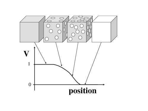
Figure 1: VOF with porous matter expression: For the consistency between the color function method and VOF-method, we consider each cell as a fictitious porous material whose volume ratio and open fraction are a value in $[0,1]$ without imposing any wall shear stress on fictitious surface of the porous parts in each cell. This expression represents purely geometrical effects.

As the convention in Reference [22], $V$ is also defined as a cellwise constant function. In the following examples, we will set $\epsilon_{0}$ to be $a$ or the unit cell basically. However we can also make it $\epsilon_{0}>a$ as for two-phase field. It means that for the case $\epsilon_{0}>a$, we consider each cell as a fictitious porous material whose volume ratio $V\in[0,1]$ without imposing any wall shear stress on the fictitious surface of the porous parts itself in each cell as in Figure 1. (As mentioned above, we set the wall shear stress $\hat{\tau}_{j}$ from the physical wall $\xi_{0}$. The porous parts are purely fictitious.) The region where $V$ is equal to 1 means the region where fluid freely exists whereas the region where $V$ vanishes means the region where existence of fluid is prohibited. The region with $V\in(0,1)$ is the intermediate region $(M_{0}\setminus L_{0}^{c})^{\circ}$. Here we emphasize that the fictitious porous in each cell brings purely geometrical effects to this model.

Then we could go on to consider the problem in consistency between VOF-method and $\xi_{0}$ function in the phase-field model. Let functions $f_{1}\equiv f$ and $f_{2}$ over ${\rm{supp}}(V)$ be defined by the relations,

$$\xi_{1}=Vf_{1},\quad\xi_{2}=Vf_{2},\quad f_{1}+f_{2}=1.$$

Further we also modify the open fraction $A$ in the VOF-method, which is defined over each face. We interpret $A$ as the open area of the fictitious porous material of each face of each cell, which also has a value in $[0,1]$ as in Figure 1. We also use the open area fraction $A$ of each face of each cell [22, 21]. For a face belonging to the cell whose $V=1$, $A$ is also equal to 1. Following the convention in discretization by Hirt [22], $A$ is regarded as an operator acting on the face-valued functions like

$$A\circ u\equiv Au=(A_{1}u^{1},A_{2}u^{2},A_{3}u^{3}),$$

$$(Au)^{1}=A_{1}u^{1},\quad(Au)^{2}=A_{2}u^{2},\quad(Au)^{3}=A_{3}u^{3}.\quad$$ (6.3)

Here we note that $A_{i}a^{2}$ implicitly appearing in (6.3) can be interpreted as a two-chain of homological base associated with a face of a cell. For example, for a velocity field $\mu:=u^{i}(x)dx^{i}$ defined over a cell in the continuous theory and a piece of the boundary element of the cell $A_{1}a^{2}$, the discretized $u^{1}$ defined over the face is given by

$$(Au)^{1}:=\frac{1}{a^{2}}\int_{A_{1}a^{2}}*\mu=A_{1}u^{1},$$

where $*$ is the Hodge star operator, i.e., $*\mu:=u^{1}(x)dx^{2}dx^{3}+u^{2}(x)dx^{3}dx^{1}+u^{3}(x)dx^{1}dx^{2}$. Thus the discretization (6.3) is very natural even from the point of view of the modern differential geometry.

Hence $\mathrm{div}(u)\equiv\nabla u$ reads $\nabla Au$ as the difference equation in VOF-method [22] and we employ this discretization method.

We give our algorithm to compute (6.1) precisely as follows. As a convention, we specify the quantities with “old” and “new” corresponding to the previous states and the next states at each time step respectively in the computation. In other words, we give the algorithm that we construct the next states using the previous data by regarding the current state as an intermediate state in the time step. We use the project-method [13, 15];

$$\begin{split}\mbox{I}&:\frac{\rho\tilde{{u}}-\rho{{u}}^{\mathrm{old}}}{\Delta t}=-({{u}}^{\mathrm{old}}\cdot\nabla)\rho{{u}}^{\mathrm{old}},\\ \mbox{II}&:\frac{{{u}}^{\mathrm{new}}-\tilde{{u}}}{\Delta t}=-\frac{1}{\rho}(\nabla p-{{K}}),\\ \mbox{III}&:\nabla{{u}}^{\mathrm{new}}=0.\\ \end{split}$$

The step I is the part of the advection of the velocity ${{u}}^{\mathrm{old}}$. In the step I, we define an intermediate velocity $\tilde{{u}}$ and after then, we compute ${{u}}^{\mathrm{new}}$ and $p$ in the steps II and III.

The time-development of $\rho$ is given by the equation,

$$f^{\mathrm{new}}=f^{\mathrm{old}}+\Delta t\nabla((A{{u}}^{\mathrm{old}})f^{\mathrm{old}}),$$

and

$$\rho=V(\rho_{1}f+\rho_{2}(1-f))$$

for the proper densities $\rho_{a}$ of $\xi_{a}$ $(a=1,2)$.

Even for the case that we can deal with multi-phase flow with large density difference, we evaluate its time-development. Precisely speaking, when we evaluate $\tilde{{u}}$, following the idea of Rudman [39] we employ the momentum advection $\tilde{{u}}$ of ${{u}}$,

$$\tilde{{u}}:=\frac{1}{\rho^{\mathrm{new}}}[\rho^{\mathrm{old}}{{u}}^{\mathrm{old}}-\Delta t({{u}}^{\mathrm{old}}\cdot\nabla)\rho^{\mathrm{old}}{{u}}^{\mathrm{old}}].$$

Our derivation of the Euler equation shows that the Rudman’s method is quite natural.

Following the conventional notation, the guessed-value of the velocity is denoted by ${{u}}^{*}$, which is the initial value for the steps in II and III. Let us define

$${{u}}^{*}:=\tilde{{u}}+\Delta t\frac{1}{\rho^{\mathrm{new}}}{{K}}(\rho^{\mathrm{old}},f^{\mathrm{old}},{{u}}^{\mathrm{old}}).$$

In order to evaluate the guessed velocity, we compute the force ${{K}}$ from (6.2) noting that $\mathrm{div}\tau$ and $\mathrm{div}\overline{\tau}$ read $\nabla A\tau$ and $\nabla A\overline{\tau}$ respectively.

Following the SMAC (Simplified-Marker-and-Cell) method [3, 13, 15], we numerically determine the new velocity ${{u}}^{\mathrm{new}}$ and the pressure $p$ in a certain boundary condition using the preconditioned conjugate gradient method (PCGM):

$$\begin{split}\mbox{(IIa) Evaluate }p\mbox{ using the PCGM}&:\frac{1}{\Delta t}\nabla(A\circ{{u}}^{*})=\nabla A\circ\frac{1}{\rho^{\mathrm{new}}}\nabla p,\\ \mbox{(IIb) By using }p\mbox{ determine }{{u}}^{\mathrm{new}}&:{{u}}^{\mathrm{new}}={{u}}^{*}-\Delta t\frac{1}{\rho^{\mathrm{new}}}\nabla p.\\ \end{split}$$

More precisely speaking, (III) $\nabla(A\circ{{u}}^{\mathrm{new}})=0$ means that we numerically solve the Poisson equation,

$$\nabla\left(A\Delta t\frac{1}{\rho^{\mathrm{new}}}\nabla p\right)=\nabla(A\circ{{u}}^{*}).$$

Then we obtain ${{u}}^{\mathrm{new}}$, which obviously satisfies (III) $\nabla(A\circ{{u}}^{\mathrm{new}})=0$, which is known as the Hodge decomposition method [3, 13, 14] as mentioned in Remark 1.

Following the algorithm, we computed the two-phase flow with a wall and triple junctions. We illustrate two examples of the numerical solutions of the triple junction problems as follows.

6.1 Example 1

Here we show a computation of a capillary problem, or the meniscus oscillation, in Figure 2. We set two liquids in a parallel wall with the physical parameters; $\eta_{1}=\eta_{2}=0.1$[cp], $\rho_{1}=\rho_{2}=1.0$[pg/${\mu\mathrm{m}}^{3}$], $\sigma_{1}=3.349$[pg/$\mu$sec²], $\sigma_{2}=46.651$[pg/$\mu$sec²].

We used ${\mathcal{L}}:=12[{\mu\mathrm{m}}]\times 0.5[{\mu\mathrm{m}}]\times 16[{\mu\mathrm{m}}]$ lattice whose unit length $a$ is $0.125[{\mu\mathrm{m}}]$. The first liquid exists in the down side and the second liquid does in the upper side in the region $10[{\mu\mathrm{m}}]\times 0.5[{\mu\mathrm{m}}]\times 15[{\mu\mathrm{m}}]$ surrounded by the wall and the boundaries with the boundary conditions. As the boundary conditions, at the upper side from the bottom of the wall by $15[{\mu\mathrm{m}}]$, we fix the constant pressure as $100$[KPa] and, along $x^{2}$-direction, we set the periodic boundary condition.

We set $\epsilon_{12}=\epsilon_{0}=1$ mesh for the intermediate regions, at least, as its initial condition. Each time interval is 0.001 [$\mu$sec].

As the initial state, we start the state that the fluid surface is flat as in Figure 2 (a) and the first liquid exists in the box region $10[{\mu\mathrm{m}}]\times 0.5[{\mu\mathrm{m}}]\times 7.0[{\mu\mathrm{m}}]$, which is not stable. Due to the surface tension, it moves and starts to oscillate but due to viscosity, the oscillation decays. Though we did not impose the contact angle as a geometrical constraint, the dynamics of the contact angle was calculated due to a balance between the kinematic energy and the potential energy or the surface energy. The oscillation converged to the stable shape with the proper contact angle, which is given by

$$\cos\varphi=\frac{\sigma_{2}-\sigma_{1}}{\sigma_{2}+\sigma_{1}}\equiv\frac{\sigma_{02}-\sigma_{01}}{\sigma_{12}}.$$ (6.4)

The angle given by $\sigma$’s are designed as $30$ [degree] whereas it in the numerical experiment in Figure 2 is a little bit larger than $30$ [degree], though it is very difficult to determine it precisely. However since we could tune the parameters $\sigma$’s so that we obtain the required state, our formulation is very practical.

Due to the numerical diffusions and others, the thickness of the intermediate regions changes in the time development and also depends on the positions of the interfaces, even though it is fixed the same at the initial state. However we consider that it is thin enough to evaluate the physical system since the contact angle is reasonably estimated.

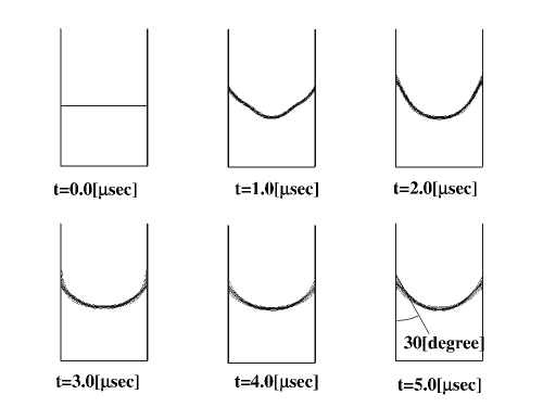
Figure 2: The meniscus oscillation: Each figure shows the time development.

6.2 Example 2

This example is on the computations of the contact angles for different surface tension coefficients displayed in Figure 3.

Even in this case, in order to see the difference between the designed contact angle and computed one, we go on to handle two-dimensional symmetrical problems though we used three-dimensional computational software. In other words, we set that $x^{2}$-direction is periodic.

Since the contact angle $\varphi$ in our convention is given by the formula (6.4). By setting $\sigma$’s

$$\frac{\sigma_{1}}{\sigma_{2}}=\frac{1-\cos\varphi}{1+\cos\varphi},$$

for given the contact angle $\varphi$, we computed five triple junction problems without any geometrical constraints; each $\sigma$ is given in the caption in Figure 3. The other physical parameters are given by $\eta_{1}=\eta_{2}=0.1$[cp] and $\rho_{1}=\rho_{2}=1.0$[pg/${\mu\mathrm{m}}^{3}$].

In this computation we used a $240\times 4\times 112$ lattice whose unit length $a$ is $0.125[{\mu\mathrm{m}}]$; $\Omega=30[{\mu\mathrm{m}}]\times 0.5[{\mu\mathrm{m}}]\times 14[{\mu\mathrm{m}}]$. We set the flat layer as a wall by thickness $3[{\mu\mathrm{m}}]$ from the bottom of $\Omega$ along the $z$-axis. As the boundary conditions, at the upper side from the bottom of the wall by $9[{\mu\mathrm{m}}]$, we fix the constant pressure as $100$[KPa].

As the initial state for each computation. we set a semicylinder with radius $5[\mu m]$ in the flat wall like Figure 3 (d). We also set $\epsilon_{12}=\epsilon_{0}=1$ mesh for the intermediate regions. Each time step also corresponds to 0.001 [sec].

Due to the viscosity, after time passes sufficiently $50[\mu$sec], the static solutions were obtained as illustrated in Figure 3, which recover the contact angles under our approximation within good agreements.

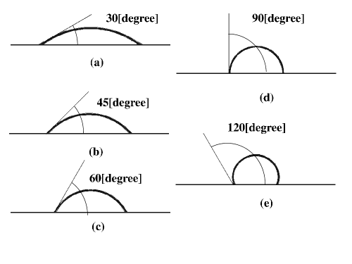
Figure 3: The different contact angles are illustrated due to the different surface energy: By fixing $\sigma_{1}=1.0000$[pg/$\mu$sec³], (a): $\varphi=30$ [degree], $\sigma_{2}=13.9282$[pg/$\mu$sec³], (b): $\varphi=45$ [degree], $\sigma_{2}=5.8284$[pg/$\mu$sec³], (c): $\varphi=60$ [degree], $\sigma_{2}=3.0000$[pg/$\mu$sec³], (d): $\varphi=90$ [degree], $\sigma_{2}=1.0000$[pg/$\mu$sec³], and (e): $\varphi=120$ [degree], $\sigma_{2}=0.3333$[pg/$\mu$sec³].

7 Summary

By exploring an incompressible fluid with a phase-field geometrically [1, 4, 18, 25, 28, 32, 37], we reformulated the expression of the surface tension for the two-phase flow found by Lafaurie, Nardone, Scardovelli, Zaleski and Zanetti [31] as a variational problem. We reproduced the Euler equation of two-phase flow (4.11) following the variational principle of the action integral (4.7) in Proposition 10.

The new formulation along the line of the variational principle enabled us to extend (4.11) to that for the multi-phase ($N$-phase, $N\geq 2$) flow. By extending (4.11), we obtained the novel Euler equation (5.14) with the surface tension of the multi-phase fields in Theorem 2 from the action integral of Theorem 1 as the conservation of momentum in the sense of Noether’s theorem. The variational principle for the infinite dimensional system in the sense of References [1, 4, 18] gives the equation of motion of multi-phase flow controlled by the small parameter ${\epsilon_{\xi}}$ without any geometrical constraints and any difficulties for the singularities at multiple junctions.

For the static case, we gave governing equations (5.6), (5.7) and (5.10) which generate the locally constant mean curvature surfaces with triple junctions by controlling a parameter ${\epsilon_{\xi}}$ to avoid these singularities. As the solutions of (4.4) has been studied well as the constant mean curvature surfaces for last two decades [17, 19, 20, 47], our extended equations (5.6), (5.7) and (5.10) might shed new light on treatment of singularities of their extended surfaces, or a set of locally constant mean curvature surfaces. (Even though we need an interpretation of our scheme, for example, it can be applied to a soap film problem with triple junction.) It implies that our method might give a method of resolutions of singularities in the framework of analytic geometry.

By specifying the problem of the multi-phase flow to the contact angle problems at triple junctions with a static wall, we obtained the simpler Euler equation (5.16) in Theorem 3. Using the VOF method [22, 21], we showed two examples of the numerical computations in Section 6. In our computational method, for given surface tension coefficients, the contact angle is automatically generated by the surface tension without any geometrical constraints and any difficulties for the singularities at triple junctions. The computations were very stable. It means that the computations did not collapse nor behave wildly for every initial and the boundary conditions.

In our theoretical framework, we have unified the infinite dimensional geometry or an incompressible fluid dynamics governed by ${\rm{IFluid}}(\Omega\times T)$, and the ${\epsilon_{\xi}}$-parameterized low dimensional geometry with singularities given by the multi-phase fields. We obtained all of equations following the same variational principle. We naturally reproduced the Laplace equations, (4.4) and (5.6), and obtained their generalizations (4.8), (5.6), (5.7), (5.13) and (5.10), and the Euler equations, (4.11), (5.14), and (5.16) in Proposition 10 and Theorems 2 and 3. These equations are derived from the same action integrals by choosing the physical parameters. In the sense of References [1, 5, 10], it implies that we gave geometrical interpretations of the multi-phase flow. Even though the phase-field model has the artificial intermediate regions with unphysical thickness ${\epsilon_{\xi}}$, our theory supplies a model which shows how to evaluate their effects on the surface tension forces, from geometrical viewpoints. The key fact of the model is that we express the low-dimensional geometry in terms of the infinite-dimensional vector spaces, or global functions $\xi$’s which have natural ${\rm{Diff}}$ and ${\rm{SDiff}}$ actions. Thus we can treat them in the framework of infinite dimensional Lie group [4, 18, 38] to consider its Euler equation. It is contrast to the level-set method; in analytic geometry and algebraic geometry, zeros of a function expresses a geometrical object and thus the level-set method is so natural from the point of view. However as mentioned in Section 2.1, the level-set function cannot be a global functions as ${\mathcal{C}}^{\infty}(\Omega)$ and thus it is difficult to handle the method in the framework of the infinite dimensional Lie group ${\rm{SDiff}}(\Omega)$.

As our approach gives a resolution of the singularities by a parameter ${\epsilon_{\xi}}$, in future we will explore topology changes, geometrical objects with singularities and so on, more concretely in our theoretical framework. When ${\epsilon_{\xi}}$ approaches to zero, we need more rigorous arguments in terms of hyperfunctions [26] but we conjecture that our results would be correct for the vanishing limit of ${\epsilon_{\xi}}$ because the Heaviside function is expressed by $\displaystyle{\theta(q)=\lim_{{\epsilon_{\xi}}\to 0}\frac{1}{\pi}\tan^{-1}\left(\frac{q}{{\epsilon_{\xi}}}\right)}$ in the Sato hyperfunction theory, which could be basically identified with $\xi(q)$ of the finite ${\epsilon_{\xi}}$. Since an application of the Sato hyperfunction theory to fluid dynamics was reported by Imai on vortex layer and so on [29], we believe that this approach might give another collaboration between pure mathematics and fluid mechanics.

Acknowledgements:

This article is written by the authors in memory of their colleague, collaborator and leader Dr. Akira Asai who led to develop this project. The authors are also grateful to Mr. Katsuhiro Watanabe for critical discussions and to the anonymous referee for helpful and crucial comments.

Shigeki Matsutani

Analysis technology center, Canon Inc.

3-3-20, Shimomaruko, Ota-ku, Tokyo 146-8501, Japan

matsutani.shigeki@canon.co.jp,

Kota Nakano

Analysis technology center, Canon Inc.

3-3-20, Shimomaruko, Ota-ku, Tokyo 146-8501, Japan

Katsuhiko Shinjo

Analysis technology center, Canon Inc.

3-3-20, Shimomaruko, Ota-ku, Tokyo 146-8501, Japan

References

- [1] V. I. Arnol’d, Mathematical methods of classical mechanics, 2nd ed., GTM 60 (Springer, Berlin, 1989) .
- [2] V. I. Arnol’d, V. V. Goryunov, O. V. Lyashko, and V. A. Vasil’ev, Singularity Theory I, , translated by A. Iacob, (Springer, Berlin, 1998) .
- [3] A. A. Amsden and F. H. Harlow, A simplified MAC technique for incompressible fluid flow calculations, J. Comp. Phys. 6 (1970) pp.322-330.
- [4] V. I. Arnold and B. A. Khesin, Topological Methods in Hydrodynamics (Applied Mathematical Sciences), 2nd. ed., (Springer, Berlin, 1997) .
- [5] R. Abraham and J. Marsden, Foundation of Mechanics, (AMS Chelsea Publishing, New York, 1987) .
- [6] S. Albeverio and B. Ferrario, Some Methods of Infinite Dimensional Analysis in Hydrodynamics: An Introductions, Lecture Notes in Mathematics: SPDE in Hydrodynamic: Recent Progress and Prospects, (2008) pp.1-50.
- [7] E. Aulisa, S. Manservisi and R. Scardovelli, A novel representation of the surface tension force for two-phase flow with reduced spurious current, Comp. Methods Appl Mech. Engrg. 195 (2006) pp.6239-6257.
- [8] K. Beyer, and M. Günther, On the Cauchy Problem for a Capillary Drop. Part I: Irrotational Motion, Math. Methods. Appl. Sci. 21 (1998) pp.1149-1183.
- [9] Y. Brenier, Generalized solutions and hydrostatic approximation of the Euler equations, Physica D 237 (2008) pp.1982-1988.
- [10] R. Bryant, P. Griffiths, and D. Grossman, Exterior differential systems and Euler-Lagrange partial differential equations, (Univ. Chicago, Chicago, 2003) .
- [11] J. U. Brakbill, D. B. Kothe, and C. Zemach, A Continuum Method for Modeling Surface Tension, J. Comp. Phys. 100 (1992) pp.335-354.
- [12] A. Caboussat, A numerical method for the simulation of free surface flows with surface tension, Comp. Fluids 35 (2006) pp.1205-1216.
- [13] A. J. Chorin, Numerical solution of the Navier-Stokes equations, Math. Comp. 22 (1968) pp.745-762.
- [14] A. J. Chorin and J. E. Marsden, A Mathematical Introduction to Fluid Mechanics, 3rd ed., (Springer, 1992) .
- [15] T. J. Chung, Computational Fluid Dynamics, (Cambridge University Press, 2002) .
- [16] L.P. Eisenhart, A Treatise on the Differential Geometry of Curves and Surfaces, (Ginn and Company, 1909) .
- [17] L. C. Evans and J. Spruck , Motion of level sets by mean curvature. I, J. Diff. Geom. 33 (1991) pp.635-681.
- [18] D. Ebin and J. Marsden, Groups of diffeomorphisms and the motion of an incompressible fluid, Ann. Math. 92 (1970) pp.102-163.
- [19] A. P. Fordy and J. C. Wood, (eds.) Harmonic maps and integrable systems, (Friedrich Viewweg and Sohn Verlag, Berlin, 1994) .
- [20] M. Guest, R. Miyaoka, Y. Onihta, (eds.) Surveys on Geometry and Integrable systems, Advanced Studies in Pure Math. 51 (2008) .
- [21] C. W. Hirt and B. D. Nichols, Volume of Fluid (VOF) Method for Dynamics of Free Boundaries, J. Comp. Phys. 39 (1981) pp.201-225.
- [22] C. W. Hirt, Volume-fraction techniques: powerful tools for wind engineering, J. Wind Engineering and Industrial Aerodynamics 46 & 47 (1993) pp.327-338.
- [23] C. Itzykson and J. Zuber, Quantum Field Theory, (McGraw-Hill, New York, 1980) .
- [24] D. Jacqmin, Calculation of Two-Phase Navier-Stokes Flows Using Phase-Field Modeling, J. Comp. Phys. 155 (1999) pp.96-127.
- [25] T. Kambe, Variational formulation of ideal fluid flows according to gauge principle, Fluid Dynamics Research 40 (2008) pp.399-426.
- [26] M. Kashiwara, T. Kawai, T. Kimura, Foundations of algebraic analysis, translated by G. Kato, (Princeton, Princeton Univ., 1986) .
- [27] S. Kobayashi and K. Nomizu, Foundations of Differential Geometry vol. 1, 2, (Weily, New York, 1996) .
- [28] T. Kori, Hamilton form of Yang-Mills equation, RIMS Kokyuroku (Kyoto Univ) 1408 (2004) pp.110-122 (in Japanese);
- [29] I Imai, Applied Hyperfunction Theory, (Kluwer, Dordrecht, 1992) .
- [30] L. D. Landau, E. M Lifshitz, Fluid Mechanics (Course of Theoretical Physics) 2nd Eds., Butterworth-Heinemann; (1987/01) Foundations of Differential Geometry vol. 1, 2, (Butterworth-Heinemann, New York, 1987) .
- [31] B. Lafaurie, C. Nardone, R. Scardovelli, S. Zaleski, G. Zanetti, Modelling Merging and Fragmentation in Multiphase Flows with SURFER, J. Comp. Phys. 113 (1994) pp.134-147.
- [32] J. Marsden and A. Weinstein, Codajoint orbits, vortices, and clebsch variables for incompressible fluids, Physica 7D (1983) pp.305-323.
- [33] K. Maeda, and U. Miyamoto, Black hole-black string phase transitions from hydrodynamics, J. High Energy Phys. 03 (2009) pp.066.
- [34] S. Matsutani, A Generalized Weierstrass representation for a submanifold in arising from the submanifold Dirac operator, Adovanced Studies in Pure Math. 51 (2008) pp.259-283.
- [35] S. Matsutani, Sheaf-theoretic investigation of CIP-method, App. Math. Comp. 217 (2010) pp.568-579.
- [36] M. Nakahara, Geometry, Topology and Physics, 2nd ed., (IOP Publ., Bristol, 2003) .
- [37] F. Nakamura, Y. Hattori, and T. Kambe, Geodesics and curvature of a group of diffeomorphisms and motion of an ideal fluid, J. Phys. A: Math. Gen. 25 (1992) pp.L45-L50.
- [38] H. Omori, Infinite-dimensional Lie Groups, (Amer. Math. Soc., New York, TMM158 1997) .
- [39] M. Rudman, A volume-tracking method for incompressible multifluid flows with large density variations, Int. J. Numer. Meth. Fluids 28 (1998) pp.357-378.
- [40] J. Shatah and C. Zeng, A Priori Estimates for Fluid Interface Problems, Comm. Pure Appl. Math. LXI (2008) pp.848-876.
- [41] R. Schmid, Infinite Dimensional Lie Groups with Applications to Mathematical Physics, J. of Geom. and Symm. Phys. 1 (2004) pp.1-67. 33,11 末尾
- [42] J. A. Sethian, Level Set Methods and Fast Marching Methods: Evolving Interfaces in Computational Geometry, Fluid Mechanics, Computer Vision, and Materials Science 2nd, (Cambridge, Cambridge, 1999) .
- [43] S. Shkoller, Analysis on groups of diffeomorphisms of manifolds with boundary and the averaged motion of fluid, J. Diff. Geom. 55 (2000) pp.145-191.
- [44] A. Shnirelman, Microglobal Analysis of the Euler Equations, J. Math. Fluid Mech. 7 (2005) pp.S387-S396.
- [45] H-K Zhao, B Merriman, S Osher and L Wang, Capturing the Behavior of Bubbles and Drops Using the Variational Level Set Approach, J. Comp. Phys. 143 (1998) pp.495-518.
- [46] H-K Zhao, T Chan, B Merriman and S Osher, A Variational Level Set Approach to Multiphase Motion, J. Comp. Phys. 127 (1996) pp.179-195.
- [47] I. A. Taimanov, Two-dimensional Dirac operator and theory of surface, Russian Math. Survey 61 (2006) pp.79-159.
- [48] K. Yoshida, Functional Analysis, sixth-eds (Springer-Kinokuniya, Tokyo, 1970) .
- [49] C. Vizman, Geodesic Equations on Diffeomorphism Groups, SIGMA 4 (2008) pp.030, 22 pages.