An EM Algorithm for Continuous-time Bivariate Markov Chains

Abstract

We study properties and parameter estimation of finite-state homogeneous continuous-time bivariate Markov chains. Only one of the two processes of the bivariate Markov chain is observable. The general form of the bivariate Markov chain studied here makes no assumptions on the structure of the generator of the chain, and hence, neither the underlying process nor the observable process is necessarily Markov. The bivariate Markov chain allows for simultaneous jumps of the underlying and observable processes. Furthermore, the inter-arrival time of observed events is phase-type. The bivariate Markov chain generalizes the batch Markovian arrival process as well as the Markov modulated Markov process. We develop an expectation-maximization (EM) procedure for estimating the generator of a bivariate Markov chain, and we demonstrate its performance. The procedure does not rely on any numerical integration or sampling scheme of the continuous-time bivariate Markov chain. The proposed EM algorithm is equally applicable to multivariate Markov chains.

Keywords:

Parameter estimation, EM algorithm, Continuous-time bivariate Markov chain, Markov modulated processes

1 Introduction

We consider the problem of estimating the parameter of a continuous-time finite-state homogeneous bivariate Markov chain. Only one of the two processes of the bivariate Markov chain is observable. The other is commonly referred to as the underlying process. We do not restrict the structure of the generator of the bivariate Markov chain to have any particular form. Thus, simultaneous jumps of the observable and underlying processes are possible, and neither of these two processes is necessarily Markov. In [25], a continuous-time bivariate Markov chain was used to model delays and congestion in a computer network, and a parameter estimation algorithm was proposed. The model was motivated by the desire to capture correlations observed empirically in samples of network delays. A continuous-time multivariate Markov chain was used to model ion channel currents in [3].

The bivariate Markov chain generalizes commonly used models such as the batch Markovian arrival process (BMAP) [5, 13], the Markov modulated Markov process (MMMP) [8], and the Markov modulated Poisson process (MMPP) [10, 20, 21, 18]. In the BMAP, for example, the generator is an infinite upper triangular block Toeplitz matrix. In the MMMP and MMPP, the generator is such that no simultaneous jumps of the underlying and observable processes are allowed. In addition, the underlying processes in all three examples are homogeneous continuous-time Markov chains.

We develop an expectation-maximization (EM) algorithm for estimating the parameter of a continuous-time bivariate Markov chain. The proposed EM algorithm is equally applicable to multivariate Markov chains. An EM algorithm for the MMPP was originally developed by Rydén[21]. Using a similar approach, EM algorithms were subsequently developed for the BMAP in [5, 13] and the MMMP in [8]. The EM algorithm developed in the present paper also relies on Rydén’s approach. It consists of closed-form, stable recursions employing scaling and Van Loan’s approach for computation of integrals of matrix exponentials [24], along the lines of [18, 8].

In the parameter estimation algorithm of [25], the continuous-time bivariate Markov chain is first sampled and the transition matrix of the resulting discrete-time bivariate Markov chain is estimated using a variant of the Baum algorithm [4]. The generator of the continuous-time bivariate Markov chain is subsequently obtained from the transition matrix estimate. As discussed in [17], this approach may lead to ambiguous estimates of the generator of the bivariate Markov chain, and in some cases it will not lead to a valid estimate. Moreover, the approach does not allow structuring of the generator estimate since it is obtained as a byproduct of the transition matrix estimate. The EM algorithm developed in this paper estimates the generator of the bivariate Markov chain directly from a sample path of the continuous-time observable process. This leads to a more accurate computationally efficient estimator which is free of the above drawbacks.

The remainder of this paper is organized as follows. In Section 2, we discuss properties of the continuous-time bivariate Markov chain and develop associated likelihood functions. In Section 3, we develop the EM algorithm. In Section 4, we discuss the implementation of the EM algorithm and provide a numerical example. Concluding remarks are given in Section 5.

2 Continuous-time Bivariate Markov Chain

Consider a finite-state homogeneous continuous-time bivariate Markov chain

$$Z=(X,S)=\{(X(t),S(t)),~{}t\geq 0\},$$ (1)

defined on a standard probability space, and assume that it is irreducible. The process $S=\{S(t),t\geq 0\}$ is the underlying process with state space of say $\{a_{1},\ldots,a_{r}\}$, and $X=\{X(t),t\geq 0\}$ is the observable process with state space of say $\{b_{1},\ldots,b_{d}\}$. The orders $r$ and $d$ are assumed known. We assume without loss of generality that $a_{i}=i$ for $i=1,\ldots,r$ and $b_{l}=l$ for $l=1,\ldots,d$. The state space of $Z$ is then given by $\{1,\ldots,d\}\times\{1,\ldots,r\}$. Neither $X$ nor $S$ need be Markov. Necessary and sufficient conditions for either process to be a homogeneous continuous-time Markov chain are given in [3, Theorem 3.1]. With probability one, all sample paths of $Z$ are right-continuous step functions with a finite number of jumps in any finite interval [1, Theorem 2.1].

The bivariate Markov chain is parameterized by a generator matrix

$$H=\{h_{ln}(ij),~{}l,n=1,\ldots d;i,j=1,\ldots r\},$$ (2)

where the set of joint states $\{(l,i)\}$ is ordered lexicographically. With $P(\cdot)$ denoting the probability measure on the given space,

$$h_{ln}(ij)=\lim_{\epsilon\rightarrow 0}\frac{1}{\epsilon}P(Z(t+\epsilon)=(n,j)\mid Z(t)=(l,i)),$$ (3)

for $(l,i)\neq(n,j)$. The generator matrix can be expressed as a block matrix $H=\{H_{ln},~{}l,n=1,\ldots,d\}$, where $H_{ln}=\{h_{ln}(ij),~{}i,j=1,\ldots,r\}$ are $r\times r$ matrices. The number of independent scalar values that constitute the generator $H$ is at most $rd(rd-1)$. Since none of the rows of $H$ is identically zero, the submatrix $H_{ll}$, $l\in\{1,\ldots,d\}$, is strictly diagonally dominant, i.e.,

$$-h_{ll}(ii)=\sum_{(n,j):(n,j)\neq(l,i)}h_{ln}(ij)>\sum_{j:j\neq i}h_{ll}(ij),$$ (4)

for all $i=1,\ldots,r$, and thus, $H_{ll}$ is nonsingular [23, p. 476].

Clearly, the observable process $X(t)$ is a deterministic function of the bivariate Markov chain $Z(t)$. Conversely, the pair consisting of a univariate Markov chain together with a deterministic function of that chain is a bivariate Markov chain (see [19]).

2.1 Density of observable process

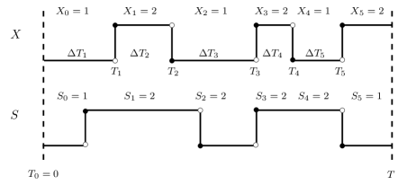
Figure 1: Example sample path of $Z=(X,S)$.

Assume that the observable process $X$ of a bivariate Markov chain $Z=(X,S)$ starts from some state $X_{0}$ at time $T_{0}=0$ and jumps $N$ times in $[0,T]$ at $0<T_{1}<T_{2}<\cdots<T_{N}\leq T$. Let $X_{k}=X(T_{k})$ denote the state of $X$ in the interval $[T_{k},T_{k+1})$ for $k=1,2,\ldots,N-1$ and let $X_{N}$ denote the state of $X$ in the interval $[T_{N},T]$. This convention differs slightly from that used in [8], where $X_{k}\triangleq X(T_{k-1})$, $k=1,\ldots,N+1$. Define $S_{k}=S(T_{k})$ to be the state of $S$ at the jump time $T_{k}$ of $X$. Let $Z_{k}=Z(T_{k})=(X_{k},S_{k})$. Let $\Delta T_{k}=T_{k}-T_{k-1}$ denote the dwell time of $X$ in state $X_{k-1}$ during the interval $[T_{k-1},T_{k})$, $k=1,\ldots,N$. We denote realizations of $X_{k}$, $S_{k}$, $Z_{k}$, $T_{k}$, and $\Delta T_{k}$ by $x_{k}$, $s_{k}$, $z_{k}$, $t_{k}$, and $\Delta t_{k}$, respectively. Figure 1 depicts a sample path of a bivariate Markov chain $Z=(X,S)$ for which $N=5$, $r=d=2$, $a_{1}=1$, $a_{2}=2$, $b_{1}=1$, and $b_{2}=2$. From the figure, we see that the sequence $\{Z_{k}\}$ is given by

$$\{(1,1),(2,2),(1,2),(2,2),(1,2),(2,1)\}.$$ (5)

Note that in Figure 1, the processes $X$ and $S$ jump simultaneously at times $T_{3}$ and $T_{5}$.

The bivariate Markov chain $Z$ is a pure-jump Markov process and is therefore strong Markov (see [26, Section 4-1]) Using the strong Markov property of $Z$, it follows that

$$P( Z_{k+1}=z,\Delta T_{k+1}\leq\tau\mid Z_{0},\ldots,Z_{k};T_{0},\ldots,T_{k})$$

$$=P(Z_{k+1}=z,\Delta T_{k+1}\leq\tau\mid Z_{k})$$ (6)

for all $z\in\{1,\ldots,d\}\times\{1,\ldots,r\}$; $\tau\geq 0$; and $k=0,1,2,\ldots$. Therefore, $\{(Z_{k},T_{k})\}$ is a Markov renewal process (see [6]). Since the observable process $X$ can be represented in an equivalent form as $\{(X_{k},T_{k})\}$, it follows that the density of $X$ in $[0,T_{N}]$ may be obtained from the product of transition densities of $\{(Z_{k},T_{k})\}$. If $T>T_{N}$, an additional term is required to obtain the density of $X$ in $[0,T]$, as will be specified shortly.

Assuming a stationary bivariate Markov chain, the transition density of $\{(Z_{k},T_{k})\}$ follows from the density corresponding to

$$P(Z(\tau)=(n,j),T_{1}\in[\tau,\tau+d\tau)\mid Z(0)=(l,i)),$$ (7)

for $l\neq n$, which we denote by $f_{ij}^{ln}(\tau)$. Let $f^{ln}(\tau)=\{f_{ij}^{ln}(\tau),~{}i,j=1,\ldots,r\}$ denote the transition density matrix of $\{(Z_{k},T_{k})\}$. When $\tau$ does not coincide with a jump time of the observable process, the transition probability

$$\bar{f}^{l}_{ij}(\tau)=P(S(\tau)=j,T_{1}>\tau\mid X(0)=l,S(0)=i)$$ (8)

is also required. Let $\bar{f}^{l}(\tau)=\{\bar{f}^{l}_{ij}(\tau),~{}i,j=1,\ldots,r\}$ denote the corresponding transition matrix. The following proposition gives explicit forms for $f^{ln}(\tau)$ and $\bar{f}^{l}(\tau)$.

Proposition 1.

For $\tau\geq 0$,

$$f^{ln}(\tau)=e^{H_{ll}\tau}H_{ln},~{}~{}l\neq n,$$ (9)

and

$$\bar{f}^{l}(\tau)=e^{H_{ll}\tau}.$$ (10)

Furthermore,

$$P(Z_{k+1}=(n,j)\mid Z_{k}=(l,i))=\left[-H_{ll}^{-1}H_{ln}\right]_{ij}.$$ (11)

Proof.

Following an argument similar to that given in [11, 8], the density $f_{ij}^{ln}(t)$ satisfies the following equation:

$$f_{ij}^{ln}(\tau)=h_{ln}(ij)e^{h_{ll}(ii)\tau}+e^{h_{ll}(ii)\tau}\!\int_{0}^{\tau}\!e^{-h_{ll}(ii)t}\sum_{k\neq i}h_{ll}(ik)f_{kj}^{ln}(t)dt.$$ (12)

Differentiating both sides of (12) with respect to $t$ and simplifying, it follows that

$$\frac{df_{ij}^{ln}(\tau)}{d\tau}=h_{ll}(ii)f_{ij}^{ln}(\tau)+\sum_{k\neq i}h_{ll}(ik)f_{kj}^{ln}(\tau)=\sum_{k}h_{ll}(ik)f_{kj}^{ln}(t\tau).$$ (13)

Therefore,

$$\frac{df^{ln}(\tau)}{d\tau}=H_{ll}f^{ln}(\tau)$$ (14)

with initial condition $f^{ln}(0)=H_{ln}$ from (12). Hence, (9) follows. Integrating (9) from $0$ to $\infty$ gives (11).

The transition probability $\bar{f}^{l}_{ij}(\tau)$ satisfies an equation similar to (12) except that the first term on the right-hand side is replaced by $e^{h_{ll}(ii)\tau}\delta_{ij}$. This change only affects the initial condition, viz., $\bar{f}^{l}(0)=I$, where $I$ denotes the identity matrix. Hence, (10) follows. ∎

To simplify notation in the sequel, we shall use $P(\cdot)$ to denote not only a probability measure, but also a density, as appropriate (cf. [21, 8]). The exact meaning of expressions involving $P(\cdot)$ should be clear from the context. In particular, all null probabilities are to be interpreted in the density sense. The density of $X$ in $[0,T]$ depends on the initial state probabilities $\mu_{x_{0}}(i)=P(X_{0}=x_{0},S_{0}=i)$, $i=1,\ldots,r$. Let

$$\mu_{x_{0}}=\{\mu_{x_{0}}(1),\mu_{x_{0}}(2),\ldots,\mu_{x_{0}}(r)\}$$ (15)

denote the initial state distribution. Using the Markov renewal property of $\{(Z_{k},T_{k})\}$, the density of $X$ in $[0,T]$ can be expressed as

$$P(X(t),0\leq t\leq T)=\mu_{x_{0}}\left\{\prod_{k=1}^{N}f^{x_{k-1}x_{k}}(\Delta t_{k})\right\}\bar{f}^{x_{N}}(T-t_{N})\mbox{\boldmath$1$},$$ (16)

where $1$ denotes a column vector of all ones. This expression will be used in Section 3 to develop the EM recursions.

2.2 Forward-backward recursions

The density in (16) can be evaluated using forward and backward recursions. The forward density is defined by the row vector

$$L(k) =\{P(X(t),0\leq t\leq t_{k},S_{k}=i),~{}i=1,\ldots,r\},$$ (17)

for $k=0,1,\ldots,N$. The forward recursion is given by

$$L(0) =\mu_{x_{0}},$$

$$L(k) =L(k-1)f^{x_{k-1}x_{k}}(\Delta t_{k}).$$ (18)

The backward density is defined by the column vector

$$R(k) =\{P(X(t),t_{k-1}<t\leq T\mid X_{k-1}=x_{k-1},S_{k-1}=i),~{}~{}i=1,\ldots,r\}^{\prime},$$

for $k=N\!+\!1,N,\ldots,1$, where ^′ denote matrix transpose. The backward recursion is given by

$$R(N+1) =\bar{f}^{x_{N}}(T-t_{N})\mbox{\boldmath$1$},$$

$$R(k) =f^{x_{k-1}x_{k}}(\Delta t_{k})R(k+1).$$ (19)

From (16)–(19), the density of the observable process in $[0,T]$ is given by

$$P(X(t),0\leq t\leq T)=L(k)R(k+1),~{}~{}~{}~{}k=0,\ldots,N.$$ (20)

To ensure numerical stability, it is necessary to scale the above recursions. Using an approach similar to that developed in [18], the scaled forward recursion is given by

$$\tilde{L}(0) =\mu_{x_{0}},$$

$$\tilde{L}(k) =\frac{\tilde{L}(k-1)f^{x_{k-1}x_{k}}(\Delta t_{k})}{c_{k}},~{}k=1,\ldots,N,$$ (21)

where

$$c_{k}\triangleq\tilde{L}(k-1)f^{x_{k-1}x_{k}}(\Delta t_{k})\mbox{\boldmath$1$},~{}~{}~{}k=1,\ldots,N.$$ (22)

The scaled backward recursion is given by

$$\tilde{R}(N\!+\!1) \!=\!\bar{f}^{x_{N}}(T-t_{N})\mbox{\boldmath$1$},$$

$$\tilde{R}(k) \!=\!\frac{f^{x_{k\!-\!1}x_{k}}(\Delta t_{k})\tilde{R}(k\!+\!1)}{c_{k}},~{}k=1,\ldots,N.$$ (23)

Clearly, $\tilde{L}(0)=L(0)$ and $\tilde{R}(N\!+\!1)=R(N\!+\!1)$. For $k=1,\ldots,N$, one can show straightforwardly that the scaled and unscaled iterates of the forward and backward recursions are related by

$$\tilde{L}(k)=\frac{L(k)}{\prod_{m=1}^{k}c_{m}}~{}\mbox{and}~{}\tilde{R}(k)=\frac{R(k)}{\prod_{m=k}^{N}c_{m}}.$$ (24)

From (24) and (17), one sees that for $k=1,\ldots,N$, the scaled forward vector $\tilde{L}(k)$ can be interpreted as the probability distribution of the underlying process $S$ at time $T_{k}$ conditioned on the observable sample path up to and including time $t_{k}$:

$$\tilde{L}(k)=\left\{P(S_{k}=i\mid X(t),0\leq t<t_{k}),i=1,\ldots,r\right\}.$$ (25)

Thus, the density of $X$ up to and including the $N$th jump can be expressed as the product of the scaling constants as follows:

$$P(X(t),0\leq t\leq t_{N})=L(N)\mbox{\boldmath$1$}=\left(\prod_{k=1}^{N}c_{k}\right)\tilde{L}(N)\mbox{\boldmath$1$}=\prod_{k=1}^{N}c_{k}.$$ (26)

Therefore, the log-likelihood of the observed sample path is given by

$$\mathcal{L}=\sum_{k=1}^{N}\log c_{k}.$$ (27)

The above forward and backward recursions can be generalized to apply to any time $t$ between jump times of the observable process. In particular, for $t\in[t_{k},t_{k+1})$, consider the row vector

$$\tilde{\ell}(t) =\left\{P(S(t)=i\mid X(\tau),0\leq\tau\leq t),~{}i=1,\ldots,r\right\}.$$ (28)

It follows that

$$\tilde{\ell}(t)=\frac{L(k)\bar{f}^{x_{k}}(t-t_{k})}{L(k)\bar{f}^{x_{k}}(t-t_{k})\mbox{\boldmath$1$}}.$$ (29)

A similar result was derived by [19].

2.3 Properties

The observable process $X$ is conditionally Markov given $S$, and vice versa. In contrast to the MMMP and BMAP (see Section 2.4), the underlying process $S$ of the bivariate Markov chain $Z$ need not be Markov. A necessary and sufficient condition for $S$ to be a (homogeneous) Markov chain is that there exists a matrix $Q$ satisfying [3, Theorem 3.1]

$$Q=\sum_{n=1}^{d}H_{ln}$$ (30)

for $l=1,\ldots,d$. In this case, $Q$ is the generator of $S$.

Various statistics of $X$ and $S$ can be expressed in terms of the stationary distribution of $Z$. We denote this distribution by $\pi=\{\pi_{nj}\}$, where $\pi_{nj}=\lim_{t\rightarrow\infty}P(Z(t)=(n,j)\mid Z(0)=(l,i))$ and the set of joint states $\{(n,j)\}$ is ordered lexicographically. The vector $\pi$ is the unique solution to the following system:

$$\pi H=\mbox{\boldmath$0$},~{}~{}~{}~{}\pi\mbox{\boldmath$1$}=1.$$ (31)

The process $\{Z_{k}\}$ is a homogeneous discrete-time Markov chain with transition probabilities given by (11) in Proposition 1. Define the $r\times r$ matrix $A_{ln}=-H_{ll}^{-1}H_{ln}$, for $\{l,n:l\neq n\in\{1,\ldots,n\}$. For $l=n$, let $A_{ll}$ be a matrix of all zeros. The transition matrix of $\{Z_{k}\}$ is given by $A=\{A_{ln}\}$. Let $D_{H}=\mbox{diag}\{H_{ll},l=1,\ldots,d\}$. It follows that $A=-D_{H}^{-1}H+I$. Let $\nu=\{\nu_{nj}\}$ denote the stationary distribution of $\{Z_{k}\}$, where $\nu_{nj}=\lim_{k\rightarrow\infty}P(Z_{k}=(n,j)\mid Z_{0}=(l,i))$. The vector $\nu$ is the unique solution to the following system:

$$\nu A=\nu,~{}~{}~{}~{}\nu\mbox{\boldmath$1$}=1.$$ (32)

Then $\nu$ can be related to $\pi$ as follows (cf. [10, (6)]):

$$\nu=\frac{\pi D_{H}}{\pi D_{H}\mbox{\boldmath$1$}}.$$ (33)

The dwell time of the observable process $X$ in a given state has a phase-type distribution [16, Chapter 2]. The phase-type distribution generalizes mixtures and convolutions of exponential distributions and can be used to approximate a large class of dwell time distributions. To state this property formally, we denote the conditional density of the $k$th dwell time $\Delta T_{k}$ given that $X_{k-1}=l$ by $f_{\Delta T_{k}\mid X_{k-1}}(\tau\mid l)$. Define $\alpha_{li}=\lim_{k\rightarrow\infty}P(S_{k}=i\mid X_{k}=l)$ and let $\alpha_{l}=\{\alpha_{li},i=1,\ldots,r\}$. The conditional probability $\alpha_{li}$ can be expressed in terms of $\nu$ as follows:

$$\alpha_{li}=\frac{\nu_{li}}{\sum_{i}\nu_{li}}.$$ (34)

We then have the following proposition, which is proved in A.

Proposition 2.

The stationary conditional distribution of $\Delta T_{k}$ given $X_{k-1}=l$ is phase-type. In particular,

$$\lim_{k\rightarrow\infty}f_{\Delta T_{k}\mid X_{k-1}}(\tau\mid l)=\alpha_{l}e^{H_{ll}\tau}\beta_{l},$$ (35)

where $\beta_{l}=\sum_{n:n\neq l}H_{ln}\mbox{\boldmath$1$}$.

The phase-type dwell time of the observable process may be useful in explicit durational modeling embedded in a hidden Markov model system (cf. [9, 22, 28]). It should be clear that the dwell time of the underlying process $S$ also has a phase-type distribution. This may be useful in certain applications for which the underlying process has a non-Markovian character.

2.4 Relation to other models

In this section, we relate the continuous-time bivariate Markov chain to other widely used stochastic models mentioned in Section 1.

The MMMP (cf. [8]) is a bivariate Markov chain $(X,S)$ for which the underlying process $S$ is a homogeneous irreducible Markov chain. The observable process $X$, conditioned on $S$, is a nonhomogeneous irreducible Markov chain. The generator of $S$ satisfies $Q=\sum_{n=1}^{d}H_{ln}$, for all $l$, and the submatrices $\{H_{ln},l\neq n\}$ of the bivariate generator matrix $H$ are all diagonal matrices. This implies that with probability one, the underlying and observable chains do not jump simultaneously. Conditioned on $S(t)=i$, the generator of the observable process is given by $G_{i}=\{h_{ln}(ii),~{}l,n=1,\ldots,d\}$. Thus, the MMMP may be parameterized by $\{Q,G_{1},\ldots,G_{r}\}$. The number of independent scalar values that constitute the parameter of an MMMP is at most $r(r-1)+rd(d-1)$.

The BMAP (cf. [14, 13]) is a bivariate Markov chain $(N,S)$ for which the underlying process $S$ is a homogeneous irreducible finite state Markov chain, and the observable process $N$ is a counting process with state space $\{0,1,2,\ldots,...\}$. The size of each jump of $N$, i.e., the batch size, lies in $\{1,2,\ldots,d-1\}$. The generator of a BMAP is an upper triangular block Toeplitz matrix with first row given by $\{D_{0},D_{1},\ldots,D_{d-1},0,0,\ldots\}$. The generator $Q$ of the underlying chain $S$ satisfies $Q=\sum_{m=0}^{d-1}D_{m}$. The BMAP becomes a Markovian arrival process (MAP) when $d=1$, i.e., the observable process can jump by at most one. For this model, we only have $D_{0}$ and $D_{1}$. The MAP in turn becomes an MMPP (cf. [10, 20, 21, 18]) when $D_{1}$ is a diagonal matrix with the corresponding Poisson rates along the main diagonal. In contrast to the MMMP and MMPP, the observable and underlying chains of the BMAP and MAP can jump simultaneously.

The BMAP can be represented in the framework of this paper using a finite-state bivariate Markov chain $Z=(X,S)$ where $X$ is defined by $X(t)=(N(t)~{}\mbox{mod}~{}d)+1$; i.e., the observable process $X$ records the modulo-$d$ counts of the counting process $N$ of the BMAP. In this case, the generator of $Z$ is given by $H=\{H_{ln},~{}l,n=1,\ldots,d\}$, where

$$H_{ln}\triangleq D_{l-n~{}\mbox{mod}~{}d}$$ (36)

and $H$ is a block circulant matrix. The number of independent scalar values that constitute the parameter of the BMAP is at most $r^{2}d-r$.

Figure 2: Relationships among various bivariate Markov chains.

The bivariate Markov chain may also be seen as a hidden Markov process where $\{Z_{k}\}$ plays the role of the underlying Markov chain, and the observations are continuous random variables given by $\{\Delta T_{k}\}$ [21]. The conditional density of each observation $\Delta T_{k}$ depends on both $Z_{k-1}$ and $Z_{k}$, which follows from (9). A review of hidden Markov processes may be found in [7]. The EM algorithm developed in Section 3 is applicable to any of the above particular cases, as well as multivariate Markov chains (see [3]).

3 EM Algorithm

In this section, we describe an EM algorithm for ML estimation of the parameter of a bivariate chain, denoted by $\phi^{0}$, given the sample path of the observable process in the interval $[0,T]$. In the EM approach, a new parameter estimate, say $\phi_{\iota+1}$, is obtained from a given parameter estimate, say $\phi_{\iota}$, as follows:

$$\phi_{\iota+1}\!=\!\arg\max_{\phi}E\{\log P(\{Z(t),0\leq t\leq T\};\phi)\mid X(t),0\leq t\leq T;\phi_{\iota}\},$$ (37)

where the expectation is taken over $\{S(t),0\leq t\leq T\}$ given the observable sample path $\{X(t),0\leq t\leq T\}$. The maximization is over $\phi$, which consists of the off-diagonal elements of the bivariate generator $H$. The density of a univariate Markov chain was derived in [1]. A similar approach can be used to derive the density of the bivariate Markov chain $\{Z(t),0\leq t\leq T\}$ which is required in (37). The resulting log-density is expressed in terms of the number of jumps $m_{ij}^{ln}$ from each state $(l,i)$ to any other state $(n,j)$ and the dwell time $D_{i}^{l}$ in each state $(l,i)$.

Let $\varphi_{li}(t)=I(Z(t)=(l,i))$, where $I(\cdot)$ denotes the indicator function, and let $\#$ denote set cardinality. Then,

$$m_{ij}^{ln} =\#\{t:0\!<\!t\!\leq\!T,Z(t-)\!=\!(l,i),Z(t)\!=\!(n,j)\}$$

$$=\sum_{t\in[0,T]}\varphi_{li}(t-)\varphi_{nj}(t),$$ (38)

$$D_{i}^{l} =\int_{0}^{T}\varphi_{li}(t)dt,$$ (39)

where the sum in (38) is over the jump points of $Z(t)$. The conditional mean in (37) involves the conditional mean estimates

$$\hat{m}_{ij}^{ln} =E\{m_{ij}^{ln}\mid X(t),0\leq t\leq T\},~{}~{}\mbox{and}~{}$$ (40)

$$\hat{D}_{i}^{l} =E\{D_{i}^{l}\mid X(t),0\leq t\leq T\},$$ (41)

where the dependency on $\phi_{\iota}$ is suppressed.

The maximization in (37) yields the following intuitive estimate in the $\iota+1$st iteration of the EM algorithm [1]:

$$\hat{h}_{ln}(ij)=\frac{\hat{m}_{ij}^{ln}}{\hat{D}_{i}^{l}},~{}~{}~{}(l,i)\neq(n,j).$$ (42)

Next, we develop closed-form expressions for the estimates $\hat{m}_{ij}^{ln}$ and $\hat{D}_{i}^{l}$.

3.1 Number of jumps estimate

The conditional expectation of $m_{ij}^{ln}$ in (38) is given by

$$\hat{m}_{ij}^{ln} =\sum_{t\in[0,T]}P(Z(t-)=(l,i),Z(t)=(n,j)\mid X(\tau),0\leq\tau\leq T).$$ (43)

To further evaluate this expression, we consider two cases: 1) $l=n$, $i\neq j$; and 2) $l\neq n$.

Case 1): ($l=n$, $i\neq j$)

In this case, the sum in (43) is over jumps of the underlying process $S$ from $i$ to $j$ while the observable chain $X$ remains in state $l$. The estimate in (43) can be written as a Riemann integral by partitioning the interval $[0,T]$ into $\overline{N}$ subintervals of length $\Delta$ such that $\overline{N}\Delta=T$ and then taking the limit as $\Delta$ approaches zero:

$$\hat{m}_{ij}^{ll} =\lim_{\Delta\rightarrow 0}\sum_{k=1}^{\overline{N}}\Delta\cdot\frac{P(Z((k-1)\Delta)=(l,i),Z(k\Delta)=(l,j)\mid X(t),0\leq\tau\leq T)}{\Delta}$$

$$=\int_{0}^{T}P(Z(t-)=(l,i),Z(t)=(l,j)\mid X(\tau),0\leq\tau\leq T)dt.$$ (44)

In (44), $P(Z(t-)=(l,i),Z(t)=(l,j)\mid X(\tau),0\leq\tau\leq T)$ denotes the conditional density given $X(\tau),0\leq\tau\leq T$, of a jump of $Z$ from $(l,i)$ to $(l,j)$ at time $t$. A result similar to (44) was originally stated in [1, 2, 21]. A detailed proof was provided in [1], in the context of estimating finite-state Markov chains, and in [2], in the context of estimating phase-type distributions. The proof was adapted in [8] for estimating MMMPs.

We have the following proposition, which is stated for the case when $T=t_{N}$.

Proposition 3.

For $k=0,\ldots,N-1$, define the $2r\times 2r$ matrix

$$C_{k}=\left[\begin{array}[]{cc}H_{x_{k}x_{k}}&H_{x_{k}x_{k+1}}\tilde{R}(k+2)\tilde{L}(k)\\ 0&H_{x_{k}x_{k}}\end{array}\right].$$ (47)

Let $\mathcal{I}_{k}$ be the $r\times r$ upper right block of the matrix exponential $e^{C_{k}\Delta t_{k+1}}$, denoted by

$$\mathcal{I}_{k}=\left[e^{C_{k}\Delta t_{k+1}}\right]_{12}.$$ (48)

Then,

$$\hat{m}_{ij}^{ll} =\left[H_{ll}\odot\sum_{k:x_{k}=l}\frac{\mathcal{I}_{k}^{\prime}}{c_{k+1}}\right]_{ij}$$ (49)

where $\odot$ denotes element-by-element matrix multiplication.

Proof.

Let $\mbox{\boldmath$1$}_{i}$ denote a column vector with a one in the $i$th element and zeros elsewhere. Suppose $t\in[t_{k},t_{k+1})$ and $x_{k}=l$. Applying (18), (19), (26) in that order we obtain

$$P(Z(t-)=(l,i),Z(t)=(l,j)\mid X(\tau),0\leq\tau\leq T)$$

$$=\frac{P(Z(t-)=(l,i),Z(t)=(l,j),X(\tau),0\leq\tau\leq T)}{P(X(\tau),0\leq\tau\leq T)}$$

$$=\frac{\left\{\mu_{x_{0}}\prod_{m=1}^{k}f^{x_{m\!-\!1}x_{m}}(\Delta t_{m})\right\}}{P(X(\tau),0\leq\tau\leq T)}\bar{f}^{x_{k}}(t\!-\!t_{k})\mbox{\boldmath$1$}_{i}h_{x_{k}x_{k}}(ij)\mbox{\boldmath$1$}_{j}^{\prime}f^{x_{k}x_{k\!+\!1}}(t_{k\!+\!1}\!-\!t)$$

$$~{}~{}~{}~{}~{}~{}\cdot\left\{\prod_{m=k+2}^{N}\!f^{x_{m\!-\!1}x_{m}}(\Delta t_{m})\right\}\mbox{\boldmath$1$}$$

$$=\frac{h_{ll}(ij)L(k)}{P(X(\tau),0\leq\tau\leq T)}\bar{f}^{x_{k}}(t\!-\!t_{k})\mbox{\boldmath$1$}_{i}\mbox{\boldmath$1$}_{j}^{\prime}f^{x_{k}x_{k\!+\!1}}\!(t_{k\!+\!1}\!-\!t)R(k\!+\!2)$$

$$=\frac{h_{ll}(ij)\tilde{L}(k)}{c_{k+1}}\bar{f}^{x_{k}}(t\!-\!t_{k})\mbox{\boldmath$1$}_{i}\mbox{\boldmath$1$}_{j}^{\prime}f^{x_{k}x_{k\!+\!1}}(t_{k\!+\!1}\!-\!t)\tilde{R}(k\!+\!2)$$

$$=\frac{h_{ll}(ij)}{c_{k+1}}\left[\!f^{x_{k}x_{k\!+\!1}}(t_{k\!+\!1}\!-\!t)\tilde{R}(k\!+\!2)\tilde{L}(k)\bar{f}^{x_{k}}(t\!-\!t_{k})\right]_{ji}.$$ (50)

Substituting (50) into (44), it follows that

$$\hat{m}_{ij}^{ll} =\sum_{k:x_{k}=l}\frac{h_{ll}(ij)}{c_{k+1}}\left[\int_{t_{k}}^{t_{k+1}}\!f^{x_{k}x_{k+1}}(t_{k+1}\!-\!t)\tilde{R}(k\!+\!2)\tilde{L}(k)\bar{f}^{x_{k}}(t\!-\!t_{k})dt\right]_{ji}.$$ (51)

Denoting the integral in the above expression by $\mathcal{I}_{k}$ and using (9) and (10), we obtain

$$\mathcal{I}_{k}=\int_{0}^{\Delta t_{k\!+\!1}}e^{H_{x_{k}x_{k}}(\Delta t_{k\!+\!1}-y)}H_{x_{k}x_{k\!+\!1}}\tilde{R}(k\!+\!2)\tilde{L}(k)e^{H_{x_{k}x_{k}}y}dy.$$ (52)

The result (49) now follows from (51) and (52). Following the approach of [18, 8], we apply the result in [24] to evaluate the integral in (52) and obtain (48). ∎

Case 2): ($l\neq n$)

In this case, the sum in (43) is over the jump points of the observable process $X$ from state $l$ to state $n$, irrespective of jumps of $S$. Hence, the conditional mean of the number of jumps can be written as

$$\hat{m}_{ij}^{ln} =\mathop{\sum_{k:x_{k}=l,}}_{x_{k\!+\!1}=n}P(Z(t_{k}-)=(l,i),Z(t_{k})=(n,j)\mid X(\tau),0\leq\tau\leq T).$$ (53)

We have the following result, which holds for $T\geq t_{N}$.

Proposition 4.

Let

$$\mathcal{J}_{k}=\tilde{R}(k\!+\!2)\tilde{L}(k)e^{H_{x_{k}x_{k}}\Delta t_{k}},~{}~{}k=0,\ldots,N\!-\!1.$$ (54)

Then for $l\neq n$,

$$\hat{m}_{ij}^{ln}=\left[H_{ln}\odot\mathop{\sum_{k:x_{k}=l,}}_{x_{k+1}=n}\frac{\mathcal{J}^{\prime}_{k}}{c_{k+1}}\right]_{ij},$$ (55)

Proof.

Suppose $k$ is such that $x_{k}=l$ and $x_{k+1}=n$. Similarly to Proposition 3,

$$P(Z(t_{k}-)\!=\!(l,i),Z(t_{k})\!=\!(n,j)\mid X(\tau),0\leq\tau\leq T)$$

$$=\frac{P(Z(t_{k}-)\!=\!(l,i),Z(t_{k})\!=\!(n,j),X(\tau),0\leq\tau\leq T)}{P(X(\tau),0\leq\tau\leq T)}$$

$$=\frac{h_{ln}(ij)\left\{\!\mu_{x_{0}}\prod_{m=1}^{k}f^{x_{m\!-\!1}x_{m}}(\Delta t_{m})\!\right\}}{P(X(\tau),0\leq\tau\leq T)}\bar{f}^{x_{k\!+\!1}}(\Delta t_{k\!+\!1})\mbox{\boldmath$1$}_{i}\mbox{\boldmath$1$}_{j}^{\prime}\left\{\!\prod_{m=k+2}^{N}f^{x_{m\!-\!1}x_{m}}(\Delta t_{m})\!\right\}\!\mbox{\boldmath$1$}$$

$$=\frac{h_{ln}(ij)}{P(X(\tau),0\leq\tau\leq T)}L(k)\bar{f}^{x_{k}}(\Delta t_{k})\mbox{\boldmath$1$}_{i}\mbox{\boldmath$1$}_{j}^{\prime}R(k\!+\!2)$$

$$=\frac{h_{ln}(ij)}{c_{k+1}}\left[\tilde{R}(k\!+\!2)\tilde{L}(k)\bar{f}^{x_{k}}(\Delta t_{k})\right]_{ji}.$$ (56)

Substituting (56) into (53),

$$\hat{m}_{ij}^{ln} =\mathop{\sum_{k:x_{k}=l,}}_{x_{k+1}=n}\frac{h_{ln}(ij)}{c_{k+1}}\left[\tilde{R}(k+2)\tilde{L}(k)\bar{f}^{x_{k}}(\Delta t_{k})\right]_{ji}.$$ (57)

The result follows by using (10) in (57) and defining $\mathcal{J}_{k}$ as the bracketed term in that expression. ∎

3.2 Dwell time estimate

Next, we provide an expression for the dwell time estimate $\hat{D}_{i}^{l}$. Taking the conditional expectation in (39), it follows that

$$\hat{D}_{i}^{l}=\int_{0}^{T}P(Z(t)=(l,i)\mid X(\tau),0\leq\tau\leq T)dt.$$ (58)

We have the following result, which is stated for the case $T=t_{N}$.

Proposition 5.

$$\hat{D}_{i}^{l}=\left[\sum_{k:x_{k}=l}\frac{\mathcal{I}_{k}^{\prime}}{c_{k+1}}\right]_{ii},$$ (59)

where $\mathcal{I}_{k}$ is given in (48).

Proof.

The integrand in (58) can be non-zero only for values of $t$ for which $X(t)$ is in state $l$. Hence, it follows that

$$\hat{D}_{i}^{l} =\sum_{k:x_{k}=l}\int_{t_{k}}^{t_{k+1}}P(Z(t)=(l,i)\mid X(\tau),0\leq\tau\leq T)dt.$$ (60)

For $t\in[t_{k},t_{k+1})$ and $x_{k}=l$, we have similarly to Proposition 3,

$$P( Z(t)=(l,i)\mid X(\tau),0\leq\tau\leq T)=\frac{P(Z(t)=(l,i),X(\tau),0\leq\tau\leq T)}{P(X(\tau),0\leq\tau\leq T)}$$

$$=\frac{\left\{\mu_{x_{0}}\prod_{m=1}^{k}f^{x_{m-1}x_{m}}(\Delta t_{m})\right\}}{P(X(\tau),0\leq\tau\leq T)}\cdot\bar{f}^{x_{k}}(t\!-\!t_{k})\mbox{\boldmath$1$}_{i}\mbox{\boldmath$1$}_{i}^{\prime}$$

$$~{}~{}~{}~{}~{}~{}~{}~{}\cdot\left\{f^{x_{k}x_{k+1}}(t_{k+1}\!-\!t)\prod_{m=k+2}^{N}f^{x_{m-1}x_{m}}(\Delta t_{m})\right\}\mbox{\boldmath$1$}$$

$$=\frac{L(k)}{P(X(\tau),0\leq\tau\leq T)}\bar{f}^{x_{k}}(t\!-\!t_{k})\mbox{\boldmath$1$}_{i}\mbox{\boldmath$1$}_{i}^{\prime}f^{x_{k}x_{k\!+\!1}}\!(t_{k\!+\!1}\!-\!t)\!R(k\!+\!2)$$

$$=\frac{1}{c_{k+1}}\!\left[f^{x_{k}x_{k\!+\!1}}(t_{k\!+\!1}\!-\!t)\tilde{R}(k\!+\!2)\!\tilde{L}(k)\!\bar{f}^{x_{k}}(t\!-\!t_{k})\!\right]_{ii}.$$ (61)

The result follows from substituting (61) into (60). ∎

4 Implementation and Numerical Example

The EM algorithm for continuous-time bivariate Markov chains developed in Section 3 was implemented in Python using the SciPy and NumPy libraries. The matrix exponential function from the SciPy library is based on a Padé approximation, which has a computational complexity of $O(r^{3})$ for an $r\times r$ matrix (see [15]). For comparison purposes, the parameter estimation algorithm based on time-sampling proposed in [25] was also implemented in Python. We refer to this algorithm as the Baum-based algorithm for estimating the parameter of continuous-time bivariate Markov chains.

4.1 Baum-based Algorithm

In the Baum-based algorithm described in [25], the continuous-time bivariate Markov chain $Z$ is time-sampled to obtain a discrete-time bivariate Markov chain $\tilde{Z}=(\tilde{X},\tilde{S})=\{\tilde{Z}_{k}=(\tilde{X}_{k},\tilde{S}_{k})\}$, where

$$\tilde{Z}_{k}=Z(k\Delta),~{}~{}~{}k=0,1,2,\ldots,$$

and $\Delta$ is the sampling interval. Let $R$ denote the transition matrix of $\tilde{Z}$. A variant of the Baum algorithm [4] is then employed to obtain a maximum likelihood estimate, $\hat{R}$, of $R$. An estimate of the generator of the continuous-time bivariate Markov chain is obtained from

$$\hat{H}=\frac{1}{\Delta}\ln(\hat{R}),$$ (62)

where $\ln(\hat{R})$ denotes the principal branch of the matrix logarithm of $\hat{R}$, which is given by its Taylor series expansion

$$\ln(\hat{R})=\sum_{n=1}^{\infty}(-1)^{n-1}\frac{(\hat{R}-I)^{n}}{n},$$ (63)

whenever the series converges. Existence and uniqueness of a generator $\hat{H}$ corresponding to a transition matrix $\hat{R}$ are not guaranteed (see [12, 17]). In practice, existence and uniqueness of $\hat{H}$ for a given $\hat{R}$ depend on the sampling interval $\Delta$ (see [17]). Moreover, if a generator matrix $\hat{H}$ of a certain structure is desired (e.g., a generator for an MMPP), that structure is difficult to impose through estimation of $\hat{R}$.

A sufficient condition for the series in (63) to converge is that the diagonal entries of $\hat{R}$ are all greater than 0.5, i.e., $\hat{R}$ is strictly diagonally dominant (see Theorem 2.2 in [12] and Theorem 1 in [25]). In this case, the row sums of $\ln(\hat{R})$ are guaranteed to be zero, but some of the off-diagonal elements may possibly be negative [12, Theorem 2.1]. An approximate generator can then be obtained by setting the negative off-diagonal entries to zero and adjusting the diagonal elements such that the row sums of the modified matrix are zero. If $\hat{R}$ is not strictly diagonally dominant, the algorithm in [25] uses the first term in the series expansion of (63) to obtain an approximate generator, i.e.,

$$\hat{H}=\frac{\hat{R}-I}{\Delta}.$$ (64)

4.2 Computational and Storage Requirements

The computational requirement of the EM algorithm developed in Section 3 depends linearly on the number of jumps, $N$, of the observable process. For each jump of the observable process, matrix exponentials for the transition density matrix $f^{x_{k}x_{k+1}}(\Delta t_{k})$ in (18) and (19) and for the matrix $\mathcal{I}_{k}$ in (48) are computed. Computation of the matrix exponential of an $r\times r$ matrix requires $O(r^{3})$ arithmetic operations (see [15]). Thus, the computational requirement due to computation of matrix exponentials is $O(Nr^{3})$. The element-by-element matrix multiplications in (49) and (55) contribute a computational requirement of $O(N(r^{2}d^{2}))$. Therefore, the overall computational complexity of the EM algorithm can be stated as $O(N(r^{3}+r^{2}d^{2}))$. The storage requirement of the EM algorithm is dominated by the (scaled) forward and backward variables $\tilde{L}(k)$ and $\tilde{R}(k)$. Hence, the overall storage required is $O(Nr)$.

By comparison, the computational requirement of the Baum-based algorithm is $O(\tilde{N}r^{2}d^{2})$, where $\tilde{N}=T/\Delta$ is the number of discrete-time samples. The storage requirement of the Baum-based algorithm is $O(\tilde{N}rd)$. Clearly, both the computational and storage requirement of this algorithm are highly dependent on the choice of the sampling interval $\Delta$.

4.3 Numerical Example

	$\phi^{0}$		$\phi_{0}$		$\hat{\phi}_{\rm em}$
$H_{11}$	-70	10	-120	30	-77.03	14.76
	20	-55	2	-8	8.46	-47.95
$H_{12}$	50	10	70	20	51.80	10.46
	25	10	5	1	32.66	6.83
$H_{21}$	50	0	70	0	49.50	0
	0	10	0	1	0	9.54
$H_{22}$	-60	10	-100	30	-59.51	10.01
	20	-30	2	-3	19.61	-29.15

Table 1: $\phi^{0}={\rm true}$; $\phi_{0}={\rm initial}$; $\hat{\phi}_{\rm em}=\mbox{\rm EM-based estimate}$.

	$\hat{\phi}_{\rm baum}$
$\Delta$	$0.1$		$0.01$		$0.005$		$0.0025$
$H_{11}$	-10.00	0.13	-77.54	10.40	-78.18	15.40	-80.43	15.98
	2.35	-6.08	11.30	-49.21	6.16	-48.20	8.73	-48.53
$H_{12}$	0.42	9.44	57.34	9.81	49.29	13.48	52.13	12.32
	1.28	2.45	20.63	17.29	33.49	8.55	31.44	8.36
$H_{21}$	0.00	7.92	7.10	2.91	52.04	1.18	51.92	0.45
	1.85	1.39	2.19	15.36	2.11	9.74	0.97	10.63
$H_{22}$	-10.00	2.18	-56.29	6.28	-64.22	11.01	-64.51	12.13
	0.53	-3.76	4.21	-21.77	16.09	-27.93	17.72	-29.31

Table 2: Parameter estimates obtained using the Baum-based approach of [25] with different sampling intervals $\Delta$.

A simple numerical example of estimating the parameter of a continuous-time bivariate Markov chain using the EM procedure developed in Section 3 is presented in Table 1. For this example, the number of underlying states is $r=2$ and the number of observable states is $d=2$. The generator matrix $H$ is displayed in terms of its block matrix components $H_{ln}$, which are $2\times 2$ matrices for $l,n\in\{1,2\}$. The column labeled $\phi^{0}$ shows the true parameter value for the bivariate Markov chain. Similarly, the columns labeled $\phi_{0}$ and $\hat{\phi}_{\rm em}$ show, respectively, the initial parameter and the EM-based estimate rounded to two decimal places. The observed data, generated using the true parameter $\phi^{0}$, consisted of $N=10^{4}$ observable jumps. The EM algorithm was terminated when the relative difference of successive log-likelihood values, evaluated using (27), fell below $10^{-7}$.

The bivariate Markov chain parameterized by $\phi^{0}$ in Table 1 is neither a BMAP nor an MMMP. Indeed, $H$ is not block circulant as in a BMAP and $H_{12}$ is not diagonal as in an MMMP. Moreover, according to [3, Theorem 3.1], the underlying process $S$ is not a homogeneous continuous-time Markov chain since $H_{11}+H_{12}\neq H_{21}+H_{22}$ (cf. (30)).

The estimate $\hat{\phi}_{\rm em}$ was obtained after 63 iterations of the EM procedure. An important property of the EM algorithm is that whenever an off-diagonal element of the generator $H$ is zero in the initial parameter, the corresponding element in any EM iterate remains zero. This can be seen easily from Propositions 3 and 4. Thus, if structural information about $H$ is known, that structure can be incorporated into the initial parameter estimate and it will be preserved by the EM algorithm in subsequent iterations. In the example of Table 1, $H_{21}$ is diagonal in the initial parameter $\phi_{0}$ and retains its diagonal structure in the estimate $\hat{\phi}_{\rm em}$. We also see that the estimate of $H_{21}$, which has the diagonal structure required for an MMMP, is markedly more accurate than that of $H_{12}$. Based on the numerical experience gained from this and other examples, we can qualitatively say that estimation of the diagonal elements of $H_{ln}$ ($l\neq n$) tends to be more accurate and requires fewer iterations than that of the off-diagonal elements.

For comparison purposes, we have implemented the Baum-based approach proposed in [25] and applied it to the bivariate Markov chain specified in Table 1 with true parameter $\phi^{0}$ and initial parameter estimate $\phi_{0}$, using the sampling intervals $\Delta=0.1$, $0.01$, $0.005$, and $0.0025$. The corresponding number of discrete-time samples $\tilde{N}$ was 2408, 24077, 48153, and 96305, respectively. The algorithm was terminated when the relative difference of successive log-likelihood values fell below $10^{-7}$. The number of iterations required for the four sampling intervals was $499$, $446$, $105$, and $123$, respectively. In this example, a generator matrix could be obtained from the transition matrix estimate using (62) for all of the sampling intervals except for $\Delta=0.1$. When $\Delta=0.1$, the generator was obtained using the approximation (64).

The results are shown in Table 2. For all of the sampling intervals, the estimate of $H_{21}$ is not a diagonal matrix, but the accuracy of this estimate appears to improve as $\Delta$ is decreased. The Baum-based estimates of the other block matrices $H_{ln}$ also appear to become closer in value to the EM-based estimate $\hat{\phi}_{\rm em}$ shown in Table 1 as the sampling interval decreases. On the other hand, as $\Delta$ decreases, the computational requirement of the Baum-based approach increases proportionally, as discussed in Section 4.2. In the case $\Delta=0.1$, the parameter estimate is far from the true parameter, which is not surprising, as many jumps of the observable process are missed in the sampling process. Indeed, the likelihood of the final parameter estimate $\hat{\phi}_{\rm baum}$ obtained in this case is actually lower than that of the initial parameter estimate $\phi_{0}$ given in Table 1. This example illustrates not only the high sensitivity of the final parameter estimate with respect to the size of the sampling interval, but also that the likelihood values of the continuous-time bivariate Markov chain may decrease from one iteration to the next in the Baum-based approach. In contrast, the EM algorithm generates a sequence of parameter estimates with nondecreasing likelihood values. Conditions for convergence of the sequence of parameter estimates were given in [27].

5 Conclusion

We have studied properties of the continuous-time bivariate Markov chain and developed explicit forward-backward recursions for estimating its parameter based on the EM algorithm. The proposed EM algorithm does not require any sampling scheme or numerical integration. The bivariate Markov chain generalizes a large class of stochastic models including the MMMP and the BMAP, which both generalize the MMPP but are not equivalent. In its general form, the bivariate Markov chain has been used to model ion channel currents (see [3]) and congestion in computer networks (see [25]). Since the proposed EM procedure preserves the zero values in the estimates of the generator for the bivariate Markov chain, it can be applied to estimate the parameter of special cases, for example, the MMMP and BMAP, by specifying an initial parameter estimate of the appropriate form.

Appendix A Proof of Proposition 2

The density corresponding to (7) can be expressed as

$$f_{\Delta T_{k},X_{k},S_{k}\mid X_{k-1},S_{k-1}}(\tau,n,j\mid l,i)=[f^{ln}(\tau)]_{ij},~{}~{}k\geq 1.$$ (65)

Summing both sides of (65) over $n$, for $n\neq l$, and over $j$, applying (9), and using $\beta_{l}\triangleq\sum_{n:n\neq l}H_{ln}\mbox{\boldmath$1$}$, we obtain

$$f_{\Delta T_{k}\mid X_{k-1},S_{k-1}}(\tau\mid l,i)=\left[e^{H_{ll}\tau}\sum_{n:n\neq l}H_{ln}\mbox{\boldmath$1$}\right]_{i}=\left[e^{H_{ll}\tau}\beta_{l}\right]_{i}.$$ (66)

Applying the law of total probability,

$$f_{\Delta T_{k}\mid X_{k-1}}(\tau\mid l)=\sum_{i}P(S_{k-1}=i|X_{k-1}=l)\left[e^{H_{ll}\tau}\beta_{l}\right]_{i}.$$ (67)

Taking the limit as $k\rightarrow\infty$, it follows that

$$\lim_{k\rightarrow\infty}f_{\Delta T_{k}\mid X_{k-1}}(\tau\mid l)=\alpha_{l}e^{H_{ll}t\tau}\beta_{l}.$$ (68)

Equation (68) has the form of a phase-type distribution parameterized by $(\alpha_{l},H_{ll})$ [16, Chapter 2]. Indeed, the stationary distribution of $\Delta T_{k}$ conditioned on $X_{k-1}=l$ is equivalent to the distribution of the absorption time of a Markov chain defined on the state space $\{1,2,\ldots,r+1\}$ with initial distribution given by $\alpha_{l}$ and generator matrix given by

$$G=\left[\begin{array}[]{cc}H_{ll}&\beta_{l}\\ \mbox{\boldmath$0$}&0\end{array}\right],$$ (71)

where $\mathrm{𝟎}$ denotes a row vector of all zeros. Here, $r+1$ is an absorbing state, while the remaining states, $1,\ldots,r$, are transient.

References

- [1] A. Albert. Estimating the infinitesimal generator of a continuous time, finite state Markov process. Annals of Mathematical Statistics, 23(2):727–753, 1962.
- [2] S. Asmussen, O. Nerman, and M. Olsson. Fitting phase-type distributions via the EM algorithm. Scand. J. Stat., 23(4):419–441, 1996.
- [3] F. Ball and G. F. Yeo. Lumpability and marginalisability for continuous-time Markov chains. Journal of Applied Probability, 30(3):518–528, 1993.
- [4] L. E. Baum, T. Petrie, G. Solues, and N. Weiss. A maximization technique occurring in the statistical analysis of probabilistic functions of Markov chains. Ann. Math. Statist., 41:164–171, 1970.
- [5] L. Breuer. An EM algorithm for batch Markovian arrival processes and its comparison to a simpler estimation procedure. Annals of Operations Research, 112:123–138, 2002.
- [6] E. Çinlar. Markov renewal theory: A survey. Management Science, 21(7):727–752, 1975.
- [7] Y. Ephraim and N. Merhav. Hidden Markov processes. IEEE Trans. Inform. Theor, 48:1518–1569, 2002.
- [8] Y. Ephraim and W. J. J. Roberts. An EM algorithm for Markov modulated Markov processes. IEEE Trans. Sig. Proc., 57(2), 2009.
- [9] J. D. Ferguson. Variable duration models for speech. In Symp. Application of Hidden Markov Models to Text and Speech, pages 143–179, Oct. 1980.
- [10] W. Fischer and K. Meier-Hellstern. The Markov-modulated Poisson process (MMPP) cookbook. Perform. Eval., 18:149–171, 1992.
- [11] D. S. Freed and L. A. Shepp. A Poisson process whose rate is a hidden Markov chain. Adv. Appl. Probab., 14:21–36, 1982.
- [12] R. B. Israel, J. S. Rosenthal, and J. Z. Wei. Finding generators for Markov chains via empirical transition matrices with applications to credit ratings. Math. Finance, 11(2):245–265, 2001.
- [13] A. Klemm, C. Lindemann, and M. Lohmann. Modeling IP traffic using the batch Markovian arrival process. Performance Evaluation, 54:149–173, 2003.
- [14] D. M. Lucantoni. New results on the single server queue with a batch Markovian arrival process. Stochastic Models, 7(1):1–46, 1991.
- [15] C. Moler and C. Van Loan. Nineteen dubious ways to compute the exponential of a matrix, twenty-five years later. SIAM Review, 45(1):3–49, 2003.
- [16] M. F. Neuts. Matrix-Geometric Solutions in Stochastic Models: An Algorithmic Approach. Dover Publications, Inc., 1981.
- [17] W. J. J. Roberts and Y. Ephraim. An EM algorithm for ion-channel current estimation. IEEE Trans. Sig. Proc., 56:26–33, 2008.
- [18] W. J. J. Roberts, Y. Ephraim, and E. Dieguez. On Rydén’s EM algorithm for estimating MMPPs. IEEE Sig. Proc. Let., 13(6):373–377, 2006.
- [19] M. Rudemo. State Estimation for Partially Observed Markov Chains. J. Mathematical Analysis and Applications, 56:26–33, 1973.
- [20] T. Rydén. Parameter estimation for Markov modulated Poisson processes. Comm. Statist. Stochastic Models, 10(4):795–829, 1994.
- [21] T. Rydén. An EM algorithm for estimation in Markov-modulated Poisson processess. Computational Statistics and Data Analysis, 21:431–447, 1996.
- [22] R. A. Sohn. Stochastic analysis of exit fluid temperature records from the active TAG hydrothermal mound (Mid-Atlantic Ridge, N): 2. Hidden Markov models of flow episodes. J. Geophysical Res, 112, 2007.
- [23] G. Strang. Introduction to Linear Algebra. Wellesley-Cambridge Press, 3rd edition, 2003.
- [24] C. F. Van Loan. Computing integrals involving the matrix exponential. IEEE Trans. on Automatic Control, 23(3), 1978.
- [25] W. Wei, B. Wang, and D. Towsley. Continuous-time hidden Markov models for network performance evaluation. Performance Evaluation, 49:129–146, Sept. 2002.
- [26] R. W. Wolff. Stochastic Modeling and the Theory of Queues. Prentice-Hall, 1989.
- [27] C. F. J. Wu. On the convergence properties of the EM algorithm. Ann. Statist., 11(1):95–103, 1983.
- [28] S.-Z. Yu and H. Kobayashi. Practical implementation of an efficient forward-backward algorithm for an explicit-duration hidden Markov model. IEEE Trans. Sig. Proc., 54:1947–1951, 2006.